Cognitive Beamforming Made Practical: Effective Interference Channel and Learning-Throughput Tradeoff

Cognitive radio (CR), since the name was coined by Mitola in his seminal work [1], has drawn intensive attentions from both academic and industrial communities. Generally speaking, there are three basic operation models for CRs, namely, Interweave, Overlay, and Underlay (see, e.g., [2] and references therein). The interweave method is also known as opportunistic spectrum access (OSA), originally outlined in [1] and later introduced by DARPA, where the CR is allowed to transmit over the spectrum allocated to an existing primary radio (PR) system only when all PR transmissions are detected to be off. In contrast to interweave, the overlay and underlay methods allow the CR to transmit concurrently with PRs at the same frequency. The overlay method utilizes an interesting “cognitive relay” idea [3], [4]. For this method, the CR transmitter is assumed to know perfectly all the channels in the coexisting PR and CR links, as well as the PR messages to be sent. Thereby, the CR transmitter is able to forward PR messages to the PR receivers so as to compensate for the interference due to its own messages sent concurrently to the CR receiver. In comparison with overlay, the underlay method requires only the channel gain knowledge from the CR transmitter to the PR receivers, whereby the CR is permitted to transmit regardless of the on/off status of PR transmissions provided that its resulted signal power levels at all PR receivers are kept below some predefined threshold, also known as the interference-temperature constraint [5], [6]. From implementation viewpoints, interweave and underlay methods could be more favorable than overlay for practical CR systems.

In a wireless environment, channels are usually subject to space-time-frequency variation (fading) due to multipath propagation, mobility, and location-dependent shadowing. As such, dynamic resource allocation (DRA) becomes crucial to CRs for optimally deploying their transmit strategies, where the transmit power, bit-rate, bandwidth, and antenna beam are dynamically allocated based upon the channel state information (CSI) of the PR and CR systems (see, e.g., [7]-[14]). In this paper, we are particularly interested in the case where the CR terminal is equipped with multi-antennas so that it can deploy joint transmit precoding and power control, namely cognitive beamforming (CB), to effectively balance between avoiding interference at the PR terminals and optimizing performance of the CR link. In [14], various CB schemes have been proposed considering the CR transmit power constraint and a set of interference power constraints at the PR terminals, under the assumption that the CR transmitter knows perfectly all the channels over which it interferes with PR terminals. In this work, however, we propose a practical CB scheme, which does not require any prior knowledge of the CR-to-PR channels. Instead, by exploiting the time-division-duplex (TDD) operation mode of the PR link and the channel reciprocities between the CR and PR terminals, the proposed CB scheme utilizes a new idea so-called effective interference channel (EIC), which can be efficiently estimated at the CR terminal via periodically observing the PR transmissions. Thereby, the proposed learning-based CB scheme eliminates the overhead for PR terminals to estimate the CR-to-PR channels and then feed them back to the CR, and thus makes the CB implementable in practical systems.

Furthermore, the proposed learning-based CB scheme with the EIC creates a new operation model for CRs, where the CR is able to transmit with PRs at the same time and frequency over the detected available spatial dimensions, thus named as opportunistic spatial sharing (OSS). On the one hand, OSS, like the underlay method, utilizes the spectrum more efficiently than the interweave method by allowing the CR to transmit concurrently with PRs. On the other hand, OSS can further improve the CR transmit spectral efficiency over the underlay method by exploiting additional side information on PR transmissions, which is extractable from the observed EIC (more details will be given later in this paper). Therefore, OSS is a more superior operation model for CRs than both underlay and interweave methods in terms of the spectrum utilization efficiency.

The main results of this paper constitute two parts, which are summarized as follows:

• •

  First, we consider the ideal case where the CR’s estimate on the EIC is perfect or noiseless. For this case, we derive the conditions under which the EIC is sufficient for the proposed CB scheme to cause no adverse effects on the concurrent PR transmissions. In addition, we show that when the PR link is equipped with multi-antennas but only communicates over a subspace of the total available spatial dimensions, the learning-based CB scheme with the EIC leads to a capacity gain over the conventional zero-forcing (ZF) scheme [14] even with the exact CR-to-PR channel knowledge, via exploiting side information on PR transmit dimensions extracted from the EIC.

• •

  Second, we consider the practical case with imperfect estimation of EIC due to finite learning time. We propose a two-phase protocol for CRs to implement learning-based CB. The first phase is for the CR to observe the PR signals and estimate the EIC, while the second phase is for the CR to transmit data with CB designed via the estimated EIC. We present two algorithms for CRs to estimate the EIC, under different assumptions on the availability of the noise power knowledge at the CR terminal. Furthermore, due to imperfect channel estimation, the proposed CB scheme results in leakage interference at the PR terminals, which leads to an interesting learning-throughput tradeoff, i.e., different choices of time allocation between CR’s channel learning and data transmission correspond to different tradeoffs between PR transmission protection and CR throughput maximization. We formulate the problem to determine the optimal time allocation for estimating the EIC to maximize the effective throughput of the CR link, subject to the CR transmit power constraint and the interference power constraints at the PR terminals; and derive the solution via applying convex optimization techniques.

The rest of this paper is organized as follows. Section II presents the CR system model. Section III introduces the idea of EIC. Section IV studies the CB design based on the EIC under perfect channel learning. Section V considers the case with imperfect channel learning, presents algorithms for estimating the EIC, and studies the learning-throughput tradeoff for the CR link. Section VI presents numerical results to corroborate the proposed studies. Finally, Section VII concludes the paper.

Notation: Scalar is denoted by lower-case letter, e.g., $x$, and bold-face lower-case letter is used for vector, e.g., $x$, and bold-face upper-case letter is for matrix, e.g., $X$. For a matrix $S$, $\mathtt{Tr}(\mbox{\boldmath{$S$}})$, $\mathtt{Rank}(\mbox{\boldmath{$S$}})$, $|\mbox{\boldmath{$S$}}|$, $\mbox{\boldmath{$S$}}^{-1}$, $\mbox{\boldmath{$S$}}^{{\dagger}}$, $\mbox{\boldmath{$S$}}^{T}$, and $\mbox{\boldmath{$S$}}^{H}$ denote its trace, rank, determinant, inverse, pseudo inverse, transpose, and conjugate transpose, respectively. $\mathtt{Diag}(x_{1},\ldots,x_{M})$ denotes a $M\times M$ diagonal matrix with diagonal elements given by $x_{1},\ldots,x_{M}$. For a matrix $M$, $\lambda_{\max}({\mbox{\boldmath{$M$}}})$ and $\lambda_{\min}({\mbox{\boldmath{$M$}}})$ denote the maximum and minimum eigenvalues of $M$, respectively. $I$ and $0$ denote the identity matrix and the all-zero matrix, respectively, with proper dimensions. For a positive semi-definite matrix $S$, denoted by $\mbox{\boldmath{$S$}}\succcurlyeq\mbox{\boldmath{$0$}}$, $\mbox{\boldmath{$S$}}^{1/2}$ denotes a square-root matrix of $S$, i.e., $\mbox{\boldmath{$S$}}^{1/2}(\mbox{\boldmath{$S$}}^{1/2})^{H}=\mbox{\boldmath{$S$}}$, which is assumed to be obtained from the eigenvalue decomposition (EVD) of $S$: If the EVD of $S$ is expressed as $\mbox{\boldmath{$S$}}=\mbox{\boldmath{$U$}}\mbox{\boldmath{$\Sigma$}}\mbox{\boldmath{$U$}}^{H}$, then $\mbox{\boldmath{$S$}}^{1/2}=\mbox{\boldmath{$U$}}\mbox{\boldmath{$\Sigma$}}^{1/2}$. $\|\mbox{\boldmath{$x$}}\|$ denotes the Euclidean norm of a complex vector $x$. $\mathbb{C}^{x\times y}$ denotes the space of $x\times y$ matrices with complex entries. The distribution of a circular symmetric complex Gaussian (CSCG) vector with mean vector $x$ and covariance matrix $\Sigma$ is denoted by $\mathcal{CN}(\mbox{\boldmath{$x$}},\mbox{\boldmath{$\Sigma$}})$, and $\sim$ stands for “distributed as”. $\mathbb{E}[\cdot]$ denotes the statistical expectation. $\mathtt{Prob}\{\cdot\}$ denotes the probability. $\max(x,y)$ and $\min(x,y)$ denote the maximum and the minimum of two real numbers, $x$ and $y$, respectively. For a real number $a$, $(a)^{+}=\max(0,a)$.

For the purpose of exposition, in this paper we consider a simplified CR system as shown in Fig. 1, where a single CR link consisting of one CR transmitter (CR-Tx) and one CR receiver (CR-Rx) coexists with a single PR link consisting of two terminals denoted by PR₁ and PR₂, respectively. The number of antennas equipped at CR-Tx, CR-Rx, PR₁, and PR₂ are denoted by $M_{t}$, $M_{r}$, $M_{1}$, and $M_{2}$, respectively. It is assumed that $M_{t}>1$, while $M_{r}$, $M_{1}$, and $M_{2}$ can be any positive integers. For the PR link, it is assumed that PR₁ and PR₂ operate in a TDD mode over a narrow-band flat-fading channel. Furthermore, reciprocity is assumed for the channels between PR₁ and PR₂, i.e., if the channel from PR₁ to PR₂ is denoted by $\mbox{\boldmath{$F$}}\in\mathbb{C}^{M_{2}\times M_{1}}$, then the channel from PR₂ to PR₁ becomes $\mbox{\boldmath{$F$}}^{H}$.¹¹ 1 The results of this paper hold similarly for the case where ${\mbox{\boldmath{$F$}}}^{T}$ instead of ${\mbox{\boldmath{$F$}}}^{H}$ is used to represent the reverse channel of $F$. Without loss of generality (W.l.o.g.), the transmit beamforming matrix for PR_j, $j=1,2$, is denoted by $\mbox{\boldmath{$A$}}_{j}\in\mathbb{C}^{M_{j}\times d_{j}}$, with $d_{j}$ denoting the corresponding number of transmit data streams, $1\leq d_{j}\leq M_{j}$. The transmit covariance matrix for PR_j is then defined as $\mbox{\boldmath{$S$}}_{j}\triangleq\mbox{\boldmath{$A$}}_{j}\mbox{\boldmath{$A$}}_{j}^{H}$. We assume that $\mbox{\boldmath{$A$}}_{j}$ is a full-rank matrix and thus $\mathtt{Rank}(\mbox{\boldmath{$S$}}_{j})=d_{j}$. Furthermore, define $\mbox{\boldmath{$B$}}_{1}\in\mathbb{C}^{d_{2}\times M_{1}}$ as the receive beamforming matrix for PR₁ and $\mbox{\boldmath{$B$}}_{2}\in\mathbb{C}^{d_{1}\times M_{2}}$ for PR₂. Both $\mbox{\boldmath{$B$}}_{j}$’s are assumed to be full-rank. It is also assumed that PR₁ and PR₂ are both oblivious to the CR, and treat the interference from the CR as additional noise.

The CR is assumed to transmit over the same frequency band of the PR, and thus it needs to protect any active PR transmissions by limiting its resulted interference power levels at both PR_j’s to be below some prescribed threshold (to be specified later in Section V). Let $\mbox{\boldmath{$H$}}\in\mathbb{C}^{M_{r}\times M_{t}}$ denote the CR channel, and $\mbox{\boldmath{$G$}}_{j}\in\mathbb{C}^{M_{j}\times M_{t}}$ denote the interference channel from CR-Tx to PR_j, $j=1,2$. Let the transmit beamforming matrix of CR-Tx be denoted by a full-rank matrix $\mbox{\boldmath{$A$}}_{\rm CR}\in\mathbb{C}^{M_{t}\times d_{\rm CR}}$, where $d_{\rm CR}\leq M_{t}$ and $d_{\rm CR}=\mathtt{Rank}(\mbox{\boldmath{$S$}}_{\rm CR})$, with $\mbox{\boldmath{$S$}}_{\rm CR}$ denoting the transmit covariance matrix of CR-Tx, i.e., $\mbox{\boldmath{$S$}}_{\rm CR}\triangleq\mbox{\boldmath{$A$}}_{\rm CR}\mbox{\boldmath{$A$}}_{\rm CR}^{H}$. Note that in Fig. 1, the channels from PR_j’s to CR-Rx are not shown, while similarly as for the PR terminals, it is assumed that any interference from PR_j’s over these channels is treated as additional noise at CR-Rx.

In [14], various CB designs in terms of the CR transmit covariance matrix, $\mbox{\boldmath{$S$}}_{\rm CR}$, have been studied for a similar system setup like that in Fig. 1, where the CR channel transmit rate is maximized under the CR transmit power constraint and a set of interference power constraints for the PR terminals. The CB designs in [14] assume that in Fig. 1, CR-Tx has perfect knowledge of $H$, $\mbox{\boldmath{$G$}}_{1}$, and $\mbox{\boldmath{$G$}}_{2}$. In this work, however, we remove the assumption on any prior knowledge of $\mbox{\boldmath{$G$}}_{1}$ and $\mbox{\boldmath{$G$}}_{2}$ at CR-Tx for the design of CB, since in practice the CR and PR systems usually belong to different operators, and it is thus difficult to require PRs to estimate CR-to-PR channels and then feed them back to the CR. As such, the most feasible method for the CR to learn some knowledge of CR-to-PR channels is to observe the PR signals propagating through PR-to-CR channels and then apply the channel reciprocities between CR-Tx and PR_j’s. Thus, in this paper we propose a learning-based CR transmit strategy, where the CR first observes the received PR signals to extract CR-to-PR channel knowledge, and then designs the CB based upon the obtained channel knowledge. However, there are several issues related to this approach, which are pointed out as follows:

• •

  What CR-Tx can possibly estimate are indeed the “effective” channels, $\mbox{\boldmath{$G$}}_{j}^{H}\mbox{\boldmath{$A$}}_{j}$, from PR_j, $j=1,2$, instead of the actual channels, $\mbox{\boldmath{$G$}}_{j}$’s, if the PR transmit beamforming matrices, $\mbox{\boldmath{$A$}}_{j}$’s, are not known at CR-Tx.

• •

  The proposed CB schemes in [14] require that the channels associated with $\mbox{\boldmath{$G$}}_{1}$ and $\mbox{\boldmath{$G$}}_{2}$ be separately estimated at CR-Tx. As such, CR-Tx needs to synchronize with PR TDD transmissions, which requires knowledge of the exact time instants over each transmit direction between PR₁ and PR₂.

• •

  If CR-Tx designs $\mbox{\boldmath{$S$}}_{\rm CR}$ based on the effective channels, $\mbox{\boldmath{$G$}}_{j}^{H}\mbox{\boldmath{$A$}}_{j}$’s, it is unclear whether the effect of its resulted interference at PR_j’s can be properly controlled since the signals from CR-Tx interferer with PR_j via the equivalent channel, $\mbox{\boldmath{$B$}}_{j}\mbox{\boldmath{$G$}}_{j}$, which can be different from $\mbox{\boldmath{$A$}}_{j}^{H}\mbox{\boldmath{$G$}}_{j}$ if the PR receive beamforming matrix $\mbox{\boldmath{$B$}}_{j}$ differs from $\mbox{\boldmath{$A$}}_{j}$.

Therefore, to make the learning-based CB feasible for practical systems, the above issues need to be carefully addressed, without critical assumptions or prior knowledge on PR signal processing procedures. In this paper, we propose an effective solution to resolve the aforementioned issues, while utilizes a new idea, namely effective interference channel (EIC), as will be presented next.

For the learning-based CB scheme, suppose that prior to data transmission, CR-Tx first listens to the frequency band of interest for PR transmissions over $N$ symbol periods. The received baseband signals can then be represented as

where $j=1$ if $n\in\mathcal{N}_{1}$, and $j=2$ if $n\in\mathcal{N}_{2}$, with $\mathcal{N}_{1},\mathcal{N}_{2}\subseteq\{1,\ldots,N\}$ denoting the time instants when PR₁ transmits to PR₂ and PR₂ transmits to PR₁, respectively, and $\mathcal{N}_{1}\cap\mathcal{N}_{2}=\varnothing$ due to the assumed TDD mode; $\mbox{\boldmath{$t$}}_{j}(n)$’s are the encoded signals (prior to power control and precoding) for the corresponding PR_j, and for convenience it is assumed that $\mbox{\boldmath{$t$}}_{j}(n)$’s are independent over $n$’s and $\mathbb{E}[\mbox{\boldmath{$t$}}_{j}(n)(\mbox{\boldmath{$t$}}_{j}(n))^{H}]=\mbox{\boldmath{$I$}}_{d_{j}\times d_{j}}$, $j=1,2$; $\mbox{\boldmath{$z$}}(n)$’s are the additive noises assumed to be independent CSCG random vectors with zero-mean and covariance matrix denoted by $\rho_{0}\mbox{\boldmath{$I$}}_{M_{t}\times M_{t}}$. Denote the cardinality of the set ${\cal N}_{j}$ as $|{\cal N}_{j}|$. It is reasonable to assume that PR_j will transmit, with a constant probability $\alpha_{j}<1$, during a certain time period. Mathematically, we may use $\mathbb{E}\left[\frac{|{\cal N}_{j}|}{N}\Big|N\right]=\alpha_{j}$ or $\mathbb{E}\left[\frac{|{\cal N}_{j}|}{N}\right]=\alpha_{j}$. Note that $\alpha_{1}+\alpha_{2}\leq 1$, where a strict inequality occurs when there are guard (silent) intervals between alternate PR TDD transmissions. Also note that if $\alpha_{1}=\alpha_{2}=0$, there will be no active PR transmissions in the observed frequency band.

Define ${\mbox{\boldmath{$s$}}}_{j}(n)$ as $q_{j}(n){\mbox{\boldmath{$t$}}}_{j}(n)$, where $q_{j}(n)=1$, if $n\in{\cal N}_{j}$ and $q_{j}(n)=0$ otherwise. Obviously, $q_{j}(n)$’s are random variables with $\mathbb{E}[q_{j}(n)]=\alpha_{j}$. Meanwhile, $q_{1}(n)$ and $q_{2}(n)$ are related by $q_{1}(n)q_{2}(n)=0,\forall n$. Thus, we have $\mathbb{E}[{\mbox{\boldmath{$s$}}}_{j}(n)({\mbox{\boldmath{$s$}}}_{j}(n))^{H}]=\alpha_{j}{\mbox{\boldmath{$I$}}}$, $j=1,2$, but $\mathbb{E}[{\mbox{\boldmath{$s$}}}_{1}(n)({\mbox{\boldmath{$s$}}}_{2}(n))^{H}]={\mbox{\boldmath{$0$}}}$. The signal model in (1) can then be equivalently rewritten as

where $\mbox{\boldmath{${\cal A}$}}=[{\mbox{\boldmath{$G$}}}_{1}^{H}{\mbox{\boldmath{$A$}}}_{1},{\mbox{\boldmath{$G$}}}_{2}^{H}{\mbox{\boldmath{$A$}}}_{2}]$ and $\mbox{\boldmath{$s$}}(n)=[({\mbox{\boldmath{$s$}}}_{1}(n))^{T},({\mbox{\boldmath{$s$}}}_{2}(n))^{T}]^{T}$. The covariance matrix of the received signals at CR-Tx is then defined as

where

denotes the covariance matrix due to only the signals from PR_j’s.

Practically, only the sample covariance matrix can be obtained at CR-Tx, which is expressed as

From law of large number (LLN), it is easy to verify that $\hat{\mbox{\boldmath{$Q$}}}_{y}\rightarrow\mbox{\boldmath{$Q$}}_{s}+\rho_{0}\mbox{\boldmath{$I$}}$ with probability one as $N\rightarrow\infty$, while for finite values of $N$, $\mbox{\boldmath{$Q$}}_{s}$ can only be estimated from $\hat{\mbox{\boldmath{$Q$}}}_{y}$.²² 2 Algorithms for such an estimation are discussed in Section V-A. Denote $\hat{\mbox{\boldmath{$Q$}}}_{s}$ as the estimate of $\mbox{\boldmath{$Q$}}_{s}$ from $\hat{\mbox{\boldmath{$Q$}}}_{y}$. Note that $\hat{\mbox{\boldmath{$Q$}}}_{s}$ should be a covariance matrix and hence $\hat{\mbox{\boldmath{$Q$}}}_{s}\succcurlyeq\mbox{\boldmath{$0$}}$ and $\hat{\mbox{\boldmath{$Q$}}}_{s}^{H}=\hat{\mbox{\boldmath{$Q$}}}_{s}$. Next, we denote the aggregate “effective” channel from both PR_j’s to CR-Tx as

while under the assumption of channel reciprocity, we denote the effective interference channel (EIC) from CR-Tx to both PR_j’s as $\mbox{\boldmath{$G$}}_{\rm eff}$.

In the rest of this paper, CB schemes based on the EIC instead of the actual CR-to-PR channels will be studied. Note that with the EIC, the first two items of implementation issues raised in Section II are resolved. The first issue is resolved since the EIC is defined over the effective channels from PR_j’s to CR-Tx instead of the actual channels, while the second issue is resolved since the EIC does not attempt to separate the two channels from PR_j’s to CR-Tx, and thus synchronization for CR-Tx with each transmit direction between PR₁ and PR₂ is no longer required. However, we still need to address the third issue on analyzing the effect of the CR’s interference on the PR transmissions with the EIC-based CB design. We will first address this issue for the ideal case where the estimation of $\mbox{\boldmath{$G$}}_{\rm eff}$ is perfect or noiseless in Section IV, in order to gain some insights into this problem. Then, we will study this problem for the more practical case where $\mbox{\boldmath{$G$}}_{\rm eff}$ is imperfectly estimated due to finite values of $N$ in Section V.

In this section, we design the CR transmit covariance matrix, $\mbox{\boldmath{$S$}}_{\rm CR}$, in terms of the equivalent transmit beamforming matrix, $\mbox{\boldmath{$A$}}_{\rm CR}$, which contains information of both transmit precoding and power allocation at CR-Tx, under perfect learning of the EIC, i.e., the noise effect on estimating $\mbox{\boldmath{$Q$}}_{s}$ from $\hat{\mbox{\boldmath{$Q$}}}_{y}$ is completely removed. For this case, $\hat{\mbox{\boldmath{$Q$}}}_{s}=\mbox{\boldmath{$Q$}}_{s}$ in (6), and from (4) it follows that the EIC can now be expressed as

From (7), due to independence of the channels $\mbox{\boldmath{$G$}}_{1}$ and $\mbox{\boldmath{$G$}}_{2}$, it follows that $d_{\rm eff}=\mathtt{Rank}(\mbox{\boldmath{$G$}}_{\rm eff})=\min(d_{1}+d_{2},M_{t})$. Thus, if the number of antennas at CR-Tx, $M_{t}$, is strictly greater than the total number of transmit data streams between PR₁ and PR₂, $d_{1}+d_{2}$, then the EIC-based CB design will have at most $M_{t}-(d_{1}+d_{2})$ number of spatial dimensions or degrees of freedom (DoF) [15] for transmission, where all these dimensions lie in the null space of $\mbox{\boldmath{$G$}}_{\rm eff}$. Based on this observation, we obtain the following proposition:

The conditions in the above proposition can also be expressed as ${\rm Span}({\mbox{\boldmath{$A$}}}_{j}^{H}{\mbox{\boldmath{$G$}}}_{j})\supseteq{\rm Span}({\mbox{\boldmath{$B$}}}_{j}{\mbox{\boldmath{$G$}}}_{j})$, $j=1,2$, where ${\rm Span}({\mbox{\boldmath{$X$}}})$ denotes the subspace spanned by the row vectors in $X$. Intuitively speaking, these conditions hold when the transmit signal space of PR_j after propagating through the PR-to-CR channel $\mbox{\boldmath{$G$}}_{j}^{H}$, i.e., ${\mbox{\boldmath{$G$}}}_{j}^{H}{\mbox{\boldmath{$A$}}}_{j}$, if being reversed (conjugate transposed), will subsume the equivalent channel from CR-Tx to PR_j, ${\mbox{\boldmath{$B$}}}_{j}{\mbox{\boldmath{$G$}}}_{j}$, as a subspace, for both $j=1,2$. Note that $\mbox{\boldmath{$A$}}_{j}^{H}\mbox{\boldmath{$G$}}_{j}$ and $\mbox{\boldmath{$B$}}_{j}\mbox{\boldmath{$G$}}_{j}$ may not have the same column size, and $\mbox{\boldmath{$A$}}_{j}^{H}$ and $\mbox{\boldmath{$B$}}_{j}$ may differ from each other for any $j=1,2$. As such, the validity of these conditions needs to be examined for practical systems. Thus, before we proceed to the proof of Proposition IV.1, we present two typical examples of multi-antenna transmission schemes for the PR link as follows, for both of which the conditions $\mbox{\boldmath{$A$}}_{j}^{H}\mbox{\boldmath{$G$}}_{j}\sqsupseteq\mbox{\boldmath{$B$}}_{j}\mbox{\boldmath{$G$}}_{j},j=1,2$ are usually satisfied.⁴⁴ 4 Note that when the conditions in Proposition IV.1 are not satisfied, the proposed CB scheme will cause certain performance loss to PR transmissions even under perfect channel learning.

Next, we present the proof of Proposition IV.1 as follows:

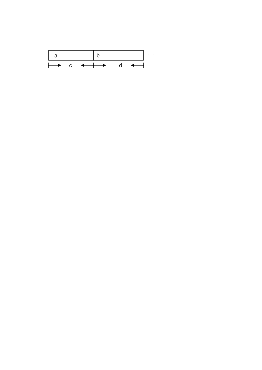
In the previous section, CB designs have been studied under the assumption that the EIC $\mbox{\boldmath{$G$}}_{\rm eff}$ is perfectly estimated at CR-Tx. In this section, we will study the effect of imperfect estimation of $\mbox{\boldmath{$G$}}_{\rm eff}$ due to finite sample size $N$ on the performance of the proposed CB scheme. First, consider the following two-phase protocol for CRs to support the learning-based CB scheme as shown in Fig. 3, where each block transmission of the CR with duration $T$ is divided into two consecutive sub-blocks. During the first sub-block of duration $\tau$, the CR observes the PR transmissions and estimates $\mbox{\boldmath{$G$}}_{\rm eff}$; during the second sub-block of duration $T-\tau$, the CR transmits data with the CB design based on the estimated $\mbox{\boldmath{$G$}}_{\rm eff}$ (following the same procedure as in Section IV, but with the estimated $\mbox{\boldmath{$G$}}_{\rm eff}$ instead of its true value). Note that $T$ needs to be chosen such that, on the one hand, to be sufficiently small compared with the channel coherence time in order to maintain constant channels during each transmission block, and on the other hand, to be as large as possible compared with the inverse of the channel bandwidth in order to make $T$ constitute a large number of symbols to reduce the overhead of channel learning. In this paper, we assume that $T$ is preselected as a fixed value. For a given $T$, intuitively, a larger value of $\tau$ is desirable from the perspective of estimating $\mbox{\boldmath{$G$}}_{\rm eff}$, while a smaller $\tau$ is favorable in terms of the effective CR link throughput that is proportional to $(T-\tau)/T$. Therefore, there exists a general learning-throughput tradeoff for the proposed CB scheme,⁵⁵ 5 Note that the learning-throughput tradeoff includes the sensing-throughput tradeoff studied in [17] as a special case since CR channel sensing to detect PR’s on/off status [17] can be considered as a “hard” version of CR channel learning proposed in this paper. where different choices for the value $\tau$ lead to different tradeoffs between PR transmission protection and CR throughput maximization.

The rest of this section is organized as follows. We first present two practical algorithms for CRs to estimate $\mbox{\boldmath{$G$}}_{\rm eff}$ with a finite $N$ in Section V-A. Then, in Section V-B we analyze the so-called “effective leakage interference” at PR terminals for the proposed CB scheme due to estimation errors in $\mbox{\boldmath{$G$}}_{\rm eff}$. At last, in Section V-C we characterize the learning-throughput tradeoff for CRs by finding the optimal value of $\tau$ to maximize the CR link effective throughput, under the given $T$, $P_{\rm CR}$, and maximum tolerable leakage interference power level at PR_j’s.

References

- [1] J. Mitola, “Cognitive radio: an integrated agent architecture for software defined radio,” PhD Dissertation, KTH, Stockholm, Sweden, Dec. 2000.
- [2] A. Goldsmith, S. A. Jafar, I. Marić, and S. Srinivasa, “Breaking spectrum gridlock with cognitive radios: an information theoretic perspective,” Proc. IEEE, vol. 97, no. 5, pp. 894-914, May 2009.
- [3] N. Devroye, P. Mitran, and V. Tarokh, “Achievable rates in cognitive radio channels,” IEEE Trans. Inf. Theory, vol. 52, no. 5, pp. 1813-1827, May 2006.
- [4] A. Jovičić and P. Viswanath, “Cognitive radio: an information-theoretic perspective,” in Proc. IEEE Int. Symp. Inf. Theory (ISIT), Jul. 2006.
- [5] S. Haykin, “Cognitive radio: brain-empowered wireless communications,” IEEE J. Sel. Areas Commun., vol. 23, no. 2, pp. 201-220, Feb. 2005.
- [6] M. Gastpar, “On capacity under receive and spatial spectrum-sharing constraints,” IEEE Trans. Inf. Theory, vol. 53, no. 2, pp. 471-487, Feb. 2007.
- [7] A. Ghasemi and E. S. Sousa, “Fundamental limits of spectrum-sharing in fading environments,” IEEE Trans. Wireless Commun., vol. 6, no. 2, pp. 649-658, Feb. 2007.
- [8] L. Musavian and S. Aissa, “Capacity and power allocation for spectrum-sharing communications in fading channels,” IEEE Trans. Wireless Commun., vol. 8, no. 1, pp. 148-156, Jan. 2009.
- [9] X. Kang, Y. C. Liang, A. Nallanathan, H. Garg, and R. Zhang, “Optimal power allocation for fading channels in cognitive radio networks: ergodic capacity and outage capacity,” IEEE Trans. Wireless Commun., vol. 8, no. 2, pp. 940-950, Feb. 2009.
- [10] R. Zhang, “On peak versus average interference power constraints for protecting primary users in cognitive radio networks,” IEEE Trans. Wireless Commun., vol. 8, no. 4, pp. 2112-2120, Apr. 2009.
- [11] Y. Chen, G. Yu, Z. Zhang, H. H. Chen, and P. Qiu, “On cognitive radio networks with opportunistic power control strategies in fading channels,” IEEE. Trans. Wireless Commun., vol. 7, no. 7, pp. 2752-2761, Jul. 2008.
- [12] R. Zhang, “Optimal power control over fading cognitive radio channels by exploiting primary user CSI,” in Proc. IEEE Global Commun. Conf. (Globecom), Dec. 2008.
- [13] R. Zhang, S. Cui, and Y.-C. Liang, “On ergodic sum capacity of fading cognitive multiple-access and broadcast channels,” to appear in IEEE Trans. Inf. Theory. Available [Online] at arXiv:0806.4468.
- [14] R. Zhang and Y.-C. Liang, “Exploiting multi-antennas for opportunistic spectrum sharing in cognitive radio networks,” IEEE J. Sel. Topics Sig. Process., vol. 2, no. 1, pp. 88-102, Feb. 2008.
- [15] A. Paulraj, R. Nabar, and D. Gore, Introduction to Space-Time Wireless Communications, Cambridge University Press, 2003.
- [16] Q. H. Spencer, A. L. Swindlehurst, and M. Haardt, “Zero-forcing methods for downlink spatial multiplexing in multiuser MIMO channels,” IEEE Trans. Sig. Process., vol. 52, no. 2, pp. 461-471, Feb. 2004.
- [17] Y.-C. Liang, Y. Zeng, E. C. Y. Peh, and A. T. Hoang, “Sensing-throughput tradeoff for cognitive radio networks,” IEEE Trans. Wireless Commun., vol. 7, no. 4, pp. 1326-1337, Apr. 2008.
- [18] T. J. Lim, R. Zhang, Y.-C. Liang, and Y. Zeng, “GLRT-based spectrum sensing for cognitive radio,” in Proc. IEEE Global Commun. Conf. (Globecom), Dec. 2008.
- [19] M. Wax and T. Kailath, “Detection of signals by information theoretic criteria,” IEEE Trans. Acoust., Speech, Sig. Process., vol. 33, no. 2, pp. 387-392, Apr. 1985.
- [20] F. Gao, Y. Zeng, A. Nallanathan, and T.-S. Ng, “Robust subspace blind channel estimation for cyclic prefixed MIMO ODFM systems: algorithm, identifiability and performance analysis,” IEEE J. Sel. Areas Commun., vol. 26, no. 2, pp. 378-388, Feb. 2008.
- [21] R. A. Horn and C. R. Johnson, Matrix Analysis, Cambridge University Press, 1985.
- [22] T. Cover and J. Thomas, Elements of Information Theory, New York: Wiley, 1991.
- [23] S. Boyd and L. Vandenberghe, Convex optimization, Cambridge University Press, 2004.