Alignment of Galaxies and Clusters
Abstract
We investigated the influence of environment on cluster galaxies by examining the alignment of the brightest cluster galaxy (BCG) position angle with respect to the host cluster X-ray position angle. The cluster position angles were measured using high spatial resolution X-ray data taken from the Chandra ACIS archive, that significantly improved the determination of the cluster shape compared to the conventional method of using optical images. Meanwhile, those of the BCGs were measured using homogeneous dataset composed of high spatial resolution optical images taken with Suprime-Cam mounted on Subaru 8m telescope.
We found a strong indication of an alignment between the cluster X-ray emission and optical light from BCGs, while we see no clear direct correlation between the degree of ellipticity of X-ray and optical BCG morphologies, despite the apparent alignment of two elliptical structures. We have also investigated possible dependence of the position angle alignment on the X-ray morphology of the clusters, and no clear trends are found. The fact that no trends are evident regarding frequency or degree of the alignment with respect to X-ray morphology may be consistent with an interpretation as a lack of dependence on the dynamical status of clusters.
Keywords:
Galaxies: clusters: general – X-rays: galaxies: clusters – Galaxies: evolution1 Introduction
It is well established that the major axes of galaxy clusters tend to point toward their nearest neighbour (e.g. Binggeli, 1982; Flin, 1987; Rhee & Katgert, 1987; Plionis, 1994; West et al., 1995; Plionis & Basilakos, 2002; Chambers et al., 2000; Chambers et al., 2002, Hashimoto et al. 2007a).
Another alignment effect is that between the orientation of the brightest cluster galaxy (BCG), or cD galaxy, and that of their parent cluster (Sastry, 1968; Dressler, 1978; Carter & Metcalfe, 1980; Binggeli, 1982; Struble, 1990; Plionis et al., 2003, e.g.). Similar alignment is also reported for poor groups of galaxies (Fuller et al., 1999). Numerical work (West et al., 1991; van Haarlem & van de Weygaert, 1993; West, 1994; Onuora & Thomas, 2000; Splinter et al., 1997; Faltenbacher et al., 2005, e.g.) show that substructure-cluster alignments can occur naturally in hierarchical clustering models of structure formation such as the cold dark matter model.
Unfortunately, all of these previous galaxy-cluster alignment studies are using optically-determined cluster position angles, most of them are based on the Palomar Observatory Sky Survey (POSS). Despite the importance of these optical investigations, individual galaxies may not be the best tracers of the shape of a cluster. Problems can arise from foreground/background contamination, as well as the fact that galaxies contribute discreteness noise. However, it is believed that the X-ray emitting gas within a cluster traces its gravitational potential (Sarazin, 1986). X-ray morphology may then be one of the best observable phenomenon for determining the cluster shape and orientation. Indeed, there are several X-ray studies for cluster vs. neighbour-cluster alignment (e.g. Ulmer, McMillan & Kowalski, 1989; Chambers, Melott & Miller, 2000; Chambers, Melott & Miller, 2002, Hashimoto et al. 2007a), but there are few galaxy-cluster alignment studies using X-ray morphology, except for Porter, Schneider & Hoessel (1991) and Rhee & Latour (1991), where they investigated the BCG-cluster alignment using low spatial resolution X-ray data, as well as traditional cluster shape parameter from apparent galaxy distribution, and reported a significant alignment. Unfortunately, previous X-ray studies are mostly based on data. These data are important, but the exposure depths are small and the spatial resolution is rather low compared to recently available X-ray data. The low spatial resolution may not significantly affect relatively robust measures such as position angle in a direct way, but it will critically hinder the accurate removal of contaminating point sources and the accurate determination of cluster center, and that may significantly affect the estimate of cluster X-ray morphology including the position angle. Hence, a new investigation using deeper X-ray data with much higher spatial resolution is needed.
Here we report a new investigation of galaxy alignment with respect to its parent cluster, using the cluster position angle and ellipticity determined by high spatial resolution X-ray data taken from the Chandra ACIS archive. Meanwhile, position angle and ellipticity of BCGs are determined from optical images taken with Subaru 8m telescope. This paper is organized as follows. In Sec. 2, we describe our main sample and X-ray measures, in Sec. 3, details of our optical data are described. Sec. 4 summarizes our results. Throughout the paper, we use = 70 km s-1 Mpc-1, =0.3, and =0.7, unless otherwise stated.
2 The X-ray Sample, X-ray Data Preparation, and X-ray measures
Here we briefly summarize our main X-ray sample, X-ray data preparation, and X-ray measures. More detailed descriptions can be found in Hashimoto et al. (2007b).
Almost all clusters are selected from flux-limited X-ray surveys, and X-ray data are taken from the Chandra ACIS archive. A lower limit of z = 0.05 or 0.1 is placed on the redshift to ensure that a cluster is observed with sufficient field-of-view with ACIS-I or ACIS-S, respectively. The majority of our sample comes from the Brightest Cluster Sample (Ebeling et al., 1998, BCS;) and the Extended Brightest Cluster Sample (Ebeling et al., 2000, EBCS;). When combined with EBCS, the BCS clusters represent one of the largest and most complete X-ray selected cluster samples, which is currently the most frequently observed by . To extend our sample to higher redshifts, additional high-z clusters are selected from various deep surveys; 10 of these clusters are selected from the Deep Cluster Survey (Rosati et al., 1998, RDCS;), 10 from the Extended Medium Sensitivity Survey (Gioia et al., 1990; Henry et al., 1992, EMSS;), 14 from the 160 Square Degrees Survey (Vikhlinin et al., 1998), 2 from the Wide Angle Pointed Survey (Perlman et al., 2002, WARPS;), and 1 from the North Ecliptic Pole survey (Henry et al., 2006, NEP;), RXJ1054 was discovered by Hasinger et al. (1998), RXJ1347 was discovered in the All Sky Survey (Schindler et al., 1995), and 3C295 has been mapped with Henry & Henriksen (1986).
The resulting sample contains 120 clusters. At the final stage of our data processing, to employ our full analysis, we further applied a selection based on the total counts of cluster emission, eliminating clusters with very low signal-to-noise ratio. Clusters whose center is too close to the edge of the ACISCCD are also removed. The resulting final sample contains 101 clusters with redshifts between 0.05 - 1.26 (median z = 0.226), and bolometric luminosity between 1.0 1044 – 1.2 1046 erg s-1 (median 8.56 1044 erg s-1). We reprocessed the level=1 event file retrieved from the archive. The data were filtered to include only the standard event grades 0,2,3,4,6 and status 0, then multiple pointings were merged, if any. We eliminated time intervals of high background count rate by performing a 3 clipping of the background level. We corrected the images for exposure variations across the field of view, detector response and telescope vignetting.
We detected point sources using the CIAO routine celldetect with a signal-to-noise threshold for source detection of three. We removed point sources, except for those at the center of the cluster which was mostly the peak of the surface brightness distribution rather than a real point source. The images were then smoothed with Gaussian =5”. We decided to use isophotal contours to characterize an object region, instead of a conventional circular aperture, because we did not want to introduce any bias in the shape of an object. To define constant metric scale to all clusters, we adjusted an extracting threshold in such a way that the square root of the detected object area times a constant was 0.5 Mpc, i.e. const = 0.5 Mpc. We chose const =1.5, because the isophotal limit of a detected object was best represented by this value.
The morphology of cluster X-ray emission is then characterized objectively by the position angle, as well as the ellipticity and the asymmetry. The position angle is defined by the orientation of the major axis measured east from north. Ellipticity is simply defined by the ratio of semi-major (A) and semi-minor axis (B) lengths as:
| (1) |
where
A and B are defined by the
maximum and minimum spatial rms of the
object profile along any direction and computed from the
centered-second moments by the formula:
| (2) | |||||
| (3) |
The asymmetry is measured by first rotating a cluster image by 180 degrees around the object center, then subtracting the rotated image from the original unrotated one. The residual signals above zero are summed and then normalized. Please see Hashimoto et al. 2007b for more detailed definitions of morphological measures.
3 Optical data
To determine the position angle and the ellipticity of BCGs, we used optical broad band images taken with Supreme-Cam (Miyazaki et al., 1998) on the Subaru telescope. The data were retrieved from Subaru-Mitaka-Okayama-Kiso Archive (SMOKA). Reduction software developed by Yagi et al. (2002) was used for flat-fielding, instrumental distortion correction, differential refraction, sky subtraction, and stacking. The camera covers a 34’ 27’ field of view with a pixel scale of 0202. The photometry is calibrated to Vega system using Landolt standards (Landolt, 1992). We refine the original astrometry written as WCS keyword in the distributed archival data using using USNO-A2 catalog with positional uncertainties less than 0.2 arcsec. The data were taken under various seeing conditions, and we used only images with less than 12 seeing. The optical data retrieved from SMOKA contains 30 clusters with redshifts between 0.08 - 0.9,
Some clusters have observed through many wavebands, and that allowed us to investigate the possible variations of our measures caused by waveband shifts. We have decided to rely primarily on the R band images for this alignment study, because we found that the effect of waveband shift is negligible.
The position angle and ellipticity of BCGs are measured exactly the same way as the X-ray cluster emission, namely, the position angle is defined by the orientation of the major axis measured east from north, and the ellipticity is defined by the ratio of semi-major and semi-minor axis. Please see Hashimoto et al. 2007b (Hashimoto et al., 1998, see also) for further details. As a precaution, we investigate the effect of superposed small galaxies sometimes lying on top of the extended structure of some BCGs, and we found that these superposed small galaxies have little effect on our robust measures such as, position angle and ellipticity.
4 Results
4.1 Systematics
One of the haunting, yet unfortunately often lightly treated, problem of any study comparing complex morphological characteristics of astronomical objects is the possible systematics introduced by various data quality, exposure times and object redshifts. Depending on the sensitivity of measures of characteristics, some susceptible measures may be seriously affected by these systematics, producing the misleading results.
Unfortunately, investigating the systematics on the complex characteristics is not an easy task. To investigate the systematic effect of, for example, various exposure times, one of the standard approaches is to simulate an image with a given exposure time by using an exposure-time-scaled and noise-added model image. Unfortunately, we need to approximate the various characteristics of a model to the complicated characteristics of a real object, (and those characteristics are often what we want to investigate) and this is an almost impossible task.
Meanwhile, if we use the real data, instead of the model, we will not have this problem. We can simulate lower signal-to-noise data caused by a shorter integration time by scaling the real data by the exposure time, and adding Poisson noise taking each pixel value as the mean for a Poisson distribution. However, this simple rescaling and adding-noise process will produce an image containing an excessive amount of Poisson noise for a given exposure time, thus lead us to underestimate the data quality. This inaccurate estimate of noise is caused by the intrinsic noise already presented in the initial real data. The intrinsic noise is difficult to be removed without sacrificing the fine spatial details of the object.
Similarly, to investigate the effect of dimming and smaller angular size caused by higher redshifts, in addition to the rest waveband shift effect, simple rescaling and rebinning of the real data will not work, because these manipulations will again produce the incorrect amount of noise.
Further difficulty associated with simulation using the real data comes from the fact that exposure and redshift effects are often coupled, because, in the real observation, low redshift objects are usually observed with shorter exposures than high redshift objects. This coupling further poses a serious problem, because simple standard method of simulating an observation with ‘decreased’ exposure time will force high redshift data to get degraded, which greatly reduces signal-to-noise ratio of already low quality high redshift data.
To circumvent all of these challenging problems, we developed a very useful simulating technique employing a series of ‘adaptive scalings’ accompanied by a noise adding process applied to the real images. This technique allows us to simulated an image of desired fiducial exposure time and redshift with correct signal-to-noise ratio without using a tricky artificial model image, thus we can easily investigate the effect of various image quality and/or easily change the real data to common fiducial exposure and redshift for easy comparison. Moreover, the technique can provide us with a powerful tool for conducting evolutionary studies, enabling us to compare the local objects to the high redshift objects without degrading photon-expensive high redshift data of low signal-to-noise ratio at all. This method is originally developed for the comparison of X-ray image data, but can be used for almost all kind of imaging data, including optical and NIR images.
Here we briefly describe the method. Please see Hashimoto et al. 2007b for further details. To simulate data with integration t=t1, an original unsmoothed image (including the background) taken with original integration time t0 was at first rescaled by a factor R0/(1-R0), instead of simple R0, where R0=t1/t0, t0t1. That is, an intermediate scaled image I1 was created from the original unsmoothed image I0 by:
| (4) |
Poisson noise was then added to this rescaled image by taking each pixel value as the mean for a Poisson distribution and then randomly selecting a new pixel value from that distribution. This image was then rescaled again by a factor (1-R0) to produce an image whose signal is scaled by R0 relative to the original image, but its noise is approximately scaled by , assuming that the intrinsic noise initially present in the real data is Poissonian.
Similarly, to simulate the dimming effect by the redshift, an intermediate scaled image I1 is created from the background subtracted image I0 by a pixel-to-pixel manipulation:
| (5) | |||||
| (6) |
where z0 and z1 are the original redshift and the new redshift of the object, respectively, and B is the background.
Finally, to simulate the angular-size change due to the redshift difference between z0 and z1, the original image will be rebinned by a factor R2, then intermediate scaled image will be created by rescaling the rebinned image by a factor 1/(R-1), before the addition of the Poisson noise. For the simulation with ‘increased’ exposure time, this factor can be changed to R3/(R-R3) where R3 = t2/t0, t2t0, where t2 is the increased exposure time, and t0 is the original integration time, and (R -R3) 0. The maximum length of integration time we can ‘increase’ (t2max) is naturally limited by the original exposure time and how much we increase the redshift for the redshift-effect part, and determined by the relationship,
| (7) |
which is equivalent to the case when no Poisson noise is added after the rebinning. Thus,
| (8) |
This t2max can be also used as a rough estimate of the effective image depth. The t2max provides an estimate of the image depth much more effectively than the conventional simple exposure time because t2max is related to a quantity that is affected both by exposure time and redshift, and thus enabling us to quantitatively compare exposure times of observations involving targets at different redshifts (e.g. 100 ksec at z=0.1 and 100 ksec at z=0.9).
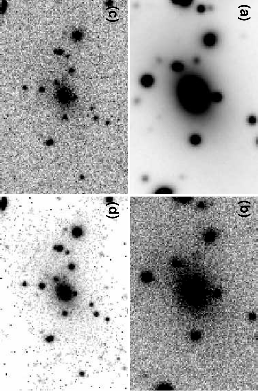

Although we suspected that our ellipticity and position angle were quite robust, as a precaution we investigated the possible systematics on these measures introduced by various exposure times and redshifts, using our scaling technique described above.
In Fig. 1, we demonstrate our technique of simulating desired exposure time and redshift using the real optical image of the BCG at the cluster center taken with Subaru Suprime-Cam. Original and modified exposure time and redshift of an example cluster (Abell 2219) are shown with north up and east left, where (a) original image: exptime(t)=240s, and redshift(z)=0.228, (b) simulated shorter exposure image with t=10s, (c) simulated high-z image with z=0.9, t=240s, and (d) simulated prolonged exposure at high-z with t=1092s, z=0.9.
Similarly, in Fig. 2, we use the real X-ray images of Abell 2219 from Chandra ACIS, and simulated various exposures and redshifts, where (a) original image with t=41ks, z=0.228, (b) simulated shorter exposure: t=10ks (z=0.228), (c) simulated High-z image: z=0.9 (t=41ks), and (d) prolonged exposure at High-z: t=188ks, z=0.9.
Using this technique, we simulated datasets with various exposure times and redshifts, and measured our cluster parameters. We found that our X-ray and optical position angles are robust against various exposure times and redshifts. Similarly, we found that other morphological measures such as, the ellipticity and asymmetry are quite robust, as well.
4.2 Analyses
| Cluster | z | PA_X | PA_BCG | PAa | Elli_X | Elli_BCG |
|---|---|---|---|---|---|---|
| (redshift) | (degree) | (degree) | (degree) | |||
| a2034 | 0.110 | 206.9 | 22.24 | 4.65 | 0.15 | 0.50 |
| a2069 | 0.114 | 327.7 | 331.8 | 4.18 | 0.46 | 0.66 |
| a750 | 0.163 | 249.0 | 249.6 | 0.66 | 0.14 | 0.31 |
| rxj1720 | 0.164 | 355.3 | 32.08 | 36.7 | 0.15 | 0.34 |
| a520 | 0.203 | 192.4 | 228.6 | 36.2 | 0.26 | 0.49 |
| a963 | 0.206 | 175.9 | 347.0 | 8.85 | 0.15 | 0.42 |
| a2261 | 0.224 | 225.8 | 14.48 | 31.3 | 0.14 | 0.13 |
| a2219 | 0.228 | 309.5 | -79.5 | 29.0 | 0.38 | 0.42 |
| a2390 | 0.233 | 298.6 | -57.6 | 3.76 | 0.30 | 0.32 |
| rxj2129 | 0.235 | 246.0 | 65.28 | 0.71 | 0.21 | 0.54 |
| a2631 | 0.278 | 258.2 | 84.27 | 6.07 | 0.29 | 0.41 |
| a1758 | 0.280 | 308.7 | 85.53 | 43.2 | 0.47 | 0.21 |
| a2552 | 0.299 | 201.7 | 216.4 | 14.7 | 0.18 | 0.45 |
| a1722 | 0.327 | 204.4 | 357.7 | 26.6 | 0.27 | 0.14 |
| zwcl3959 | 0.351 | 333.4 | 346.7 | 13.3 | 0.21 | 0.36 |
| a370 | 0.357 | 187.2 | 86.96 | 79.7 | 0.37 | 0.11 |
| rxj1532 | 0.361 | 227.7 | 78.24 | 30.5 | 0.18 | 0.37 |
| zwcl1953 | 0.373 | 351.2 | 306.3 | 44.8 | 0.24 | 0.51 |
| zwcl2661 | 0.382 | 159.5 | 206.9 | 47.3 | 0.12 | 0.43 |
| zwcl0024 | 0.390 | 5.200 | 246.6 | 61.4 | 0.03 | 0.48 |
| rxj2228 | 0.412 | 263.7 | 56.27 | 27.4 | 0.21 | 0.54 |
| rxj1347 | 0.451 | 359.2 | 343.8 | 15.3 | 0.20 | 0.13 |
| ms0451 | 0.540 | 279.9 | 344.9 | 65.0 | 0.26 | 0.04 |
| cl0016 | 0.541 | 228.7 | 244.6 | 15.9 | 0.19 | 0.31 |
| ms2053 | 0.583 | 304.8 | 336.8 | 32.0 | 0.25 | 0.16 |
| rxj1350 | 0.810 | 334.2 | 308.9 | 25.2 | 0.20 | 0.47 |
| rxj1716 | 0.813 | 236.2 | 255.1 | 18.9 | 0.17 | 0.52 |
| ms1054 | 0.830 | 266.1 | 35.96 | 50.1 | 0.40 | 0.51 |
| rxj0152 | 0.835 | 221.6 | 231.0 | 9.46 | 0.58 | 0.29 |
| wga1226 | 0.890 | 284.5 | 264.6 | 19.8 | 0.09 | 0.15 |
a: PA is an acute angle of PA_BCG-PA_X

Table 1 shows a summary of our optical cluster sample, where PA is an acute relative angle between the position angle of X-ray (PA_X) and BCG (PA_BCG), namely, the relative position angle differences greater than 90 degree are ‘folded’ and changed to be acute ranging between 0 and 90 degree. Despite the robust nature of our measures, we modify, as a precaution, all of the X-ray and optical observations to be equivalent to z=0.9 and t=t2max to eliminate any possible small systematics, but otherwise to maximize the image quality.
In Fig. 3, the ellipticity of cluster X-ray morphology is plotted against the ellipticity of optical morphology of BCGs. Interestingly, in spite of expected alignment of two elliptical structures, there are a large scatter and we found no strong correlation in the relationship between the two ellipticities.


Fig. 4 shows the acute relative position angle difference between cluster X-ray morphology and BCG morphology plotted against the ellipticity of BCGs (top panel) and the ellipticity of cluster X-ray morphology (bottom panel). Fig. 4 shows that the position angle difference tends to be smaller than 45 degree, implying that BCGs tend to elongated in the same direction of the X-ray distribution of their host clusters, particularly for clusters exhibiting relatively high ellipticity in their optical BCG morphology and/or in their cluster X-ray morphology. Meanwhile, for clusters with very low BCG or X-ray ellipticity (ellipticity 0.1) position angle are generally poorly determined, and thus position angle difference can be inaccurate.
Fig. 5 shows the frequency distribution of the position angle difference. There is a strong tendency that we have more clusters with an angle difference less than 45 degrees, consistent with the observation made in Fig. 4.
To test this trend more rigorously, we first employed the Kolmogorov-Smirnov (K-S) test. The null hypothesis here is that our sample can be drawn from a parent population of random position angle differences. However, the K-S test detects the deviation from the parent population (here the population of random position angle differences), thus it may loose some sensitivity for testing the cluster alignment, where it is likely that position angle difference is systematically lower than the random sample. To increase the sensitivity to an alignment signal, as a second test we employed the Wilcoxon-Mann-Whitney rank-sum test. The null hypothesis of this test is that the position angle difference is not systematically smaller or larger than the random sample. Therefore the test is insensitive to an excess of angles around the mean (i.e. 45 deg). When applied to our sample, both K-S and rank-sum tests show, not surprisingly the strong alignment signals, and we find that the null hypothesis can be rejected with 99.93% and 99.99% confidence, respectively, thus confirming that BCGs are significantly aligned to the X-ray emissions of the host clusters. We have also investigated the alignment of other luminous non-BCG galaxies to the X-ray emissions and we found no significant alignment. The results are summarized in table 2, where LG2 is the second brightest galaxy, LG3 is the third brightest galaxy, and LGn is the n-th brightest galaxy within a projected distance of 1 Mpc from the X-ray center.
| Statistics | BCG | LG2 | LG3 | LG4 | LG5 |
|---|---|---|---|---|---|
| K-S | 99.93 | 81.67 | 49.93 | 4.22 | 8.99 |
| Rank Sum | 99.99 | 83.06 | 57.09 | 54.51 | 63.33 |

In Fig. 6, we investigated possible dependence of the position angle alignment on the X-ray morphology of the clusters. In Fig. 6, the cluster X-ray asymmetry is plotted against cluster X-ray ellipticity. Large solid circles are clusters showing strong alignment between the cluster and BCG with position angle difference less than 20 degree, while solid triangles are clusters showing the alignment, but with position angle difference between 20 and 45 degree. Crosses represent clusters with no sign of the alignment, and small dots are clusters in our main X-ray sample without optical Subaru data. No clear trends are evident regarding frequency or degree of the alignment with respect to X-ray morphology.
We have also attempted to investigate possible dependence of the alignment on cluster redshifts. We found that for clusters less than z=0.35, both K-S and rank-sum tests show that the null hypothesis can be rejected with 99.92% and 99.99% confidence, respectively, while for clusters greater than or equal to z=0.35, alignment signals are somewhat weaker that the null hypothesis can be rejected with 93.88% and 83.69% confidence, respectively for K-S and rank-sum tests. Similarly, we have investigated the dependence of the alignment on the cluster X-ray bolometric luminosity (Lbol), and we did not find any significant trend: for clusters with Lbol greater than or equal to 2 1045 erg/s, the null hypothesis can be rejected with 93.45% and 96.42% confidence, while for clusters with Lbol smaller than 2 1045 erg/s, the null hypothesis can be rejected with 99.78% and 99.90% confidence, respectively for K-S and rank-sum tests.
5 Summary
We investigated the influence of environment on cluster galaxies by examining the alignment of the BCG position angle with respect to the host cluster X-ray position angle. The cluster position angles were measured using high spatial resolution X-ray data taken from the Chandra ACIS archive, that significantly improved the determination of the cluster shape compared to the conventional method of using optical images. Meanwhile, those of the BCGs were measured using high spatial resolution optical images taken with Suprime-Cam mounted on Subaru 8m telescope.
We found a strong indication of an alignment between the cluster X-ray emission and optical light from BCGs, while we see no clear direct correlation between the ellipticity of X-ray morphology and optical BCG morphology despite of the apparent alignment of two elliptical structures. In the hierarchical structure formation models, the alignment effect could be produced by clustering models of structure formation such as the cold dark matter model (Salvador-Sole & Solanes, 1993; West, 1994; Usami & Fujimoto, 1997; Onuora & Thomas, 2000; Faltenbacher et al., 2002; Faltenbacher et al., 2005, e.g.). The existence of the alignment effects is also consistent with a cosmic structure formation model such as the hot dark matter model (Zeldovich, 1970, e.g.), where clusters and galaxies form by fragmentation in already flattened sheet- and filament-like structures.
We have also investigated possible dependence of the position angle alignment on the X-ray morphology of the clusters, and no clear trends are found. If the X-ray morphology of clusters reflects dynamical status of clusters (Hashimoto et al., 2004, e.g.), the fact that no trends are evident regarding frequency or degree of the alignment with respect to X-ray morphology may be consistent with an interpretation as a lack of dependence of alignment on the dynamical status of clusters. Primordial galaxy alignments in clusters can be damped by various mechanisms such as the exchange of angular momentum in galaxy encounters, violent relaxation, and secondary infall (Quinn & Binney, 1992; Coutts, 1996, e.g.) over a Hubble time. Thus, in highly relaxed clusters, we might naively expect to observe weaker primordial galaxy alignment, because there has been sufficient time to mix the phases. The fact that we do not see any significant alignment trend with respect to the X-ray morphology may provide an important constrain on these damping scenarios.
Acknowledgments
This work is based in part on data collected at Subaru Telescope and obtained from the SMOKA, which is operated by the Astronomy Data Center, National Astronomical Observatory of Japan. We thank our referee, Dr. Michael West for his comments, which improved the manuscript. YH thanks Hiromi Hashimoto for the help retrieving the data from SMOKA.
References
- Binggeli (1982) Binggeli B., 1982, A&A, 107, 338
- Carter & Metcalfe (1980) Carter D., Metcalfe N., 1980, MNRAS, 191, 325
- Chambers et al. (2000) Chambers S., Melott A., Miller C., 2000, ApJ, 544, 104
- Chambers et al. (2002) Chambers S., Melott A., Miller C., 2002, ApJ, 565, 849
- Coutts (1996) Coutts A., 1996, Monthly Notices of the Royal Astronomical Society, 278, 87
- Dressler (1978) Dressler A., 1978, ApJ, 226, 55
- Ebeling et al. (2000) Ebeling H., Edge A., Allen S., Crawford C., Fabian A., Huchra J., 2000, MNRAS, 318, 333
- Ebeling et al. (1998) Ebeling H., Edge A., Böhringer H., Allen S., Crawford C., Fabian A., Voges W., Huchra J., 1998, MNRAS, 301, 881
- Faltenbacher et al. (2005) Faltenbacher A., Allgood B., Gottlober S., Yepes G., Hoffman Y., 2005, MNRAS, 362, 1099
- Faltenbacher et al. (2002) Faltenbacher A., Gottlober S., Kerscher M., Muller V., 2002, A&A, 395, 1
- Flin (1987) Flin P., 1987, MNRAS, 228, 941
- Fuller et al. (1999) Fuller T., West M., Bridges T., 1999, ApJ, 519, 22
- Gioia et al. (1990) Gioia I., Maccacaro T., Schild R., Wolter A., Stocke J., Morris S., Henry J., 1990, ApJS, 72, 567
- Hashimoto et al. (2004) Hashimoto Y., Barcons X., Böhringer H., Fabian A., Hasinger G., Mainieri V., Brunner H., 2004, A&A, 417, 819
- Hashimoto et al. (007b) Hashimoto Y., Boehringer H., Henry J., Hasinger G., Szokoly G., 2007b, A&A, 467, 485
- Hashimoto et al. (007a) Hashimoto Y., Henry J., Bohringer H., 2007a, MNRAS, 380, 835
- Hashimoto et al. (1998) Hashimoto Y., Oemler Jr A., Lin H., Tucker D., 1998, ApJ, 499, 589
- Hasinger et al. (1998) Hasinger G., Giacconi R., Gunn J., Lehmann I., Schmidt M., Schneider D., Truemper J., Wambsganss J., Woods D., Zamorani G., 1998, A&A, 340, L27
- Henry et al. (1992) Henry J., Gioia I., Maccacaro T., Morris S., Stocke J., Wolter A., 1992, ApJ, 386, 408
- Henry & Henriksen (1986) Henry J., Henriksen M., 1986, ApJ, 301, 689
- Henry et al. (2006) Henry J., Mullis C., Voges W., Bohringer H., Briel U., Gioia I., Huchra J., 2006, ApJS, 162, 304
- Landolt (1992) Landolt A., 1992, AJ, 104, 340
- Miyazaki et al. (1998) Miyazaki S., Sekiguchi M., Imi K., Okada N., Nakata F., Komiyama Y., 1998, Proc. SPIE, 3355, 363
- Onuora & Thomas (2000) Onuora L., Thomas P., 2000, MNRAS, 319, 614
- Perlman et al. (2002) Perlman E., Horner D., Jones L., Scharf C., Ebeling H., Wegner G., Malkan M., 2002, ApJS, 140, 265
- Plionis (1994) Plionis M., 1994, ApJS, 95, 401
- Plionis & Basilakos (2002) Plionis M., Basilakos S., 2002, MNRAS, 329, L47
- Plionis et al. (2003) Plionis M., Benoist C., Maurogordato S., Ferrari C., Basilakos S., 2003, ApJ, 594, 144
- Porter et al. (1991) Porter A., Schneider D., Hoessel J., 1991, AJ, 101, 1561
- Quinn & Binney (1992) Quinn T., Binney J., 1992, Monthly Notices of the Royal Astronomical Society, 255, 729
- Rhee & Katgert (1987) Rhee G., Katgert P., 1987, A&A, 183, 217
- Rhee & Latour (1991) Rhee G., Latour H., 1991, A&A, 243, 38
- Rosati et al. (1998) Rosati P., Della Ceca R., Norman C., Giacconi R., 1998, ApJ, 492, L21
- Salvador-Sole & Solanes (1993) Salvador-Sole E., Solanes J., 1993, ApJ, 417, 427
- Sarazin (1986) Sarazin C., 1986, RvMP, 58, 1
- Sastry (1968) Sastry G., 1968, PASP, 80, 252
- Schindler et al. (1995) Schindler S., Guzzo L., Ebeling H., Boehringer H., Chincarini G., Collins C., de Grandi S., Neumann D., Briel U., Shaver P., et al., 1995, A&A, 299, L9
- Splinter et al. (1997) Splinter R., Melott A., Linn A., Buck C., Tinker J., 1997, ApJ, 479, 632
- Struble (1990) Struble M., 1990, AJ, 99, 743
- Ulmer et al. (1989) Ulmer M., McMillan S., Kowalski M., 1989, ApJ, 338, 711
- Usami & Fujimoto (1997) Usami M., Fujimoto M., 1997, ApJ, 487, 489
- van Haarlem & van de Weygaert (1993) van Haarlem M., van de Weygaert R., 1993, ApJ, 418, 544
- Vikhlinin et al. (1998) Vikhlinin A., McNamara B., Forman W., Jones C., Quintana H., Hornstrup A., 1998, ApJ, 502, 558
- West (1994) West M., 1994, MNRAS, 268, 79
- West et al. (1995) West M., Jones C., Forman W., 1995, ApJ, 451, L5
- West et al. (1991) West M., Villumsen J., Dekel A., 1991, ApJ, 369, 287
- Yagi et al. (2002) Yagi M., Kashikawa N., Sekiguchi M., Doi M., Yasuda N., Shimasaku K., Okamura S., 2002, AJ, 123, 66
- Zeldovich (1970) Zeldovich Y., 1970, A&A, 5, 168