Persistence, extinction and spatio-temporal synchronization of SIRS cellular automata models
Abstract
Spatially explicit models have been widely used in today’s mathematical ecology and epidemiology to study persistence and extinction of populations as well as their spatial patterns. Here we extend the earlier work–static dispersal between neighbouring individuals to mobility of individuals as well as multi-patches environment. As is commonly found, the basic reproductive ratio is maximized for the evolutionary stable strategy (ESS) on diseases’ persistence in mean-field theory. This has important implications, as it implies that for a wide range of parameters that infection rate will tend maximum. This is opposite with present results obtained in spatial explicit models that infection rate is limited by upper bound. We observe the emergence of trade-offs of extinction and persistence on the parameters of the infection period and infection rate and show the extinction time having a linear relationship with respect to system size. We further find that the higher mobility can pronouncedly promote the persistence of spread of epidemics, i.e., the phase transition occurs from extinction domain to persistence domain, and the spirals’ wavelength increases as the mobility increasing and ultimately, it will saturate at a certain value. Furthermore, for multi-patches case, we find that the lower coupling strength leads to anti-phase oscillation of infected fraction, while higher coupling strength corresponds to in-phase oscillation.
Keywords:
Epidemiology; Phase transitions; Emergence of trade-offs; In-phasepacs
87.23.Cc, 05.40.-a, 82.40.CkI Introduction
In recent years, there has been an increased awareness of the threats posed by newly emerging and high-profile infections disease, such as SARS, the H5N1 strain of avian influenza, HIV, Ebola, Whooping cough, Dengue fever and the spread of influenza. These diseases exhibit large scale spatial contagions and long-term spatial patterns [1, 2, 3, 4, 5, 6, 7, 8, 9].
At present, there is a great deal of interest in the role of spatial structure in both ecology and epidemics. All systems are to some degree spatially extended; however, the classical theory of the dynamics of epidemics ignores spatial effects with its assumption of homogeneous mixing. It is likely that local processes will play an important role in the majority of infectious diseases’ interactions particularly when an infection occurs through the direct contact of infected and susceptible individuals [10, 11]. As a consequence, there has been some attempt to take explicitly spatial structure into account when examining the spreading of parasites [12, 13, 1, 14, 15, 16, 17]. For example, recent models show that interactions between local populations may generate complex spatial patterns by dispersal [14, 15, 1, 2, 18]. In modern societies, individuals can easily travel over a wide range of spatial scales. The interconnections of areas and populations through various means of transport have important effects on the geographical spread of epidemics [2]. In particular, the spatial structure and the different levels of the diffusion and transport processes are responsible for the heterogeneity, that is an erratic outbreak patterns observed in the worldwide propagation and persistence of diseases [19, 1, 3, 20, 6], recently documented for synchronization and waves [3, 20, 18, 21, 2, 8], and large-scale spatial patterns (e.g. spiral waves [1, 15, 22] and Turing patterns [23, 24]) in measles, dengue fever, SARS, and influenza. In order to describe such a complex phenomenon and develop powerful numerical forecasting tools, different levels of description are possible, ranging from a simple global mean-field to detailed individual-based simulation (see Refs. [25, 12, 26, 27, 28, 29, 30] and references therein), cellular automata [31, 32, 33, 14, 15, 1, 22, 34], coupled map lattices [35], etc.
Dispersing individuals may react in a complex manner to local ecological and epidemiological situations [2, 5, 36, 37, 22], but rare long-distance dispersal events may be important in nature [38, 39, 4, 22]. The modeling methods that summarize dispersal in a diffusion coefficient in the classical theory–partial differential equations–cannot give insights into the importance of rare events [16]. For humans and other social animals in which hosts are distributed in heterogeneous patches on a large scale, there are two critical sides to transmit. The first is local transmission among individuals within patches or communities (cites, towns, and villages). The second is the transmission between patches. With this point of view, there is a clear conceptual link between ecological and epidemiological theory; a body of recent works have focused on the analogies of the spatial dynamics between infectious disease and ecological metapopulations [6, 5, 40, 41]. The twofold issues are to dissect how infection processes at the local scale determine spatio-temporal patterns of epidemics and understand how these patterns are affected by the spatial spread between neighborhoods or patches, for instance, the epidemic wavefronts observed in the spatio-temporal spread of the Black Death in Europe from 1347 to 1350 [42, 18] and West Nile virus [43].
Generally speaking, several generic questions can be asked when studying the dynamics of epidemic spreading. One is the explanation of the possible oscillations 11 1 The sustained oscillations include the coherence resonance phenomenon in the epidemic models [101, 102, 69, 68]. with respect to the temporal evolution of the densities of infection waves in homogeneous or heterogeneous realistic situation, as well as the spatial resonance problem. Another one concerns the study of the possibility that a disease spreading eventually arrives at a steady states and the time arrived [25, 44]. In addition, our model can also investigate what enables some species to persist while others become extinct. This question has shaped the history of research on population dynamics and remains a central issue for ecologists and epidemiologists [6].
Although the spatial structure has been developed for susceptible-infected-resistant (SIRS) models in previous studies, the modulation of such effects in combination with individuals’ mobility is also unknown. We aim to bridge this gap in this paper. Specifically, we aim to elucidate the phase space on the extinction and persistence and contrast them with the prediction obtained mean-field, as well as the effect of mobility on persistence criteria. We also examine how the spatial pattern depend on the mobility and coupling strength within multi-patches case.
II Model and methods
II.1 Cellular automata model
In a recent report, van Ballegooijen and Boerlijst (vBB) showed that there were three types of spatial pattern in a spatial susceptible-infected-resistant model for disease dynamics by using a grid-structured contact network, also called cellular automata model [1]. They were localized disease outbreaks with self-limiting in size, turbulent waves, and stable spiral waves respectively. Furthermore, they predicted that there existed a trade-off between the parameters of infection period and infection rate, which emerges from the evolutionary dynamics of the system on the stable spiral waves, and referred to this relationship as emergent trade-off. These results give a guide to understand the spatial features of epidemic such as wave speed and wavelength, as well as the persistence and extinction relationship depending on the parameters. To model the spatio-temporal phenomena, a feasible approach is the combination of grid-based models and movements of individuals. In this paper we take the framework proposed by vBB as a starting point in assessing the phase transitions between the persistence and extinction rather than emergence of the stable spiral waves.
We use a spatial susceptible-infected-resistant model. The population with individuals is categorized according to its infection status: susceptibility (S), infectious (I), or resistant (R) [45, 1, 3, 20]. Within a subpopulation, the dynamics for the local populations obey a basic reaction scheme conserving the number of population, which has been studied both in physics and mathematical epidemiology, namely the stochastic infection dynamics process identified by the following set of reactions [1]
| (1a) | |||
| (1b) | |||
| (1c) |
The first reaction (Eq. (1a)) reflects the fact that an infected host (I) can infect susceptible (S) neighbors with infection rate ; the second reaction (Eq. (2b)) indicates the acquisition of resistance that hosts are infectious for a fixed period , after which they become resistant (R); and the third reaction (Eq. (1c)) indicates the loss of resistance that after a fixed period , resistant hosts once again become susceptible. In the sense of individual/local-level model, infected hosts can infect adjacent susceptible hosts at infection rate . Here, the infection rate is not equal the probability of infection, see [1, 46, 5]. In the short-range case, the infectious neighborhood consists of two/eight direct nearest-neighbors (NN) in a 1D/2D square lattices. In addition, some recent investigations have included long-range processes in one- and two-dimensional lattice models, reporting quite different results on the occurrence of self-sustained oscillation, extinction and persistence [47, 48, 49, 50, 51, 52, 53, 54, 55], as well as increasing coupling between subpopulation (subcommunity) in spatially structured environment can lead to population outbreaks [56, 5, 2]. Thus, an understanding of the joint effect of short- and long-range interaction on the individuals (including the mobility called as the diffusion, hopping, or stirring, hereafter, we refer as mobility) is desirable from ecological and statistical physical point of view [57]. Of course, in present paper, we also further study the outbreak of disease inspired stochastic lattice epidemic model with a nearest-neighbor interaction.
For ease of comparison, we follow the vBB’s model by considering a regular network of sites, each of which contains one of a single susceptible individual (S), an infected individual (I) and resistant (R). The susceptibles are infected by contact with an infected host at a rate , and the transmission can only occur locally. Every time-step , cells’ state change according to the rules in earlier studies [1, 3], which are illustrated in the corresponding Eq. (1).
II.2 Rate equations
The deterministic rate (or mean-field) equations describe the temporal evolution of the stochastic lattice system, defined by the reactions (1), in a mean-field context, i.e. they neglect all spatial correlations. They may be seen as a deterministic description (for example emerging in the limit of large system sizes) of systems without spatial structure. The study of the rate equation is the ground on which the analysis of the epidemics spreading and outbreak. In particular, the properties of the rate equations are extremely useful for the epidemics persistence by estimated values for the classical expression of –the basic reproduction number. is defined as the number of secondary infections caused by a single infective during its infectiousness period in an entirely susceptible population [45, 42]. For the standard SIRS mean-field approximation, also referred in reaction (1), are as follows:
| (2a) | |||
| (2b) |
where and denote the number of susceptibles and infected, respectively. The number of recovered individual is obtained by conservation of the entire population, i.e., . The key quality describing the infection is the basic reproduction number . If and the initial relative number of susceptibles are greater than a critical value , an epidemic develops (). As the number of infected individuals increases, the number of susceptibles decreases, and thus the number of contacts of infected individuals with susceptibles decreases until , when the epidemic reaches its maximum and subsequently decays. This processes alternative again with the time going if . Fadeout is most likely to occur in the period immediately following a major epidemic (the so-called inter-epidemic trough). An important observation is that deterministic models cannot reproduce such effects: the ability of populations to recover from very low levels is a well-known weakness of many deterministic models [8, 58].
III Simulation and Results
To begin with, we revisit some of the findings by vBB [1]. Their results then serve as a reference point for illustrating the difference of our elaborated approach from their results. This is justified by the fact that vBB only provide the spatial pattern resulting from static dispersal among individuals within single patch, as well as emergence of trade-offs between spiral waves and turbulent waves. Our crucial measures are the phase transition between the global extinction and persistence of the epidemic, and the effect from the movements of individuals on it. In these simulations we set there is no migration among patches, i.e., coupling parameter , in which our simulations faithfully repeat the general findings by VBB [1] that three types of spatial patterns emerge (see Fig. 1) but find the differences when the mobility of individuals is turned on.
III.1 Phase transitions of persistence and extinction
In this subsection, we analyze the relationship of infection rate and infection periodic on phase transition between global persistence and extinction within single patch. In the final subsection, we will introduce the multipatches into the spatial structure model by the coupling strength between the two patches.
When the individuals are statical in the local site, then the infection only happens in the nearest neighbors, this form referred to as local interaction. Specially, we can study the dynamics of such spatially extended model in one- or two-dimensional space by defining appropriate microscopic rules. Equation (1) shows the explicit transition rates of cells’ state in space, where the susceptibles infected by infectious is isotropic. Grid size used in the simulations is cells and time-step equals to 0.01. Larger grid sizes do not change the evolutionary dynamics (see the computer code for the CA model at http://7y.nuc.edu.cn/jinzhen/English1.aspx).
The persistence phase space is that the epidemics will persist when the parameters lie in this domain. Here, we refer to -parameters space. Their values are determined by simulating cell lattices with ten independent runnings. Each lattice is initially set with random occupied by 100 infected individuals. For each obtained data, we fix the infection period , and chose an initial infection rate . Then, increased by small step (we use ) and 10 thousand time units are simulated with that infection rate value to determine the critical value of the phase transition. Here, we find that 10 thousand time units is a long-term run for persistence on this system. However, the typical waiting time until extinction occurs is generally very long when the system size is large. This suggests to consider the dependence of the waiting time on . Quantitatively, we discriminate between persistence and extinction by using the concept of extensively, adapted from statistical physics [60, 59]. If the epidemic is not extinct at that time, the pair parameters’ values are assumed to be within the persistence space. In the present model, we find that the epidemic will be persistence when parameter is between a minimal critical infection rate and a maximal critical infection rate . It is also worth noticing that the definitions of persistence and extinction in the presence of absorbing states are intimately related to the concept of long-term.
The threshold result for the deterministic model can be used to identify two domains in the space of essential parameters , namely and , where the model solutions behave in qualitatively different ways. We endeavor to describe the spatially stochastic model in a similar way, by identifying domains in the space of its essential parameters where model solutions behave in qualitatively different ways. We perform extensive computer simulations of the system (1) on the phase transition, which describes the persistence and extinction with respect to the -parameters space shown in Fig. 2 which also demonstrates that there exists a trade-off between infection period and infection rate. In order to compare the classic mean-field approximation of non-spatial theory and the spatial structure of individuals on the phase transition, we use the power laws to fit the simulation data. Moreover, previous studies show that the infection rate () and the virulence () also have a relation of power laws on the parameters of the infection rate and virulence [61, 62]. Yet, this relationship can be expressed generally with formula, as shown in Fig. 2, in which the red curve and blue curve are fitted by this function with 95% confidence intervals on the parameter estimates, respectively. As could be expected, there exist minimal and maximal critical values of the infection rate on the phase transition. The open circles () and faced circles () indicate the simulated results of the minimal critical infection rate and maximal critical infection rate , respectively. By comparison between fitted curves and simulations, one can see there is a nonlinear trade-off, is a monotonically decreasing function of and bounded by a positive constant. The dashed line in Fig. 2 show the prediction on the phase space from mean-field theory on . From the classical expression of , we know that the diseases will die out if . This has important implications, as it implies that for a wide range of space there are two parameter domains in the space. One is domain of extinction and the other is domain of persistence. This contrast with the result obtained in spatially explicit model where the parameter domain is divided into three: domains (I) disease free; domain (II) endemic (see Fig. 2). The numerical results clearly indicate (see Fig. 2, Inset) the validity of the prediction for the spatial thresholds to control invasion of parasites. In the - plot (Inset of Fig. 2), the dashed line and power laws () is straight line of slope shown on the graph. Then, the same where is plotted against . One can see that a nonzero (nonvanishing infection rate) is better straight line. In this case, the nonzero corresponds to the phase boundaries for large . The best-fit line on a - scale has a slope of -0.7065, indicating a linear dependence of on . An understanding of this scaling behavior is lacking.
(a) (b)
(b) (c)
(c)
The classical mean-field theory on the diseases spreading has shown that the number of number of secondary cases due to a single infected individual (referred is maximized in the model (2) and therefore maximum transmission is selected. Here, our results show that once the spatial structure is included the is no longer maximized and the transmission rate is limited (see the labeled a in Fig. 2). We note that this results are consistent with parasite evolution and extinction [62]. In addition, in the spatial explicit model, the diseases can survive for a lower infection rate than mean-field context. This is a low infection rate will tend to increase the local density of susceptible individual around infectious. Spatial structure within cluster of individual favors a lower infection rate. The other way round, with higher infection rate will tend to infect all the individuals in a cluster quickly. This in turn leads to relatively rapid local cluster extinction.
Moreover, we also find that, for the fixed infection period , the different moving spatial patterns emerge with infection rate increasing. Figure 1 shows the typical snapshots of the stable spatial patterns when the parameters are within domain of persistence II in Fig. 2, in which the results indicate that the threshold values is equal to and equal to for respectively. When the infection rate is low (but just above the critical value ), we find that the susceptible and infectious individual coexist, and self-organized spatial patterns with limited size of moving clusters. It means that localized disease outbreaks are self-limiting in size for this case (see Fig. 1(a)). With increasing infection rate , these structures grow in size and form pattern of moving turbulent/spirals (see Fig. 1(b) and (c)), and disappear for large enough (exceed the critical value ).

Bartlett observed in a series of papers [63, 64, 65] that measles in large cities had recurring outbreaks, while it went extinct in small communities until reintroduced from external sources. This means that the time to extinction is an increasing function of the community size. However, the analysis by Nasell showed that Bartlett’s approximation of the extinction time was unsatisfactory in an important part of parameter space [66, 67]. Our present system (1) is a simple individual-based stochastic SIRS model with diffusion processes [68, 69, 70, 71]. The goal of the analysis is to derive information about the quasi-stationary distribution and the time to extinction. Pursuing this goal leads to difficult mathematical problems. Exact solutions cannot be found. A possible way to proceed is therefore to work with approximations by simulation. Early efforts to derive approximations of the expected time to extinction were shown by Nasell to lead to large errors [66]. In the present paper, a approximation of the discrete state Markov chain (1) is introduced. It led to a truncated normal distribution as an approximation of the marginal distribution of infected individuals in quasi-stationarity [72, 73, 67]. The resulting approximation of the expected time to extinction was rather coarse by a linear relation, but turned out to be an accepted approximations for present analysis of extinction and persistence.
The dependence of the average time () to extinction on the system size of changes, , is shown in Fig. 3, which also demonstrates the dependence of on the size of the populations when the parameters are within domain of extinction. As seen, average extinction time increases linearly with system size (we test the system size from 10,000 to 90,000). More quantitatively, is approximately proportional to , which is fitted the simulation results by using linear function, and then obtain the relationship as are shown in Fig. 3. To ensure that the used averaging over just 100 independent runs yields good statistics, we present in Fig. 3 the each data of obtained 100 runnings for and (these parameters corresponding to extinction lower domain I in Fig. 2.). It should be noticed that previous phase transitions analysis is convincible because third time to extinction was used to estimate phase transitions of persistence and extinction. One can seen that 10 thousand time units are a long-term run for persistence on this system. Here, it is instructive to note that our results show that the persistence and extinction are independent on the population size. The opposite view have been obtain from the well-mixed systems in recently Ref. [74], in which they demonstrate a critical population size above which coexistence is likely.

III.2 Mobility promotes persistence on spatial epidemic model
In fact, the individual always exhibits motion in the space. How does individuals mobility, in addition to nonlinearity, affect the system’s behaviors (i.e., persistence and extinction, spatial pattern, invasion speed and so on)? The insight of this important issue can be gained from the cellular automata model. In particular, one can compare the results of present paper with the previous works [1]. Two models are commonly used to predict spatial spread of a disease. The first is the distributed-contacts model, often described by a contact distribution among stationary individuals. Distributed-contacts models are particularly appropriate for the study of plant disease [75, 76], but researchers are also using the closely related framework of contact networks to study disease transmission in human population [77, 78] or animal species. Notice that recently developing spatial moment closure methods are also based on this framework [79, 80]. The second is the distributed-infectives models, often described by the mobility of infected individuals. This approach relies on the assumptions that disease is transmitted through interactions between dispersing individuals, and that infected individuals move in uncorrelated random walks. Medlock and Kot developed a distributed-infectives framework that uses a flexible kernel-based approach similar to that employed in distributed-contact models [81]. They found that inappropriate application of either the distributed-contact or distributed infectives approaches can generate inaccurate projections of epidemic spread. Hence, here we consider a scenario that the transmission process involves components of both distributed-contacts and distributed infectives–diffusion of infected individuals. For instance the spread of rabies that foxes tend to be restricted to discrete home ranges. In Central Europe, the home range size is about 4 , but this may differ considerably between areas (range 2.5-16 ) [82, 22]. Based on previous subsection, now we investigate the individuals with a certain form of mobility. Namely, at rate all individuals can exchange their position with a nearest neighbor. Each individual randomly exchanges with its eight neighbor (North, West, South, East, Northwest, Southwest, Southeast, and Northeast) at each time step. This is reasonable for the realistic system. These exchange processes lead to an effective mobility of the individuals.
In this subsection we analyze the dynamics of the system by considering individual spatial diffusion process. In fact, the susceptibles’ mobility will also lead to the spread of the disease since it changes the spatial distribution of the infected individuals. In present paper, we consider the mobile individuals including susceptible, infected, and resistant. Hereafter, we refer the terms exchange, mobility, and diffusion to as the same meaning–the mobility of individuals within nearest neighbors. Hence, we simply refer them as “mobility”. We refer to the mobility as following
| (3) |
where . It has to be noted this mobility is not taken into account at the mean-field rate equation level, as well as van Ballegooijen and Boerlijst’s study [1]. Denote the linear size of the -dimensional hypercubic lattice (i.e. the number of sites along one edge), such that the total number of sites reads . Choosing the linear dimension of the lattice as the basic length unit, the macroscopic diffusion constant of individuals stemming from mobility processes reads for a continuum limit [83, 70]. In this limit, a description of the stochastic lattice system through stochastic partial differential equations (SPDE) becomes feasible. But here we study the system’s behavior in the approach of the cellular automata model.
We performed cellular automata simulations of Eq. (1) with the mobility processes Eq. (3). The space and time steps were chosen the same as Subsection III.1. In our simulation, the relationship between mobility rate and the probability of mobility apply the Gillespie algorithm [84, 85]. We wish to examine how the movements of individuals affect the persistence and extinction of epidemic in the spatially structured population. In particular, we will examine the role of mobility’s strength when the parameters are less than the critical values . First, we investigate the time series of the infected fraction. We have kept the infection period fixed at a value , and systematically varied the mobility rate . In Figs. 4 and 5, we show typical long-time series of the infections for various values of the mobility rate when the parameter (below the critical values ) and (above the critical values ), respectively. Fig. 4(a) and (b) show a family time series of infected fraction before and after the mobility rate is turned on respectively, different values marked by a, b, and c in Fig. 4(b). We observe in Figs. 4 that the mobility raises the possibility of shift from extinction to persistence state in the spatial epidemics model. Furthermore, this persistence with irregular fluctuation is around a positive equilibrium. It is worth noting that the large mobility rate can promote the persistence of spatial epidemics in despite of the parameter below the minimal critical value . Our simulations indicate that the similar results hold when the parameter above the maximal critical value , but in which the persistence corresponds to low mobility rate (see Fig. 5).

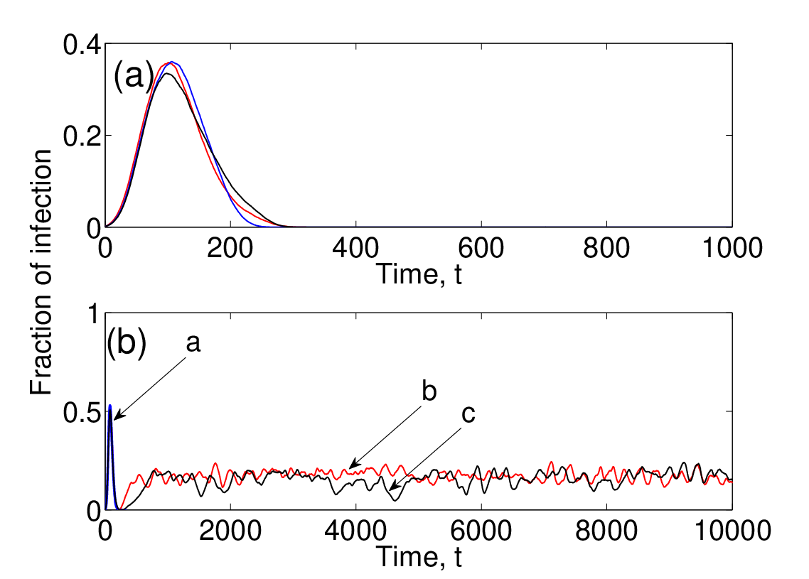
Next, we examine the effect of mobility on the regions where the epidemic will extinct when the mobility rate is varied. By using the method developed in literature [59], we know that this scenarios can be distinguished by computing the probability when the epidemic has gone extinct after a waiting time . For illustration, we have considered the fixed parameters and . In Fig. 6, we obtain the dependence of on the mobility rate . With increasing mobility rate, the extinction probability with a sharpened transition emerges at a critical value for the entire lattice area explored in 10000 time-unit. One could see that, above , the extinction probability tends to zero as the mobility rate increase, and the epidemic is stable persistence (implying super-persistent transients [86]). On the other hand, below the critical mobility rate , the extinction probability approaches 1 for small mobility rate, and the epidemics occurs is unstable. One of our central results is that we have identified a mobility threshold for persistence of epidemics. Without loss of generality, we also have tested the data for the other parameters values and , the same sharpened transitions have been observed from the lattice simulations.
There exists a critical value such that a high mobility changes the extinction phase to persistence phase, while remains extinction, leaving a uniform state with only susceptible in entire space. It is worth noting that our above results arise from the domain I of extinction phase in Fig. 2 where and absence of mobility. Therefore, our results also indicate that the stronger mobility can increase the parameter region where the epidemic persistence occurs. This may be completely explained from the local and global infection [61]. The higher mobility leads to a increasing of the global contact among individuals in the lattices.

Reichenbach et al had assessed the effects of mobility on the spatial pattern of rock-paper-scissors games [59]. Results demonstrated that a critical influence of mobility on species diversity: when mobility exceeds a certain value, biodiversity is jeopardized and lost. In contrast, below this critical threshold all subpopulations coexist and an entanglement of traveling spiral waves forms in the course of time. In our study, we incorporate the scenarios outlined in Refs. [59, 87] and also investigate a spatial pattern induced by mobility when the parameters are within domain II of Fig. 2. We perform extensive computer simulations of the stochastic system (see Eqs. (1) and (3)) and typical snapshots of the steady states are shown in Fig. 7. With increasing mobility , these moving spiral structure grow in size and saturate at a certain value, but they don’t disappear with respect time. This is different from rock-paper-scissors games where the spiral wave will disappear for large mobility [59]. As shown in Fig. 7, the spirals’ wavelength rises with the individuals’ mobility increased. When the parameters are within domain I, we have not observed the spatial pattern emergence for varied mobility rate . However, we find that the high mobility lead to entire disease outbreaks instead of localized disease outbreaks (see Fig. 8).
From the above observations we know that the mobility of individuals can dramatically affect the epidemics extinction/persistence and spatial pattern. We need to point out here that, although our results in this study come from cellular automata’s simulation, it is also useful for assessing the dynamics of deterministic systems, such as stochastic PDEs, spatial correlation models, ordinary difference equation, and so forth [59, 83, 70, 12, 88, see]. By modeling the interaction among individuals, we are able to understand the role of spatial mixed (cause by mobility) in invasion dynamics without the need for complex mathematical methods. Whether an organism can successfully invade and persist in the long-term is dependent on many factors. Here, we have identified a mobility factor for epidemic persistence and invasion, which is distinguished from the nonlinear dynamics of the epidemic models.
(a) (b)
(b)
(a)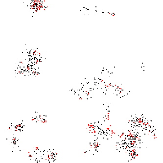 (b)
(b)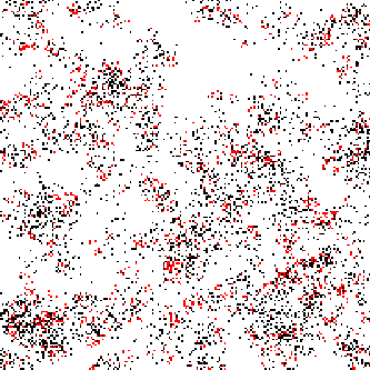
III.3 Spatio-temporal synchronous dynamics of spatial epidemics
As individuals travel around the world for human, as well as migrate for animals, the disease may spread from one place to another. The spatial spread of epidemics has been much studied, particularly with respect to pandemic invasion waves [2, 5, 6, 89, 90, 91]. Simulation models incorporating transportation have generated important insights into the spread of epidemics. However, the key underlying relationship between human movement and disease spread has not been verified across wide spatial scales. To quantify the traveling behavior of individuals, we consider the linked dynamics of two host communities each of size , where individuals possess mobility in each patch. Spatial coupling is the critical parameter determining phase coherence and spatial synchrony [18] and the persistence of host-pathogen systems [92, 93]. For simplicity, we assume that is constant through time for each patch. The typical schematic for two patches is shown in Fig. 9.

Consider now, two patches with sizes cells each other, each representing a community or suburb, and suppose a small number of infective individuals in each community at initial time. The individual can pass from one community to the other. This migration or the individual traveling is randomly chosen for some given individuals moving from a community to another community in the large metapopulation systems. The strength of coupling between the two communities is measured by
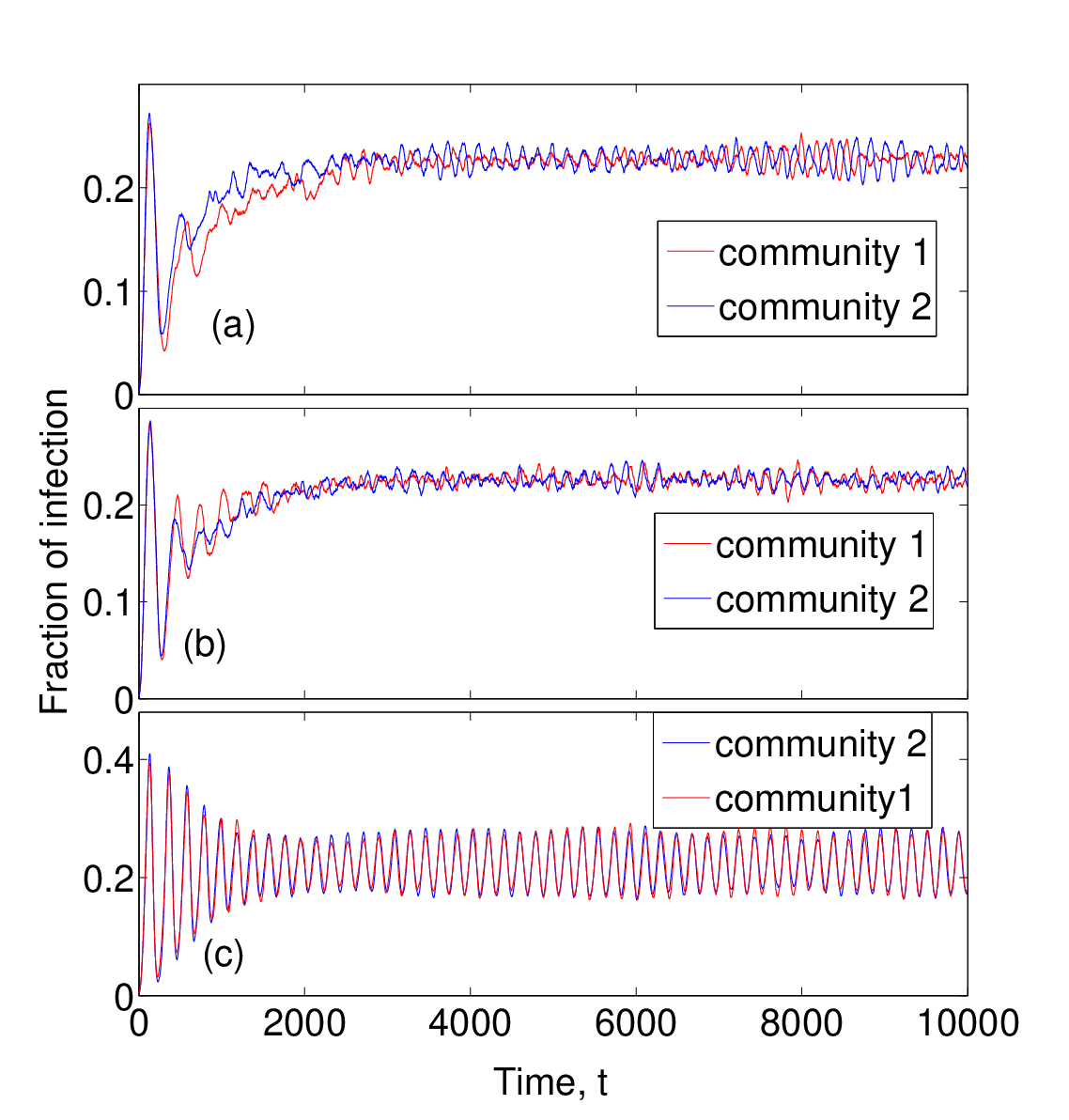
| (4) |
with respect to unit time. Although the approach is only a rough approximation of the dynamic nature of transportation between two communities, it nevertheless capture some of the essential elements [3, 94]. Figure 10 shows a simulation results with different coupling strength between two communities, in which the mobility within patch is ignored. In this case, the infectives in each community are seen to irregular oscillate and local anti-phase for weak coupling strength (see Fig. 10(a) and (b)). Upon increasing the coupling strength between the communities, the suburbs show in-phase synchronization 22 2 Note that here the synchronization or asynchronization refers to oscillate with Uniform Phase evolution, yet has Chaotic Amplitudes(UPCA). In addition, the synchronization can be quantified by calculating the phase of each time-series of infectives and plotting the phase difference between the two suburbs [103, 104, 18]. (see Fig. 10(c)). Notice that the similar results have been obtained by using SIRS network model [3, 21]. As previous subsection’s results show that, at the single patch level, the epidemic behavior on the global 33 3 Here, the global refers to as the single patch, rather than the metapopulation system. scale is also determined by the mobility of individuals. In particular, the effects due to the finite size of communities and the stochastic nature of the mobility might have a crucial role in the problem of resurgent epidemics, extinction and eradication [95, 96, 97, 94, also see]. Therefore it is important to consider the effect of mobility rate on synchronization for the metapopulation system. In Fig. 11, we report the effect of different mobility rate on the time-series of infected fraction by the lattice simulations. Figure. 11 provides a clear evidence of the spatio-temporal synchrony in metapopulation system independent of the self-mobility, but it depends on the coupling strength among patches. One can draw a conclusion that mobility within each patch does not play a signification role, and spatial structure within patches can be ignored when investigate the coupling patches.
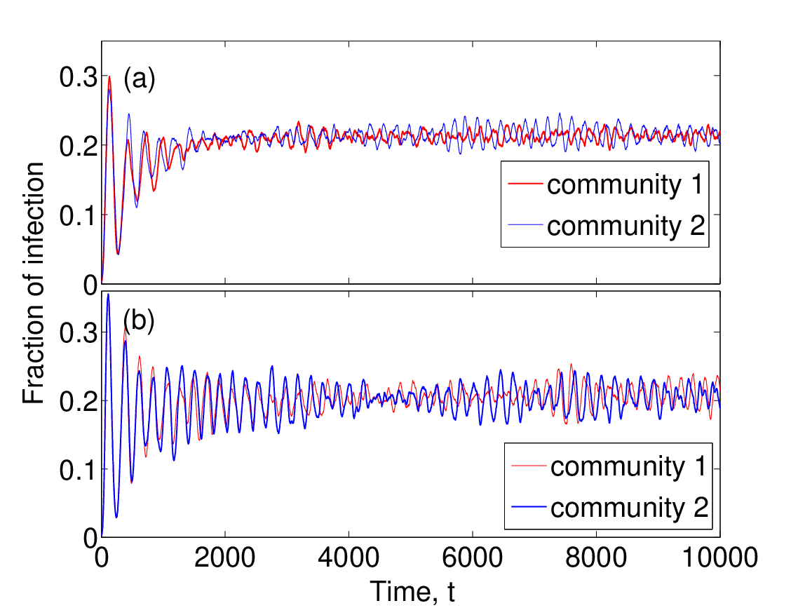
One of our main goals is to study the manner in which two or more communities or suburbs synchronize in time, as recurring waves of infection sweep through their respective populations by means of cellular automata simulation. This is a fascinating outcome of spatial dynamics whereby a few migrating infective individuals have the potential to spread the epidemic from one community to the other, giving rise to synchrony in the long term. For instance, the time-series of measles infections in various cities of England (1944–1958) are reported in literatures [18, 3, 98]. The Birmingham and Newcastle appear to synchronize in-phase together while Cambridge and Norwich are clearly out of phase by 180 degree (see Fig. 12 in Appendix and Fig. 2 in literature [18, 98]). Here, we simulate a simple coupled spatial community models to gain insights about the coupling strength. These results provide useful insights for the basic theoretical understanding of mechanistic epidemic models in complex multi-patches environments, which can then be used to build more realistic data-driven large-scale computational approaches for real case scenarios and spatially targeted control measures. For instance, the spread of influenza shows spatial synchrony in 49 states of United Sates [2].
IV Conclusions and discussion
As a summary, from the simulations of individuals’ spreading processes among lattices with randomly distributed in the space, we can identify different effects of parameters describing the spatial structure and the temporal developments of disease for individuals, such as , , , and , on the dynamical behavior–persistence, extinction and synchrony. We change every parameter which we consider can affect the spreading process. Although the short-term behavior (persistence and extinction) may depend on system size and details of spatial distribution, the long-term behavior mainly depends on three parameters: the infection period , infection rate , and mobility for single community. The two former parameters determine what types spatial pattern emerge, and the last dramatically increase the parameters region where the epidemics pandemic occurs in the space. Moreover, we investigate the coupling between multi-community, in which the two former parameter and reflect the nature of the developing and pandemic period of disease for individuals, the coupling strength is a parameter related to the population density, the frequencies of people contacts, and the extent of people traveling between different places or cities [93]. These results may be helpful for the analysis of the spreading processes of diseases in space.
The possibility of spiral waves, self-organized spatial pattern, spotted pattern, traveling wave as well as trade-offs in spatial epidemics and host-parasitoid by local dispersal abilities has long been recognized [99, 100, 1, 15, 24, 23, 2, 18]. What is new here is that the trade-off between persistence and extinction have been understood in the spatial structure epidemics model. The discrete character of the individuals involved in the reactions (1) and the mobility processes (3) are responsible for intrinsic stochasticity arising in the system. Individuals’ mobility as well as intrinsic noise have crucial influence on the self-formation of spatial patterns. The analytical expressions for the spirals’ wavelength as function of mobility can be determined by means of a complex Ginzburg-Landau equation (CGLE) obtained by recasting the PDE derived from interacting particle approach [70, 59]. Hence, to qualitatively explain these findings, a profound understanding is still desirable and could motivate further investigations.
Acknowledgments
We are grateful for the constructive suggestions of the two anonymous referees on our original manuscript. We thank Bai-Lian Li for improving the English on the original manuscript.
This work was supported by the National Natural Science Foundation of China under Grant No. 60771026, Program for New Century Excellent Talents in University (NCET050271), and the Natural Science Foundation of Shan’xi Province Grant No. 2007021006.
Appendix A
We give here the time series of weekly measles case reports for Birmingham and Newcastle between 1948 and 1969, which exhibits in-phase pattern.

References
- [1] W. M. van Ballegooijen and M. C. Boerlijst, Proc. Natl. Acad. Sci. USA 101, 18246 (2004).
- [2] C. Viboud, O. N. Bjornstad, D. L. Smith, L. Simonsen, M. A. Miller, and B. T. Grenfell, Science 312, 447 (2006).
- [3] D. He and L. Stone, Proc. R. Soc. Loand. B 270, 15919 (2003).
- [4] H. T. H. Nguyen and P. Rohani, J. R. Soc. Interface 5, 403 (2008).
- [5] Y. Xia, O. Bjornstad, and B. Grenfell, Am. Nat. 164, 267 (2004).
- [6] D. J. D. Ear, P. Rohani, and B. T. Grenfell, Proc. R. Soc. Lond. B 265, 7 (1998).
- [7] M. Heino, V. Kaitala, E. Ranta, and J. Lindstrom, Proc. R. Soc. Lond. B 264, 481 (1997).
- [8] B. Bolker and B. Grenfell, Phil. Tran. R. Soc. B 348, 309 (1995).
- [9] D. J. Earn, P. Rohani, B. M. Bolker, and B. T. Grenfell, Science 287, 667 (2000).
- [10] S. A. Frank, Evol. Ecol. 5, 193 (1991).
- [11] D. A. Rand, M. Keeling, and H. B. Wilson, Proc. R. Soc. Lond. B 259, 55 (1995).
- [12] M. J. Keeling, Proc. R. Soc. Lond. B 266, 859 (1999).
- [13] M. J. Keeling, S. P. Brooks, and C. A. Gilligan, Proc. Natl. Acad. Sci. USA 101, 9155 (2004).
- [14] H. Fukś, A. T. Lawniczak, and R. Duchesne, Eur. Phys. J. B 50, 209 (2006).
- [15] Q.-X. Liu, Z. Jin, and M.-X. Liu, Phys. Rev. E 74, 031110 (pages 6) (2006).
- [16] M. Boots and A. Sasaki, Proc. R. Soc. Lond. B 266, 1933 (1999a).
- [17] M. Kamo, A. Sasaki, and M. Boots, J. Theor. Biol. 244, 588 (2007).
- [18] B. T. Grenfell, O. N. Bjørnstad, and J. Kappey, Nature 414, 716 (2001).
- [19] V. Colizza, A. Barrat, M. Barthelemy, and A. Vespignani, Proc. Natl. Acad. Sci. USA 103, 2015 (2006).
- [20] L. Stone, R. Olinky, and A. Huppert, Nature 446, 533 (2007).
- [21] M. Kuperman and G. Abramson, Phys. Rev. Lett. 86, 2909 (2001).
- [22] F. Jeltsch, M. S. Muller, V. Grimm, C. Wissel, and R. Brandl, Proc. R. Soc. Lond. B 264, 495 (1997).
- [23] G. Sun, Z. Jin, Q.-X. Liu, and L. Li, J. Stat. Mech.: Theory and Exper. 2007, P11011 (2007).
- [24] Q.-X. Liu and Z. Jin, J Stat. Mech.: Theory and Exper. 2007, P05002 (2007).
- [25] A. Gautreau, A. Barrat, and M. Barthélemy, J Stat. Mech.: Theory and Exper. 2007, L09001 (2007).
- [26] R. Pastor-Satorras and A. Vespignani, Phys. Rev. Lett. 86, 3200 (2001).
- [27] A. L. Lloyd and R. M. May, Science 292, 1316 (2001).
- [28] N. M. Ferguson, M. J. Keeling, W. John Edmunds, R. Gani, B. T. Grenfell, R. M. Anderson, and S. Leach, Nature 425, 681 (2003).
- [29] S. Eubank, H. Guclu, V. S. A. Kumar, M. V. Marathe1, A. S. abd Zoltán Toroczkai, and N. Wang, Nature 429, 180 (2004).
- [30] D. L. DeAngelis and L. J. Gross, Individual-based models and approaches in ecology: populations, communities and ecosystems (Chapman and Hall, New York, London, 1992).
- [31] N. Boccara and K. Cheong, J. Phys. A: Math. and Gen. 25, 2447 (1992).
- [32] N. Boccara and K. Cheong, J. Phys. A: Math. and Gen. 26, 3707 (1993).
- [33] N. Boccara, O. Roblin, and M. Roger, Phys. Rev. E 50, 4531 (1994).
- [34] R. Durrett, SIAM Review 41, 677 (1999).
- [35] J. A. Sherratt, B. T. Eagan, and M. A. Lewis, Philos. Trans. R. Soc. Lond. B 352, 21 (1997).
- [36] S. L. Lima and P. A. Zollner, Trends Ecol. Evol. 11, 131 (1996).
- [37] P. Schippers, J. Verboon, J. P. Knaapen, and R. C. van Apeldoorn, Ecography 19, 97 (1996).
- [38] F. R. Adler, Am. Nat. 141, 642 (1993).
- [39] J. C. Allen, W. M. Schaffer, and D. Rosko, Nature 364, 229 (1993).
- [40] B. T. Grenfell and J. Harwood, Trends Ecol. Evol. 12, 395 (1997).
- [41] B. Bolker, Bull. Math. Biol. 61, 849 (1999).
- [42] J. D. Murray, Mathematical Biology (Springer, Berlin, 1993).
- [43] M. Lewis, J. Renclawowicz, and P. van den Driessche, Bull. Math. Biol. 68, 3 (2006).
- [44] A. Gautreau, A. Barrat, and M. Barthélemy, J. Theor. Biol. 251, 509 (2008).
- [45] R. M. Anderson and R. M. May, Infectious Diseses of Humans (Oxford University Press, Oxford, 1991).
- [46] F. Brauer and C. Castillo-Cháavez, Mathematical Models in Population Biology and Epidemiology (Springer-Verlag, New York, 1996).
- [47] A. F. Rozenfeld and E. V. Albano, Phys. Rev. E 63, 061907 (2001).
- [48] T. Antal and M. Droz, Phys. Rev. E 63, 056119 (2001).
- [49] A. Antoniazzi, D. Fanelli, S. Ruffo, and Y. Y. Yamaguchi, Phys. Rev. Lett. 99, 040601 (2007).
- [50] C. J. Tessone, M. Cencini, and A. Torcini, Phys. Rev. Lett. 97, 224101 (2006).
- [51] Z.-J. Tan, X.-W. Zou, and Z.-Z. Jin, Phys. Rev. E 62, 8409 (2000).
- [52] E. M. Rauch and Y. Bar-Yam, Phys. Rev. E 73, 020903 (2006).
- [53] A. S. Julian Adamek, Michael Keller and H. Hinrichsen, J. Stat. Mech.: Theor. and Exper. 2005, P09002 (2005).
- [54] A. F. Rozenfeld and E. V. Albano, Phys. Lett. A 332, 361 (2004).
- [55] A. F. Rozenfeld, C. J. Tessone, E. V. Albano, , and H. S. Wio, Phys. Lett. A 280, 45 (2001).
- [56] S. Petrovskii and B.-L. Li, J. Theor. Biol. 212, 549 (2001).
- [57] M. Mobilia, I. T. Georgiev, and U. C. Täuber, Phys. Rev. E 73, 040903 (2006).
- [58] A. L. Lloyd, Theor. Popul. Biol. 65, 49 (2004).
- [59] T. Reichenbach, M. Mobilia, and E. Frey, Nature 448, 1046 (2007a).
- [60] T. Reichenbach, M. Mobilia, and E. Frey, Phys. Rev. E 74, 051907 (2006).
- [61] M. Boots and A. Sasaki, Proc. R Soc. Lond. B 266, 1933 (1999b).
- [62] M. Boots and A. Sasaki, Ecol. Lett. 6, 176 (2003).
- [63] M. S. Bartlett, Proceedings of the Third Berkeley Symposium on Mathematics, Statistics and Probability (University of California Press, Berkeley, 1956), vol. 4, chap. Deterministic and stochastic models for recurrent epidemics, pp. 81–109.
- [64] M. S. Bartlett, J. R. Statist. Soc. Ser. A 120, 48 (1957).
- [65] M. S. Bartlett, J. R. Statist. Soc. Ser. A 123, 37 (1960).
- [66] I. Nasell, J. R. Stat. Soc. Ser. B 61, 309 (1999a).
- [67] I. Nasell, Theor. Popul. Biol. 67, 203 (2005).
- [68] D. Alonso, A. J. Mckane, and M. Pascual, J. R. Soc. Interface 4, 575 (2006).
- [69] M. Simoes, M. M. T. da Gama, and A. Nunes, J. R. Soc. Interface 5, 555 (2008).
- [70] T. Reichenbach, M. Mobilia, and E. Frey, J. Theor. Biol. 254, 368 (2008), arxiv:0801.1798.
- [71] R. P. Boland, T. Galla, and A. J. McKane, J. Stat. Mech. 2008, P09001 (2008).
- [72] I. Nasell, J. Theor. Biol. 211, 11 (2001).
- [73] I. Nasell, Math. Bios. 156, 21 (1999b).
- [74] J. C. Claussen and A. Traulsen, Phys. Rev. Lett. 100, 058104 (pages 4) (2008).
- [75] F. van den Bosch, J. Zadoks, and J. Metz, Phytopathology 78, 54 (1988).
- [76] F. van den Bosch, J. A. J. Metz, and J. C. Zadoks, Phytopathology 89, 495 (1999).
- [77] M. E. J. Newman, Phys. Rev. E 66, 016128 (2002).
- [78] J. M. Read and M. J. Keeling, Proc. R. Soc. Lond. B 270, 699 (2003).
- [79] B. Bolker and S. W. Pacala, Theor. Popul. Biol. 52, 6 (1997).
- [80] U. Dieckmann, R. Law, and J. A. J. Metz, The Geometry of Ecological Interactions: Simplifying Spatial Complexity (Cambridge University Press, Cambridge, 2000).
- [81] J. Medlock and M. Kot, Math. Biosci. 184, 201 (2003).
- [82] S. Harris and W. J. Trewhella, J. Appl. Ecol. 25, 409 (1988).
- [83] T. Reichenbach, M. Mobilia, and E. Frey, Phys. Rev. Lett. 99, 238105 (pages 4) (2007b).
- [84] D. T. Gillespie, J. Phys. Chem 81, 2340 (1977).
- [85] D. T. Gillespie, J. Chem. Phys. 113, 297 (2000).
- [86] A. Hastings, Trends Ecol. Evol. 19, 39 (2004).
- [87] T. L. Czaran, R. F. Hoekstra, and L. Pagie, Proc. Natl. Acad. Sci. USA 99, 786 (2002).
- [88] D. Ebert, M. Lipsitch, and K. L. Mangin, Am. Nat. 156, 459 (2000).
- [89] R. F. Grais, J. H. Ellis, and G. E. Glass, Eur. J. Epidemiol. 18, 1065 (2003).
- [90] L. Hufnagel, D. Brockmann, and T. Geisel, Proc. Natl. Acad. Sci. USA 101, 15124 (2004).
- [91] N. C. Grassly, C. Fraser, and G. P. Garnett, Nature 433, 417 (2005).
- [92] J. Swinton, Bull. Math. Biol. 60, 215 (1998).
- [93] B. Grenfell and B. Bolker, Ecol. Lett. 1, 63 (1998).
- [94] V. Colizza and A. Vespignani, J. Theor. Biol. 251, 450 (2008).
- [95] F. Ball, D. Mollison, and G. Scalia-Tomba, Ann. Appl. Probab. 7, 46 (1997).
- [96] P. C. Cross, J. O. Lloyd-Smith, P. L. F. Johnson, and W. M. Getz, Ecol. Lett. 8, 587 (2005).
- [97] P. C. Cross, P. L. Johnson, J. O. Lloyd-Smith, and W. M. Getz, J. R. Soc. Interface 4, 315 (2007).
- [98] N. Bharti, Y. Xia, O. N. Bjornstad, and B. T. Grenfell, PLoS ONE 3, e1941 (2008).
- [99] H. N. Comins and M. P. Hassell, J. Theor. Biol. 183, 19 (1996).
- [100] M. P. Hassell, H. N. Comins, and R. M. May, Nature 370, 290 (1994).
- [101] R. Kuske, L. F. Gordillo, and P. Greenwood, J. Theor. Biol. 245, 459 (2007).
- [102] J. Dushoff, J. B. Plotkin, S. A. Levin, and D. J. D. Earn, Proc. Natl. Acad. Sci. USA 101, 16915 (2004).
- [103] M. G. Rosenblum, A. S. Pikovsky, and J. Kurths, Phys. Rev. Lett. 76, 1804 (1996).
- [104] B. Blasius and L. Stone, Inter. J Bifur. and Chaos 10, 2361 (2000).