Quantum Private Queries: security analysis
Abstract
We present a security analysis of the recently introduced Quantum Private Query (QPQ) protocol. It is a cheat sensitive quantum protocol to perform a private search on a classical database. It allows a user to retrieve an item from the database without revealing which item was retrieved, and at the same time it ensures data privacy of the database (the information that the user can retrieve in a query is bounded and does not depend on the size of the database). The security analysis is based on information-disturbance tradeoffs which show that whenever the provider tries to obtain information on the query, the query (encoded into a quantum system) is disturbed so that the person querying the database can detect the privacy violation.
pacs
03.67.Lx, 03.67.Dd, 03.67.MnI Introduction
In its most basic form, the scenario we consider can be described as follows. On one side we have a provider, Bob, who controls an ordered classical database composed of memory cells. Each cell of the data-base contains an bit string, so that the database consists of strings . On the other side, we have the person querying the database, Alice, who wants to recover the string associated with a memory cell (say the -th one) but at the same time does not want Bob to know which cell she is interested in (user privacy). In a purely classical setting the simplest strategy for Alice consists in placing a large number of decoy queries, i.e. she “hides” her query among a large number of randomly selected queries. In this case, she will be able to get the information she is looking for, while limiting Bob’s intrusion in her privacy. [In fact, the mutual information between Alice’s true query and Bob’s estimate of such value is upper bounded by ]. The drawbacks associated with such procedures are evident. First of all, the method does not allow Alice to check whether Bob is retaining information on her queries. Moreover, to achieve a high level of privacy Alice is forced to submit large amounts of fake queries, increasing the communication cost of the transition: in particular, absolute privacy is obtained only for , i.e. by asking Bob to send all his database. This may not be acceptable if the database is huge or if it is an asset for Bob (data privacy).
User and data privacy are apparently in conflict: the most straightforward way to obtain user privacy is for Alice to have Bob send her the entire database, leading to no data privacy whatsoever. Conversely, techniques for guaranteeing the server’s data privacy typically leave the user vulnerable [1]. At the information theoretical level, this problem has been formalized as the Symmetrically-Private Information Retrieval (SPIR) [1] generalizing the Private Information Retrieval (PIR) problem [2, 3] which deals with user privacy alone. SPIR is closely related to oblivious transfer [4], in which Bob sends to Alice bits, out of which Alice can access exactly one–which one, Bob doesn’t know. No efficient solutions in terms of communication complexity [5] are known for SPIR. Indeed, even rephrasing them at a quantum level [6, 7], the best known solution for the SPIR problem (with a single database server) employs qubits to be exchanged between the server and the user, and ensures data privacy only in the case of honest users (i.e. users who do not want to compromise their chances of getting the information about the selected item in order to get more). Better performance is obtained for the case of multiple non-mutually communicating servers [2] (although the user cannot have any guarantee that the servers are not secretly cooperating to violate her privacy), while sub-linear communication complexity is possible under the some computational complexity assumption, e.g. [3]. PIR admits protocols that are more efficient in terms of communication complexity [2, 3].
The Quantum Private Queries (QPQ) protocol we have introduced in Ref. [8] is a cheat sensitive strategy [9] which addresses both user and data privacy while allowing an exponential reduction in the communication and computational complexity with respect to the best (quantum or classical) single-server SPIR protocol proposed so far. Specifically QPQ provides a method to check whether or not Bob is cheating and does not need the exchange of the whole database (i.e. qubits): in its simplest form it only requires Bob to transfer two database elements, identified by qubits, for each query. The QPQ protocol is ideally composed by a preliminary signaling stage where the user and the database provider exchange some quantum messages (specifically Alice addresses Bob receiving some feedback from him) and by a subsequent retrieval&check stage where Alice performs some simple quantum information processing on the received messages to recover the information she is interested in and to check Bob’s honesty. The QPQ security relies on the fact that if Bob tries to infer the query Alice is looking for, she has a nonzero probability of discovering it. Most importantly, one can verify that the more information Bob gets on Alice query, the higher is the probability that he will not pass Alice’s honesty test. In this paper we will derive analytical bounds for such a theoretical trade-off, and we analyze different variants of the QPQ protocol.
The main idea behind the protocol is the following. Alice submits her request to Bob using some quantum information carrier, so that she can either submit a plain query or a quantum superposition of different queries . Alice randomly alternates superposed queries and non-superposed queries. Thus, Bob does not know whether the request he is receiving at any given time is a superposition of queries or not, so that he does not know which measurement will leave the information carrier unperturbed: he cannot extract information without risking to introduce a disturbance that Alice can detect. Bob can, however, respond to Alice’s request without knowing which kind of query was submitted. His response will be either of the form or of the form , where the first ket is the register that Alice had sent him, the second ket is a register that contains Bob’s answer ( being the answer to the th query), and which may be entangled with the first. From these answers Alice can both obtain the reply to her query and check that Bob has not tried to breach her privacy.
The main assumption we adopt is that, for each , there exists a unique answer string that can be independently checked by Alice. [This does not prevent different queries from having the same answer: indeed we do admit the possibility to have for .] For example, Alice may be asking Bob the prime factors of one out of very large integer numbers (say the RSA collection) which she cannot factorize by herself. The above requirements can be relaxed (examples will be provided in Sec. VII), but they are useful as they permit a considerable simplification of the security proof. For the same reason, we will focus on the simplest version of the QPQ protocol, where there exists a reference query (dubbed rhetoric query) which has a known standard answer . As discussed in Ref. [8], this assumption is not fundamental, but it is very useful since it allows us to minimize the amount of exchanged signals in the protocol (as a matter of fact alternative versions of the QPQ protocol with higher security level can be devised which do not employ the rhetoric query).
The paper is organized as follows. In Sec. II we describe the rhetoric version of QPQ in its basic form and introduce the notation. This is followed by the technical Sec. III where we analyze in detail the most general transformations Bob can perform on Alice’s queries. Section IV contains the main result of the paper: here we introduce the trade-off between Bob’s information on Alice’s query and the success probability of him passing her honesty test. In Sec. V we present some variations of the QPQ protocol, one of which exploits entanglement as a resource to strengthen Alice’s privacy. Finally in Sec. VI we analyze what happens when relaxing some of the assumptions adopted in the security proof. In particular we show that the basic version of the QPQ described here does not guarantee privacy if the queries have multiple answers, and we point out a possible solution in Sec. VII.
II Preliminaries and notation
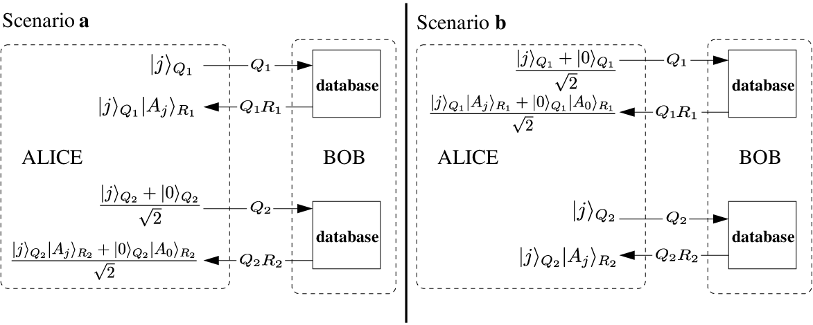
In the rhetoric version of the QPQ protocol (see Fig. 1) Alice uses two quantum registers each time she needs to interrogate Bob’s database. The first register contains , the address of the database memory cell she is interested in; the other register is prepared in a quantum superposition of the type , “” being the rhetoric query. Alice then secretly and randomly chooses one of the two registers and sends it to Bob. He returns the register Alice has sent to him, together with an extra register in which the corresponding answer is encoded. In order to reply to Alice’s query without knowing whether it is the superposed query or not, Bob needs to employ the quantum random access memory (qRAM) algorithm [10, 11]. After Alice has received Bob’s first reply, she sends her second register and waits for Bob’s second reply. Again Bob returns her register together with an extra register which encodes his reply obtained through a qRAM application. If Bob has followed the protocol accurately, without trying to extract information, Alice now should possess a state which encodes the information she is looking for and an entangled state involving the rhetoric query, whose coherence can be tested to check Bob honesty, i.e. the two states and . Alice recovers the value of by measuring the second register in the first state, and then she uses this value to prepare a measurement to test whether the superposition has been retained in the second state (“honesty test”). Such a measurement is simply a projective measurement on the state . If this test fails, namely if she finds out that the state Bob has sent her back is orthogonal to the one she is expecting, she can be confident that Bob has cheated and has violated her privacy. If, instead, the test passes, she cannot conclude anything. In fact, suppose that Bob has measured the state and collapsed it to the form or to the form , it still has a probability 1/2 to pass Alice’s test of it being of the form . So Alice’s cheat test allows her to be confident that Bob has cheated if the test fails, but she can never be completely confident that Bob has not cheated if the test passes.
We now introduce the notation which will be used. We define the source space which contains the addresses of the memory cells which compose Bob’s database, identifying with the address of the rhetoric query. For each we define to be the information associated with the -th address. As mentioned in the introduction the are classical messages composed of bits, and they need not represent distinct messages (i.e. we allow the possibility that for ), but they are uniquely determined by the value of . In this context, Bob’s database is defined as the ordered set formed by the strings . We define the two quantum registers Alice uses to submit her queries; according to the protocol, she will first send , wait for Bob’s answer and then send . In this notation, for , the vector is the state of the -th register which carries the address of the -th database memory. For all we use the vector to represent the superposition of the -th query and the rhetoric query, i.e.
| (1) |
(for we have ). We define the registers on which Bob writes the information to send back to Alice. After having received from Alice, Bob encodes the necessary information on and sends back to her both and . Analogously, after having received , he will encode information on and send her back both and . It is useful to also define the vectors
| (2) | |||||
| (3) |
(as in Eq. (1) for we set ). According to the protocol, the vectors or are the states that an honest Bob should send back to Alice when she is preparing into the states or , respectively. In fact, the states and are the result of the qRAM transformation when it is fed and , respectively. We also introduce an ancillary system to represent any auxiliary systems that Bob may employ when performing his local transformation on the Alice queries, plus (possibly) an external environment.
Let us use this notation to better formalize the QPQ protocol described above. Suppose then that Alice wants to address the -th entry of the database. The protocol goes as follows:
- 1.
Alice randomly chooses between the two alternative scenarios a and b (see Fig. 1). In the scenario a, she prepares the qubits in and the qubits in . Instead, in the scenario b she prepares the states and . This means that, in the scenario a, she first sends the plain query and then the superposed query. On the contrary, in the scenario b, she first sends the superposed query and then the plain query. Consequently, the input state of the system is described by the vectors
where the index refers to the selected scenario and is the fiducial initial state of the systems and (it is independent on because Bob does not know which scenario Alice has chosen).
- 2.
Now Alice sends and waits until Bob gives her back and . Then, she sends and waits until she gets back and .
- 3.
Honesty Test: Alice checks the states she has received. If she had selected scenario a, she performs a von Neumann measurement to see if is in the state — see Eq. (3). Of course, this can be done in two steps: first she measures to learn and then she uses this value to prepare an appropriate measurement on . If the measurement fails, then Alice can definitely conclude that Bob was cheating, otherwise she can assume he was honest (although she has no guarantee of it). If she had chosen scenario b, she proceeds analogously, using a von Neumann measurement to check if is in the state .
III Bob’s transformations
In the QPQ protocol, Alice’s privacy relies essentially on the fact that Bob is not allowed to operate jointly on and . This a fundamental constraint: without it, Bob would be able to discover the index without Alice knowing it. In fact, the subspaces spanned by the two vectors and (associated to the two different scenarios a and b for the query ) are mutually orthogonal. Thus, such vectors (and then the corresponding queries) could be easily distinguished by performing on a simple von Neumann measurement defined by the projectors associated with the spaces . This is a measurement that would allow Bob to recover Alice’s query without disturbing the input states of . To prevent this cheating strategy, the QPQ protocol forces Bob to address and separately (i.e. he has to send the register back, before Alice provides him the register ).
Bob’s action when he receives Alice’s first register can be described by a unitary operator which acts on the first register , on , and on (and not on the second register which is still in Alice’s possession). Analogously, Bob’s action when he receives the second register is described by the unitary operator which acts on , , and (and not on and which are now in Alice’s possession). [Note that the above framework describes also the situation in which Bob is employing non-unitary transformations (i.e. CP-maps), since the space can be thought to contain also the Naimark extension that transforms any CP-map into a unitary.] The above transformations cannot depend on the selected scenario (as Bob does not know which one, among a and b, has been selected by Alice). Therefore, within the th scenario, the global state at the end of the protocol is described by the vectors
| (8) |
with given in Eq. (1).
III.1 Some useful decompositions
Consider the transformation . In the scenario a for all we can write
| (9) | |||
where stands for the separable state and where is a vector orthogonal to , i.e.
| (10) |
With this choice, is the probability that the state (9) will be found in . In the scenario b, instead, for we can write
| (11) | |||
As before and is a vector orthogonal to the “check state” Alice is expecting, i.e.
| (12) |
Consequently is the probability that the state (11) will pass the test of being in . The state on the first line of Eq. (11) can be expanded on a basis of which the state on the first line of Eq. (9) is a component. Therefore and must be related. The security analysis given in the following sections is based on the study of this relation.
Analogous decompositions can be given for : in this case, however, it is useful to describe them not in terms of the input states, but in terms of the state of the system after it has passed the test on the subsystems . For , in the scenario a this gives:
| (13) | |||
Here is a vector orthogonal to of Eq. (3) i.e.
Thus is the probability that the state (13) will pass the test of being in . Notice that the vector in the first line of Eq. (13) is the state of one obtains in the scenario a if, after the first round, the state passes the test of being — see Eq. (9). In the scenario b, instead, we have
| (14) | |||
where is a vector orthogonal to the state , i.e.
and is the probability that the state (14) will be found in .
The case has to be treated separately: indeed, if Alice sends this query then both and will be prepared into . In this case, it is then useful to define by considering its action on the vector with defined as in Eq. (9), i.e.
| (15) | |||
where again one has
From the above equations, it follows that for the final state (8), after Bob has finished his manipulations, can be written as follows for scenario a
| (16) |
where all the terms in the second and third line are orthogonal to . Analogously, we have for scenario b
| (17) |
where, again, the states in the last two lines are orthogonal to the state in the first. Instead, for we have
| (18) |
IV Information-disturbance tradeoff and Privacy
In this section we present an information-disturbance analysis of the QPQ protocol. This will yield a trade-off which shows that, if Bob tries to get some information on Alice’s queries, then she has a nonzero probability of detecting that he is cheating. The same analysis can be easily reproduced for more complicated versions of the protocol. For instance Alice may hide her queries into superpositions of randomly selected queries. In this case, the derivation, although more involved, is a straightforward generalization of the one presented here.
According to Eq. (8), to measure Bob’s information gain, it is sufficient to study how the final state of the ancillary subsystem depends upon Alice’s query . Exploiting the decompositions introduced in Sec. III we can then show that one can force to keep no track of Alice’s query by bounding the success probabilities that Bob will pass the QPQ honesty test. Specifically, indicating with the success probability associated with Alice’s query in the -th scenario and defining the corresponding output state of , in Sec. IV.1 we will prove the following theorem
Theorem: Choose so that for all and . Then there exists a state of and a positive constant such that the fidelities [12] are bounded as follows,
| (19) |
for all all and .
This implies that, by requiring Bob’s probabilities of passing the honesty test to be higher than a certain threshold , then the final states of will be forced in the vicinity of a common fixed state , which is independent from the choice of and . This in turn implies that, for sufficiently small values of , Bob will not be able to distinguish reliably between different values of using the states in his possession at the end of the protocol. In particular, if , i.e. if Bob wants to be sure that he passes the honesty test, then the final states for any choice of will coincide with , i.e. they will be completely independent from : he cannot retain any memory of what Alice’s query was. It is also worth noticing that since the total number of queries, as well as the number of scenarios , is finite and randomly selected by Alice, then the requirement on in the theorem can be replaced by a similar condition on the average probability of success11 1 Since the number of entries is finite, the condition can be imposed by requiring a similar condition on the average probability . Indeed assume and let be the minimum of the for all and . Since there are terms each contributing to with probability , we have that gives . The condition then follows by taking ..
In Sec. IV.2 we will employ the above theorem to bound the mutual information [13] that connects the classical variable , which labels Alice’s query, and Bob’s estimation of this variable. Assuming that initially Bob does not have any prior information on the value of that Alice is interested in, we will determine the value at the end of the protocol, showing that this quantity is upper-bounded by the parameter of Eq. (19). Specifically, we will show that by requiring that Bob passes the honesty test with a probability greater than , then Alice can bound Bob’s information as
| (20) |
being the number of database entries: his information is upper bounded by a quantity that depends monotonically on a lower bound to his probability of passing the honesty test. Thus, if he wants to pass the honesty test with high probability, he must retain a low information on Alice’s query.
IV.1 Proof of the Theorem
Assume that Alice randomly chooses the scenarios a and b with probability . From Eqs. (16) and (17) it is easy to verify that the success probability that Bob will pass the honesty test when Alice is submitting the -th query is
| (21) |
where and refer to the success probabilities in the scenarios a and b, respectively (these expressions hold also for by setting ). The corresponding output density matrices of the ancillary system is given by
| (22) |
where, for a and b, the state are obtained by partial tracing on Alice’s spaces the output vectors of Eqs. (16) and (17), i.e.
| (23) | |||||
| with | |||||
| (24) | |||||
| (25) |
The quantities (for a and b) are the density matrices obtained by projecting into the state of which allows Bob to pass the honesty test (i.e. for a and for b ).
In accordance with the theorem’s hypothesis, we consider the case in which the probability of passing the test (21) for an arbitrary is higher than a certain threshold, i.e.
| (26) |
with . We will then prove Eq. (19) by identifying the density matrix with the pure defined as in Eq. (15) and showing that the following condition holds
| (27) |
where is the fidelity [12]. Such inequality is a consequence of the fact that we want Bob to preserve the coherence of the superposition , and at the same time to answer correctly to query . To derive it we use Eq. (23) and the condition (26) to write
| (28) |
To prove Eq. (27) it is then sufficient to verify that for all one has
| (29) |
The derivation is similar to the one used in Ref. [14] and can be split in two parts, which will be derived in the following:
i) First we use Eq. (26) and the definitions (9) and (11) to show that for for all one has
| (30) | |||
| (31) |
ii) Then we use Eqs. (30), (31) and the definitions (13) and (14) to verify that for one has
| (32) | |||
| (33) |
which proves the theorem with .
Derivation of Part i)
The condition (26) implies the following inequalities
| (34) |
for all . To obtain inequality (30), we compare Eqs. (9) and (11) under the constraint imposed by Eqs. (34). In particular, we notice that for Eq. (9) gives
| (35) |
with
| (36) |
According to Eq. (34), the vector has a norm of the order . This implies that for the vector (35) almost coincides with . Analogously, Eq. (11) and the second inequality of Eq. (34) tell us that for , the state almost coincides with the vector . Combining these two observations, it follows that for the vectors and almost coincide. According to definition (3), this implies that , and must converge for . To make this statement quantitatively precise, evaluate the scalar product between Eqs. (35) and (11), and obtain the identity
| (37) | |||||
It can be simplified by using the following inequalities:
which can be easily derived from Eq. (36) by invoking the orthogonality conditions (12). Replacing the above expressions into Eq. (37) we get
| (38) | |||||
which implies
| (39) | |||||
| (40) |
We are almost there: indeed Eq. (39) coincides with Eq. (31). To derive Eq. (30) we apply the triangular inequality to the vectors , and .
Derivation of Part ii)
The main difference between the set of Eqs. (9), (11) and the set of Eqs. (13), (14) is the fact that, in the former, acts on vectors with fixed component, while, in the latter, operates on vectors whose components may vary with . We can take care of this by replacing and with the constant vector . This is, of course, not surprising, given the inequalities of Eqs. (30) and (31). To see it explicitly, evaluate the scalar product between and . For it gives,
| (41) |
From the inequalities (34) and (31), it then follows that the modulus of must be close to one, i.e.
| (42) |
Proceeding analogously for the vectors and , we obtain
| (43) |
For all we can then write the following decompositions:
| (44) | |||||
| (45) | |||||
where and are vectors orthogonal to and respectively. The inequality (33) can now be derived by taking the scalar product between Eqs. (45) and (15), remembering that is orthogonal to and using Eqs. (34) and (43). To derive Eq. (32), instead, we first evaluate the scalar product between Eqs. (44) and (45) obtaining
and then we impose the triangular inequality between the vectors , and .
IV.2 A bound on Bob’s information
Here we give an upper bound to Bob’s information on the variable . This can be done by noticing that we can treat as a quantum source which encodes the classical information produced by the classical random source . Specifically, this quantum source will be characterized by the quantum ensemble , where is Alice’s probability of selecting the -th query, and is given by Eq. (22). We can then give an upper bound to Bob’s information by considering the mutual information associated with the ensemble . From the Holevo bound [15], we obtain
| (46) |
where is the average state of , assuming that each of Alice’s queries is equiprobable. To simplify this expression, it is useful to express as
| (47) |
where is the average probability (21) that Bob will pass the test while Alice is sending the -th query, and where and are the density matrices
| (48) | |||
This allows us to write also
| (49) | |||||
| with | |||||
| (50) |
where is Bob’s average probability of passing the honesty test, which, according to Eq. (26), must be greater than . Equations (47) and (49) can then be exploited to produce the following inequalities [10]
| (51) |
where is the binary entropy. Therefore Eq. (46) gives
where is the Holevo information associated with a source characterized by probabilities . This quantity can never be bigger than (the same applies to , but we are not going to use it). Therefore, we can write
| (52) |
which shows that, in the limit in which , the upper bound is only given by . The claim is that for this quantity vanishes. Indeed, according to Eq. (29) we know that for the density matrices converge to the fixed state , hence
| (53) |
More generally, we now show that can be bounded from above to any value for sufficiently close to .
In order to exploit the above relations to give a bound on , let us introduce the probabilities
| (54) | |||
| (55) |
(the inequalities simply follow from Eq. (29)). We can then write
| (56) |
where are density matrices formed by vectors orthogonal to , are traceless operators containing off-diagonal terms of the form , and . We now introduce a unital completely positive trace preserving (CPT) map which destroys the off-diagonal terms while preserving the corresponding diagonal terms, and observe that the von Neumann entropy always increases under the action of a unital map [16]. Therefore,
| (57) | |||||
Now, since is a density matrix in , the quantity can always be upper bounded by with the dimension of . This is not very useful, as can be arbitrarily large. However, a better solution can be obtained. Indeed, we can show that the following inequality holds:
| (58) |
To verify this, we note that the ensemble is composed by density matrices of the form (48) where and are pure vectors satisfying the conditions given in Eq. (29). For small , these vectors are parallel: therefore, there exists a partial isometry connecting to a Hilbert space of dimension which maintains their relative distances intact. Applying such an isometry to all elements of we obtain a new ensemble of , whose elements satisfy to the same relations as the original one. In particular, the two ensembles possess the same value of (in fact, is an entropic quantity, whose value depends only on the relations among the ensemble elements), i.e.
| (59) |
We can now apply to the inequalities (57): the only difference being that now is a density matrix of and hence it satisfies the condition (58). Therefore, we can conclude
Replacing this into (52), we finally find
| (60) |
which thanks to Eq. (55), for sufficiently large yields Eq. (20). This means that Alice can limit Bob’s information , by employing in her tests a value of sufficiently small.
V QPQ variants and entanglement assisted QPQ
In this section we discuss few variants of the QPQ protocol that can be used to improve the security. In particular we introduce an entanglement assisted QPQ in which Alice entangles her registers with a local ancilla before sending them to Bob. As before, we will focus for simplicity on rhetoric versions of such variants, even though similar considerations can be applied also to other (non-rhetoric) QPQ versions.
An example of cheating strategy will allow us to put in evidence the aspects of QPQ that these variants are able to improve. Specifically, suppose that Bob performs a projective measure on all of Alice’s queries to determine the value of the index . As we have seen in the previous section, he will be by necessity disturbing Alice’s state in average, so that she will have some finite probability to find out he is cheating. However, if she had chosen scenario a [see Eq. (1)], then Bob’s first measurement on will return . Now, suppose that his second measurement on Alice’s second request returns the value “0” (this happens with probability ), then Bob will know that Alice had chosen scenario a and that her query was . In this particular case, he will be able to evade detection if he re-prepares the system in the state . [Of course, this does not mean that he will evade detection in general, as this is a situation that is particularly lucky for him, but that has only a small chance of presenting itself. ] A simple variant of the QPQ protocol can be used to reduce the success probability of this particular cheating strategy and in general to strengthen the security of the whole procedure. It consists in allowing Alice to replace the superposition with states of the form , the phase being a parameter randomly selected by Alice. Since Bob does not know the value of , it will be clearly impossible for him to re-prepare the correct reply state after his measurement: as a result his probability of cheating using the simple strategy presented above will be decreased22 2 Analogous improvements are obtained by allowing Alice to replace the states with superposition of the form with the complex amplitudes and being randomly selected.. Furthermore since for each given choice of , the results of Sec. IV apply, one expects that the use of randomly selected s will result in a general security enhancement of the QPQ protocol.
In the previous example, the parameter is a secret parameter whose value, unknown to Bob, prevents him from sending the correct answers to Alice. Another QPQ variant employs entanglement to enhance security. Suppose that, instead of presenting Bob with the states and , as requested by the QPQ protocol, Alice uses the states
| (61) |
where the system is an ancillary system that Alice does not hand over to Bob. The protocol now follows the same procedure as the “canonical” QPQ described previously, but employing the state in place of the state . Of course, Alice’s honesty test must be appropriately modified, as she has to test whether Bob’s actions have destroyed the entanglement between the ancillary system and the register. The main difference with the canonical QPQ is that here half of the times Bob has only access to a part of an entangled state: he is even more limited in re-preparing the states for Alice than in the canonical QPQ. It is easy to see that the security proof given in the previous sections can be straightforwardly extended to this version of the protocol, and that the security bounds derived above still apply: indeed they can be made even more stringent as Bob has only a limited capacity in his transformations on Alice’s queries, since he does not have access to the ancillary space . In the situations in which the information carriers employed in the queries can be put in a superposition of traveling in different directions [17], this version of the protocol can easily be reduced to the canonical QPQ by simply supposing that Alice is in the possession of the database element corresponding to the rhetoric question, while, obviously, Bob is in possession of all the remaining database elements.
VI What if Alice cannot check the answer to her queries independently from Bob?
In deriving the QPQ protocol it is assumed that for each query there is a unique possible answer (notice however that two distinct queries can have the same answer — i.e. can coincides with ). One way to enforce this condition in a realistic scenario is to admit the possibility that Alice can independently verify the answer that Bob is sending to her33 3 This scenario is similar to the one connected to NP problems: the function is difficult to compute for Alice, but once a solution is given to her, she can easily check if it is correct.. In this section we will show that if this is not the case then the basic structure of QPQ does not prevent Bob to cheat without being discovered by Alice. In Sec. VII we will discuss how one can overcome these limitations, at least temporarily, by allowing Alice (or third parties that collaborate with her) to reiterate her query at random times.
VI.1 Successful cheating strategies for a database with multiple valid answers
Here we drop the above hypothesis and give two examples of successful cheating strategies that allow Bob to spy on Alice’s query, and still pass the honesty test with probability .
VI.1.1 Successful cheating for the rhetoric version of QPQ, for databases with multiple valid answers
Let us start by considering the case of a database with possible entries in which both the query and the query admit two distinguishable answers. In particular let , be the answers for and , those for .
Now, suppose that the unitary of Eq. (8) that Bob applies to performs the following mapping
where is the answer to the rhetoric query and where
| (62) |
with and being orthonormal states of Bob’s space . Analogously define as the unitary operator which performs the following transformation for all of and
| (63) |
According to the above assumptions, if Alice’s query is the rhetoric one (i.e ) the final state (8) of the QPQ protocol is . In this case Bob passes the test and gets as output state. For , instead, we have two possibilities. In the scenario a the final state will be
while in the scenario b it will be
This means that independently from the selected value of Alice will receive the answer half of the times and the answer in the other half of the times, while Bob will always pass the honesty test. Moreover in the case in which Alice receives the answer , Bob will get the state while in the case in which Alice receives the answer Bob will get the state . In average the state is .
In conclusion, using and as in the previous paragraphs, Bob will always pass the honesty test. Furthermore the output state of he gets at the end of the protocol will be partially correlated with the query as follows:
Therefore by performing a simple von Neumann measurement on , Bob will be able to extract some information on , without Alice having any chance of detecting it.
Notice that, in the example presented here, Bob’s info is limited by the partial overlap between the states , and . However, this is not a fundamental limitation as one can construct more complex examples (e.g. databases with more than two possible answers for a single query) for which the amount of info that Bob acquires on can be arbitrarily high. It is also important to stress that the above example can be used also to show that Bob will be able to cheat also in the case in which Alice adopts QPQ strategies more sophisticated then the simple rhetoric version discussed in this paper (e.g. instead of sending superpositions of the form she sends arbitrary superpositions with and arbitrary amplitudes that only she knows).
VI.1.2 Successful cheating for the non-rhetoric version of QPQ, for databases with multiple valid answers
Here we analyze how multiple valid answers may affect the performance of the non-rhetoric version of the QPQ protocol (i.e. where Alice is not using the rhetoric question ). We give an example of a successful cheating strategy for a database with queries. For the sake of simplicity, we will assume that have single answers and respectively, but that is associated with two distinguishable answers . As an example of a non-rhetoric QPQ protocol we consider the case in which Alice, to get the information associated with the query, chooses another query (say the -th one) and sends sequentially, in random order, states of the form , and ( and being amplitudes that only she knows).
As in the case of the rhetoric version of the protocol, Bob’s action can be described by unitaries. In this case they are , and . Notice that the first acts on the second on and the third on , with obvious choice of the notation for the subspaces involved. For our present purpose, it is sufficient to assume that for , acts non-trivially only on (this is a particular instance of the general case). We can also assume that , and are identical. We then define such operators according to the following rules:
if while, for ,
where are defined in Eq. (62). If initial state of the is , one can easily verify that Bob will always pass Alice’s honesty test (no matter which superposition she is using) and that he can recover part of the information associated with the query. In this simple example, for instance, he has a not null probability to identify the query . As before, this counterexample can be easily generalized and improved.
VII Possible solutions
The case in which different answers may correspond to the same query is, of course, quite relevant, so that it is natural to ask if the QPQ protocol can be modified to apply also to this situation. In this section we give some methods that allow Alice to foil the cheating strategies described in the previous section temporarily, for as long as Bob is expecting further queries.
In the case in which Alice can independently check how many different replies correspond to the each query (and which are they), then there is a simple solution that prevents Bob from cheating: we must require Bob to provide all possible replies in a pre-established order (e.g. alphabetically) when he is presented the th query. In this way, each query has again a unique composite answer (composed by the ordered succession of all the possible answers), so that we are reduced to the canonical QPQ protocol, and Bob is prevented from cheating.
If, however, Alice cannot independently establish the number of different replies to each query, then a different strategy is necessary. [Note that the security proofs given in Sects. III and IV cease to apply to this version of the protocol, although conceivably they may be extended to cover also this situation.]
First of all, we must require that each of the possible replies to the th query is uniquely indexed by Bob. This means that there should be a unique answer to the question “What is the th possible reply to the th query?” Of course, this by itself is insufficient to guarantee that Bob cannot employ the cheating strategies of the previous section, as Alice cannot independently check the uniqueness of Bob’s indexing (since she does not know all the possible answers to the th query). However, she can check whether Bob will always answer in the same way to repeated queries. From Eqs. (63) and (VI.1.1), it follows that, as soon as Bob measures his system , he might gain information on the value of , but at the same time he loses information on which (among all the possible answers to the th query) he had presented to Alice. If he wants to be sure that he keeps on providing always the same answer to repeated queries on Alice’s part, he must preserve his system without trying to extract information from it. He can measure the system only when he is confident that Alice will not be asking him the same query anymore. In a multi-party scenario, we can also think of a situation where multiple cooperating parties ask Bob the same queries and compare the replies they receive from him. If they find that his answers when he is asked the th reply to the th query to do not match, then they can conclude that he has been cheating: he has not assigned a unique index to all the possible replies to the th query, and he has taken advantage of the cheating strategies detailed in the previous section.
Bob is thus placed in the awkward situation of possessing information on Alice’s query in the system entirely in his possession, but of being prevented from accessing such information. This is a temporary solution, since, as soon as Bob is certain that he will not be asked the th query anymore, he can measure the system and extract the information stored on it. He is kept honest only as long as he is in business (and, of course, he is in business only as long as he is honest).
VIII Conclusions
In conclusion, we have given a security proof of the QPQ protocol introduced in [8]. It is based on quantitative information-disturbance tradeoffs which place an upper bound on the information Bob can retain on Alice’s query in terms of the disturbance he is producing on the states that he is handing back to her (see Sects. III and IV). A nonzero information retained by Bob implies a nonzero disturbance on Alice’s states, which she can detect with a simple measurement (the “honesty test”). If the honesty test fails, she can conclude that Bob has certainly cheated. If, on the other hand, the test passes, she can tentatively conclude that Bob has not cheated (although she cannot be certain of it).
In addition, we have given some variants of the protocol to further increase Alice’s security, i.e. to reduce Bob’s probability of evading detection when cheating. These variants either exploit secret parameters, or exploit entanglement with an ancillary system Alice retains in her possession (see Sect. V).
Finally, we have seen that Bob can successfully cheat without being detected if we drop the assumption (which is at the basis of the QPQ protocol) that to each query there can be associated only a single answer (see Sect. VI). In fact, if we assume that there exist two (or more) different replies to the query , then Bob can find out the value of , evading detection by Alice with certainty. We discussed some strategies that allow Alice to protect herself also in this situation, at least as long as Bob can expect further queries from her or from other parties who may cooperate with her (see Sect. VII).
Acknowledgments
We acknowledge discussions with E. Kushilevitz, S. Micali, F. Sciarrino, and M. Sudan. V. G. acknowledges support from the Quantum Information Research program of Centro di Ricerca Ennio De Giorgi of SNS. S. L. acknowledges fruitful discussions with S. Brin and L. Page.
References
- [1] Y. Gertner, Y. Ishai, E. Kushilevitz, and T. Malkin, Journal of Computer Systems Sciences, 60 592 (2000).
- [2] B. Chor, O. Goldreich, E. Kushilevitz, and M. Sudan, Journal of the ACM, 45, 965 (1998); C. Cachin, S. Micali, and M. Stadler, in Advances in Cryptology-EUROCRYPT99 (1999); C. Gentry and Z. Ramzan, in Proc. 32nd ICALP, 803-815, (2005); S. Yekhanin, Technical Report ECCC TR06-127 (2006).
- [3] E. Kushilevitz and R. Ostrovsky in Proc. 38th IEEE Symposium FOCS97, 364 (1997).
- [4] S. Wiesner, ACM SIGACT News, 15(1), 78-88, Winter-Spring (1983); M. O. Rabin, ‘How To Exchange Secrets with Oblivious Transfer,’ Technical Report TR-81, Harvard Aiken Computational Laboratory (1981); A. Jakoby, M. Liskiewicz, A. Madry, arXiv: quant-ph/0605150v1.
- [5] A. Ambainis, in Proceedings of the 24ht ICALP, Lecture Notes in Computer Science, 1256 401 (1997).
- [6] I. Kerenidis and R. de Wolf, arXiv: quant-ph/0208062;
- [7] I. Kerenidis and R. de Wolf, arXiv: quant-ph/0307076.
- [8] V. Giovannetti, S. Lloyd, and L. Maccone, Phys. Rev. Lett. 100, 230502 (2008), Eprint arXiv:0708.2992.
- [9] L. Hardy, A. Kent, Phys. Rev. Lett. 92, 157901 (2004).
- [10] M. A. Nielsen and I. L. Chuang, Quantum Computation and Quantum Information (Cambridge University Press, Cambridge, 2000).
- [11] V. Giovannetti, S. Lloyd, and L. Maccone, Phys. Rev. Lett. vol. 100, pag 160501 (2008).
- [12] D. Bures, Trans. Am. Math. Soc. 135, 199 (1969); A. Uhlmann, Rep. Math. Phys. 9, 273 (1979).
- [13] T. Cover and J. Thomas, Elements of Information Theory, (John Wiley & Sons, New York, 1991).
- [14] V. Giovannetti and A. S. Holevo, Quantum Information Processing 7, 55 (2008).
- [15] A. S. Holevo Probabilistic and statistical aspects of quantum theory (North Holland, Amsterdam, 1982).
- [16] R. F. Streater, Statistical Dynamics (Imperial College Press, England, 1995).
- [17] V. Giovannetti, S. Lloyd, L. Maccone, F. Sciarrino, Experimental quantum private queries, unpublished (2008).