PRECISE DETERMINATIONS OF THE CHARM QUARK MASS
Abstract
In this contribution two recent analyses for the extraction of the charm quark mass are discussed. Although they rely on completely different experimental and theoretical input the two methods provide the same final results for the charm quark mass and have an uncertainty of about 1%.
keywords
Quark masses, perturbative QCD, lattice gauge theory1 Introduction
There has been an enormous progress in the determination of the quark masses in the recent years due to improved experimental results, many high-order calculations in perturbative QCD and precise lattice simulations [1]. In this contribution we describe two recent analyses which lead to the most precise results for the charm quark mass.
The first method [2, 3, 4] is based on four-loop perturbative calculations for the moments of the vector correlator which are combined with moments extracted from precise experimental input for the total hadronic cross section in electron positron collisions.
Also the second method [5] relies on four-loop calculations, however, for the pseudo-scalar rather than for the vector current correlator. It is combined with data obtained from simulations on the lattice with dynamical charm quarks. The latter are tuned such that the mass splitting between the and and the meson masses , , and are correctly reproduced. Thus the underlying experimental data are completely different from the first approach.
2 and perturbative QCD
The basic object for the first method is the total hadronic cross section in annihilation. Normalized to the production cross section of a muon pair it defines the quantity
| (1) |
where .
A compilation of the experimental data contributing to in the charm region can be found in Fig. 1. For our analysis it is of particular importance to have precise values for the electronic widths of the narrow resonances and which have been measured by various experiments [1]. Furthermore, we rely on the excellent data provided by the BES collaboration [6, 7] in the region between 3.73 GeV (which is the onset of meson production) and about 5 GeV which marks the end point of the strong variations of . Above 5 GeV is basically flat and can be described very well within perturbative QCD taking into account charm quark effects. Thus in this region we use rhad [8], a fortran program containing all state-of-the-art radiative corrections to since between 5 GeV and 7 GeV no reliable data is available.
 |
Since we are interested in the extraction of the charm quark mass we have to consider the part of which corresponds to the production of charm quarks, usually denoted by . is used to compute the so-called experimental moments through
| (2) |
It is clear that in order to perform the integration in Eq. (2) one has to subtract the contributions from the three light quarks. This has to be done in a careful manner which is described in detail in Ref. [4].
The theoretical counterpart to Eq. (2) is given by
| (3) |
where the are obtained from the Taylor coefficients of the photon polarization function for small external momentum.
Low moments are perturbative and have long been known through three-loop order [11, 12, 13] (see Ref. [14, 15] for moments up to ). More recently also the four-loop contribution for [16, 17] and could be evaluated [18] (see also Ref. [19]).
In the perturbative calculation we renormalize the charm quark mass in the scheme. This enables us to extract directly the corresponding short-distance quantity avoiding the detour to the pole mass and the corresponding intrinsic uncertainty.
The results obtained for the charm quark mass from equating the experimental and theoretical moments are collected in Tab. 1. In order to obtain these numbers we set the renormalization scale to GeV and extract as a consequence . The uncertainties are due to the experimental moments, , the variation of between 2 GeV and 4 GeV and the non-perturbative gluon condensate.
In contrast to the corresponding table in Ref. [4] we included in Tab. 1 the new four-loop results from Ref. [18] for . This leads to a shift in the central value from 0.979 GeV to 0.976 GeV. Furthermore the uncertainty of 6 MeV which was due to the absence of the four-loop result is removed.
| exp | np | total | |||||
|---|---|---|---|---|---|---|---|
| 1 | 0.986 | 0.009 | 0.009 | 0.002 | 0.001 | 0.013 | — |
| 2 | 0.976 | 0.006 | 0.014 | 0.005 | 0.000 | 0.016 | — |
| 3 | 0.982 | 0.005 | 0.014 | 0.007 | 0.002 | 0.016 | 0.010 |
| 4 | 1.012 | 0.003 | 0.008 | 0.030 | 0.007 | 0.032 | 0.016 |
The results in Tab. 1 show an impressive consistency when going from to although the relative weight form the various energy regions contributing to is completely different: whereas for the region for GeV amounts to about 50% of the resonance contribution it is less than 4% for . Also the decomposition of the uncertainty changes substantially as can be seen in Tab. 1. Whereas for the contribution from the variation is negligible it exceeds the experimental uncertainty for .
 |
In Fig. 2 we show for the first four moments the result for as a function of the loop order used for . One observes a nice convergence for each . Furthermore, the consistency among the three- and in particular the four-loop results is clearly visible from this plot.
As final result of the analysis described in this Section we quote the value given in Ref. [4] which reads
| (4) |
3 Lattice gauge theory and perturbative QCD
In the recent years there has been a tremendous progress in developing precise QCD simulations on the lattice. In particular, it has been possible to simulate relativistic charm quarks using the so-called Highly Improved Staggered Quark (HISQ) discretization of the quark action [20, 21]. In Ref. [5] this has been used to evaluate moments of the pseudo-scalar correlator with an uncertainty below 1%. The moments from the lattice calculation are equated with the ones computed within perturbative QCD. In Ref. [19] the second non-trivial moment could be evaluated with the help the axial Ward identity from the first moment of the longitudinal part of the axial-vector current. Very recently this trick could be extended in order to arrive at the third moment for the pseudo-scalar current [22].
Tab. 2 summarizes the results obtained for (for and )11 1 Note that for no charm quark mass can be determined since, in contrast to the vector correlator, the corresponding moment is dimensionless. together with the corresponding uncertainties from the lattice, , missing higher order perturbative corrections and the gluon condensate.22 2 For the presentation in this Section the notation of Ref. [5] for the numeration of the moments has been translated to the one of Ref. [4].
| lattice | h.o. | np | total | |||
|---|---|---|---|---|---|---|
| 2 | 0.986 | 0.008 | 0.003 | 0.004 | 0.003 | 0.010 |
| 3 | 0.986 | 0.009 | 0.004 | 0.003 | 0.000 | 0.011 |
Like in the previous section we find also here an excellent agreement in the central values which leads us to the final result
| (5) |
Let us mention that the dimensionless first moment can be used to extract a value for the strong coupling. We can furthermore consider ratios of moments in order to get rid of the overall dependence on and again extract . In Ref. [5] this has been done for the ratio of the second to the third moment which is known to four-loop order within perturbative QCD. The two determinations lead to
| (6) |
which corresponds to33 3 The calculation of the running and decoupling is easily done with the help of RunDec [23].
| (7) |
This value agree well with the particle data group result [1] and other recent determinations (see, e.g., Refs. [24, 25]).
4 Summary
In this contribution we have presented the two to date most precise determinations of the charm quark mass. Let us stress once again that, although in both cases moments of current correlators are considered, the two methods rely on completely different experimental input and on different theory calculations. Whereas in one case perturbative QCD is compared with experimental data for , in the second case high precision lattice simulations with dynamical charm quarks are crucial ingredients. It is quite impressive that the final results as given in Eqs. (4) and (5) coincide both in the central value and the uncertainty.
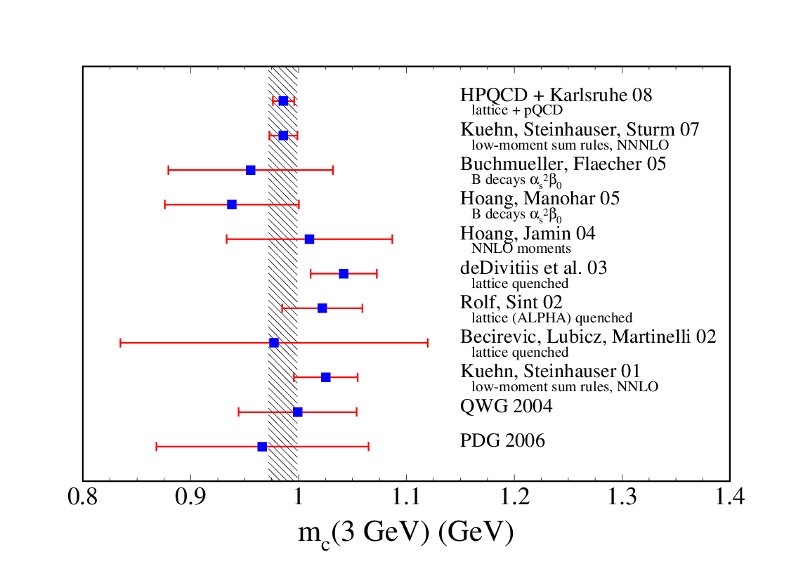 |
In Fig. 3 we compare the results of Section 2 and Section 3 with various other recent determinations. One observes a good agreement, however, our results are by far the most precise ones, as can be seen by the grey band.
Up to this point we have presented results for the charm quark mass evaluated at the scale GeV. In general, the comparison of results from various analyses are performed for the scale-invariant mass, (see, e.g., Ref. [1]). Note, however, that the scale is quite low and the numerical value of is relatively big. Thus, it would be more appropriate to perform the comparison at a higher scale like GeV. Let us nevertheless present the scale-invariant charm quark mass. From GeV one obtains
| (8) |
Acknowledgments
I would like to thank Konstantin Chetyrkin, Hans Kühn, Peter Lepage, Christian Sturm and the HPQCD lattice group for a fruitful and pleasant collaboration. This work was supported by the DFG through SFB/TR 9.
References
- [1] W. M. Yao et al. [Particle Data Group], J. Phys. G 33 (2006) 1.
- [2] V. A. Novikov, L. B. Okun, M. A. Shifman, A. I. Vainshtein, M. B. Voloshin and V. I. Zakharov, Phys. Rept. 41 (1978) 1.
- [3] J. H. Kühn and M. Steinhauser, Nucl. Phys. B 619 (2001) 588 [Erratum-ibid. B 640 (2002) 415] [arXiv:hep-ph/0109084].
- [4] J. H. Kühn, M. Steinhauser and C. Sturm, Nucl. Phys. B 778 (2007) 192 [arXiv:hep-ph/0702103].
- [5] I. Allison et al., in Lattice arXiv:0805.2999 [hep-lat].
- [6] J. Z. Bai et al. [BES Collaboration], Phys. Rev. Lett. 88 (2002) 101802 [arXiv:hep-ex/0102003].
- [7] M. Ablikim et al. [BES Collaboration], arXiv:hep-ex/0612054.
- [8] R. V. Harlander and M. Steinhauser, Comput. Phys. Commun. 153 (2003) 244 [arXiv:hep-ph/0212294].
- [9] A. E. Blinov et al. [MD-1 Collaboration], Z. Phys. C 70 (1996) 31.
- [10] R. Ammar et al. [CLEO Collaboration], Phys. Rev. D 57 (1998) 1350 [arXiv:hep-ex/9707018].
- [11] K. G. Chetyrkin, J. H. Kühn and M. Steinhauser, Phys. Lett. B 371 (1996) 93 [arXiv:hep-ph/9511430].
- [12] K. G. Chetyrkin, J. H. Kühn and M. Steinhauser, Nucl. Phys. B 482 (1996) 213 [arXiv:hep-ph/9606230].
- [13] K. G. Chetyrkin, J. H. Kühn and M. Steinhauser, Nucl. Phys. B 505 (1997) 40 [arXiv:hep-ph/9705254].
- [14] R. Boughezal, M. Czakon and T. Schutzmeier, Nucl. Phys. Proc. Suppl. 160 (2006) 160 [arXiv:hep-ph/0607141].
- [15] A. Maier, P. Maierhöfer and P. Marquard, Nucl. Phys. B 797 (2008) 218 [arXiv:0711.2636 [hep-ph]].
- [16] K. G. Chetyrkin, J. H. Kühn and C. Sturm, Eur. Phys. J. C 48 (2006) 107 [arXiv:hep-ph/0604234].
- [17] R. Boughezal, M. Czakon and T. Schutzmeier, Phys. Rev. D 74 (2006) 074006 [arXiv:hep-ph/0605023].
- [18] A. Maier, P. Maierhöfer and P. Marquard, arXiv:0806.3405 [hep-ph].
- [19] C. Sturm, arXiv:0805.3358 [hep-ph].
- [20] E. Follana et al. [HPQCD Collaboration and UKQCD Collaboration], Phys. Rev. D 75 (2007) 054502 [arXiv:hep-lat/0610092].
- [21] E. Follana, C. T. H. Davies, G. P. Lepage and J. Shigemitsu [HPQCD Collaboration and UKQCD Collaboration], Phys. Rev. Lett. 100 (2008) 062002 [arXiv:0706.1726 [hep-lat]].
- [22] A. Maier, P. Maierhöfer and P. Marquard, in preparation.
- [23] K. G. Chetyrkin, J. H. Kühn and M. Steinhauser, Comput. Phys. Commun. 133 (2000) 43 [arXiv:hep-ph/0004189].
- [24] P. A. Baikov, K. G. Chetyrkin and J. H. Kühn, arXiv:0801.1821 [hep-ph].
- [25] J.H. Kühn, TTP08-28, SFB/CPP-08-48, these proceedings.