Casimir Energy of a BEC:
From Moderate Interactions to the Ideal Gas
Abstract
Considering the Casimir effect due to phononic excitations of a weakly interacting dilute BEC, we derive a re-normalized expression for the zero temperature Casimir energy of a BEC confined to a parallel plate geometry with periodic boundary conditions. Our expression is formally equivalent to the free energy of a bosonic field at finite temperature, with a nontrivial density of modes that we compute analytically. As a function of the interaction strength, smoothly describes the transition from the weakly interacting Bogoliubov regime to the non-interacting ideal BEC. For the weakly interacting case, reduces to leading order to the Casimir energy due to zero-point fluctuations of massless phonon modes. In the limit of an ideal Bose gas, our result correctly describes the Casimir energy going to zero.
pacs
67.10.Fj, 03.75.Hh, 42.50.Lc1 Introduction
The Casimir effect is a consequence of the distorted vacuum fluctuation spectrum of quantized fields in bounded domains or spaces with non-trivial topologies [1, 2]. In Casimir’s original calculation, the system under consideration is the electromagnetic vacuum [3]. Imposing Dirichlet boundary conditions along one spatial direction by confining the system between two (idealized) parallel plates causes a change in the (infinite) vacuum energy-density. The variation of the vacuum energy-density with respect to the plate separation is called Casimir pressure, and, after renormalization, yields a finite expression for an attractive interaction energy per unit area between the plates. The electromagnetic Casimir force, caused by quantum fluctuations of the electromagnetic vacuum, is varying as with the plate separation and the speed of light . It has been measured in a number of experiments using various experimental settings [4, sec. 6]. The comparison between quantum vacuum experiments like these and the predictions of different theoretical models provides possibility to test fundamental physics (like higher dimensions or additional interactions), in much the same way as accelerator experiments in high-energy physics do at the other end of the energy scale [5, 6].
We consider here, instead of the electromagnetic vacuum, a weakly interacting Bose-Einstein-Condensate (BEC) at zero temperature, and expect, in a similar manner, the quantum fluctuations on top of the ground state of the BEC to give rise to observable Casimir forces: Within the Bogoliubov approximation, the excited states of a BEC can be treated as quasi-particles characterized by the dispersion relation
| (1.1) |
that behaves linear for small momenta, with the ‘sound velocity’ being inverse to the healing length . In (1.1), the wave-number characterizes the transition between the linear (phonon) and the quadratic (free-particle) regimes [7]. is also related to the -wave scattering length of the atoms and to the BEC density via . For small momenta, the quasi-particles (phonons) propagate in the same way as the massless electromagnetic field, except for the propagation velocity being different. Hence, the zero temperature quantum fluctuations in a spatially confined BEC can be expected to result in an observable Casimir force.
Different scenarios for Casimir forces in BECs have been analyzed by previous work: for the parallel plate geometry, an asymptotic expansion of the Casimir force has been calculated in [8], the small expansion parameter being the ratio between healing length and plate separation. In the leading order, it reproduces exactly the same behavior as in the electromagnetic vacuum. The next order corrections scale with the ratio . Replacing the perfectly reflecting plates by impurities embedded in a quantum liquid, Casimir forces between these impurities have been calculated in [9, 10] as a function of the impurity-liquid coupling. If the impurities are realized by atoms which, in a certain internal state, interact with the atoms of the quantum liquid through -wave scattering, the Casimir interaction should be detectable as a shift of spectral lines that depends on the distance between the impurities [10]. In the limit of an infinitely strong impurity-liquid coupling, the result for the (one-dimensional) parallel plate scenario was recovered [9]; for a weak coupling, however, the interaction between the impurities vanishes exponentially with the impurity separation on a scale set by the healing length. For the ideal (i.e. non-interacting) Bose gas, it was found that there is no Casimir force at all between impurities of arbitrary interaction strength, including the idealized parallel plate scenario [9, appendix C]. This is consistent with the quite general method of [11], which is mapping (polynomial) dispersion relations to Casimir forces in the parallel plate geometry: this method shows that media with quadratic dispersion relations, and hence the ideal Bose gas, do not give rise to any zero-temperature Casimir forces. A non-vanishing Casimir force in the ideal Bose gas can arise due to thermal fluctuations, as calculated in [12, 13]. All these forces are small but finite observable quantities, which—if experimentally confirmed—would provide direct evidence of the quantum fluctuations in weakly interacting BECs.
The system under consideration in the present article is a homogeneous, weakly-interacting dilute BEC at zero temperature, confined to a parallel plate geometry with periodic boundary conditions in one of the three spatial dimensions. The condition of diluteness can be formulated as , where is the -wave scattering length and is the density, being the total particle number and the volume of the gas. The quantity is usually called the gas parameter. The perturbative calculation of typical properties of such a BEC, like the ground state energy or the depletion of the condensate, is then essentially an expansion in the gas parameter [7].
For this system, we will give a re-normalized expression for the Casimir energy-density per unit area. Our expression has the form of an integral over a ‘density of modes’ times the Bose distribution function:
| (1.2) |
where has a simple analytic form (see (3.11)), and correctly describes the vanishing of the Casimir force in the limit of the interaction strength going to zero. The possibility to express the zero temperature Casimir energy in the above form, resembling the density of states of a bosonic system at finite temperature, is connected to a topological analogy between our parallel plate scenario and finite temperature field theory: In the parallel plate geometry, one spatial coordinate of the field is subject to periodic boundary conditions, while in finite temperature field theory, the imaginary time coordinate is subject to a similar periodicity condition. This analogy has been pointed out some time ago in [14]; it does not carry over, however, to Casimir calculations for non-linear dispersion relations. The periodic boundary conditions for the BEC have mainly been chosen because they make the relation to the finite temperature case particularly evident. In experiments, periodic boundary conditions can be realized in toroidal traps, but they also appear in optical lattices. If the boundaries are taken as real physical plates, the perfect mirror scenario (i.e. Dirichlet boundary conditions as discussed in [11, 15, 12]) is closer to an experimentally realizable situation. When Dirichlet boundary conditions are imposed on the fluctuations on top of the BEC ground state, the expansion of for moderate interaction shows in the leading term again the same behaviour as a massless scalar field propagating at the speed of sound , but with a different numerical prefactor.
The article is organized as follows: In section 2, we briefly recall some well-known perturbative expressions for the free energy, chemical potential and ground state energy of a dilute, weakly interacting BEC at zero temperature. Working from the formula for the free energy, we derive in section 3 the expression for the Casimir energy. In the limit , the function reproduces the power-series expression for the Casimir energy derived in [8], as is shown in section 3.1. In section 3.2, we relate the above mentioned analogy to the finite temperature case in some detail, as this topic does not seem to get overly much attention in the recent literature. Finally, section 3.3 deals with the behavior of the function in the limit of the effective coupling constant between the particles going to zero. Here, our expression correctly describes the vanishing of the Casimir force. We comment on the failure of the large-distance expansion to describe the non-interacting Bose gas. The case of Dirichlet boundary conditions is briefly discussed in the Appendix.
2 Free energy in a weakly interacting, dilute BEC at
In the one-loop approximation, the (unrenormalized) free energy density of a weakly interacting BEC at (in three spatial dimensions) is given by
| (2.1) |
with the mean-field and one-loop contributions [16]:
| (2.2) | |||||
| (2.3) |
Here and in the following, we work in units where . In the above expression, is the chemical potential (which, in section 3.1, will be connected to the speed of sound in the medium), and is the effective coupling constant that can, for low energy collisions in a dilute medium, be identified with the -wave scattering length : . The term represents the one-loop counter-term needed to render finite. If the integral in (2.3) is regularized with a momentum cut-off in the ultraviolet, the linear, cubic and quintic UV-divergences in can be absorbed by re-normalizing , and the vacuum energy respectively. If dimensional regularization is used in (2.3), no counter-term is needed at this level of perturbation theory.
After renormalization, the chemical potential can be obtained from (2.1) by inverting
| (2.4) |
which yields
| (2.5) |
Reinserting into (2.1) will then reproduce the classical result for the leading quantum corrections to the ground state energy density of a hard-sphere Bose gas, which was first derived by Lee, Huang and Yang in [17]:
| (2.6) |
3 The Casimir contribution as an integral over a density-function
Now, in order to describe a BEC between a pair of parallel plates separated by a finite distance (with periodic boundary conditions), we have to quantize the momentum component perpendicular to the plates:
| (3.1) |
Correspondingly, the momentum integration perpendicular to the plates is replaced by a discrete sum:
| (3.2) |
The area of the plates is taken to be with , so the system now inhabits the volume . The mean field contribution (see (2.2)) depends only trivially on the new boundary conditions, with the volume entering through in (2.5).
The Casimir energy of the BEC is related to the free energy at the one-loop level. We are interested in its change per unit area that is due to the introduction of the boundary conditions:
| (3.3) |
where the first term gives the (one-loop contribution to) the free energy in a homogeneous system. After applying the substitutions (3.1) and (3.2) to (2.3), we are left with the following expression for , now describing the leading quantum corrections to the free energy of a BEC confined between parallel plates:
| (3.4) |
where we have used the abbreviations
| (3.5) |
with and . The summation over can be converted into two integrals by using the Abel-Plana formula in the form (see [18])
| (3.6) |
Application of (3.6) splits (3.4) into the two terms written in (3.3), as the –term cancels out. The first term, , is divergent, but of the same form as the one-loop free energy (2.3) itself. Hence, it can be re-normalized as described above.
The term in (3.3), an energy per area, describes the effects induced by restricting the periodicity in one spatial dimension to be much smaller than the remaining ones, i.e., confining the system to a volume with one ‘short’ side . is convergent for any finite , strictly negative, and goes to zero for :
| (3.7) |
The integration domain is sketched in figure 1(a) (the shaded regions).

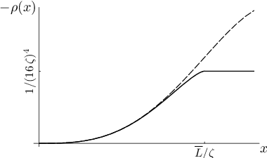
Fig. 1(a): The upper curve shows the function from (3.5), the lower one is . The two shaded regions make up the total area of integration in (3.7).
Fig. 1(b): The exact ‘density of states’ function from (3.11) (solid line) and its small-argument expansion (3.12)) (broken line).
This domain as well as the form of the integrand in (3.7) are due to the branch-points of the integrand in (3.4): In order to stay clear of the branch-cuts, we have evaluated the last term in the Abel-Plana formula (3.6) along an integration contour slightly to the right of the imaginary axis. Inserting the function given by (3.4),
| (3.8) |
the numerator in the last term of (3.6) evaluates to
| (3.9) |
being zero everywhere else along the contour of integration (see [1, sec. 2.2]). By changing the order of integration in (3.7), the -integral can be performed, and we find the expression (1.2) for the Casimir energy:
| (3.10) |
In the form of (3.10), is expressed as an integral over a ‘density of states’ (DOS) for a bosonic system, as setting the integration variable will reproduce the Boltzmann factor in the denominator.
The ‘mode density’ is obtained by integrating separately over the lower triangular region in figure 1(a) (dark gray) and the ‘hyperbolic tail’ (light gray). In terms of the dimensionless variable , we have
| (3.11) |
Above , the function changes into a constant independent of (see the solid line in figure 1(b)). The Casimir energy as a function of the normalized distance is shown in figure 2, obtained by numerically integrating (3.10).
To provide a cross-check for the above results, we will in the following section show that the function reproduces the asymptotic expansion for the Casimir energy given in [8, 19], which is valid for small values of the parameter . In section 3.3 we then show that the formula for in (3.11) also yields correct results in the opposite limit of the ideal BEC, i.e. .

3.1 Expansion at large distance and moderate interactions
In this section, we will assume the plate separation to be much greater than the healing length of the BEC, i.e., the ratio can be treated as a small parameter. Note that this limit cannot describe a strongly interacting Bose gas in the proper sense, since this would lead to the break-down of the one-loop approximation at the basis of our approach.
As can be seen in figure 1(b), the kink in the function happens at the large value in our limit. In evaluating the Casimir energy with (3.10), large values of , and hence the behavior of after the kink, get exponentially suppressed by the denominator. Thus we can approximate the function by expanding its small- part as a power-series around :
| (3.12) |
The integrals in the expression (3.10) for the Casimir energy can be performed explicitly.11 1 We use the identities in terms of the Gamma- and Zeta-functions. Upon setting (the speed of sound in the medium), we recover the result derived in [8]:
| (3.13) |
The leading term is, as noted in [8, 15], equal to the Casimir energy (per unit area) of a massless scalar field with propagation velocity confined between two parallel plates with periodic boundary conditions [20]. Its presence is a manifestation of the Goldstone-theorem, the long wavelength part of the Bogoliubov spectrum representing the gap-less Goldstone modes [21]. The next-to-leading term in (3.13) is in [8] referred to as the Bogoliubov correction due to the non-linearity of the dispersion. Indeed, if we express the Bogoliubov dispersion relation (1.1) as a power series around and put the first few terms into the expression for the Casimir force derived in [11, eqn. (16)], the leading term in the same manner reproduces the result for the scalar field (in one dimension), followed by terms that are smaller in magnitude and of opposite sign. As can be seen in figure 2, the contribution of these corrections is getting smaller as the ratio between plate separation and healing length increases, leaving only the dominant scalar term depicted by the horizontal dashed line in figure 2.
3.2 A formal analogy to finite temperature systems
As already mentioned, our expression (3.10) for at formally resembles the DOS for a bosonic system at finite temperature. This can be understood by recalling that a finite temperature system can be described in imaginary time, combined with periodic boundary conditions with period . The same topology is realized in the parallel plate system at , when one spatial dimension is subject to periodic boundary conditions with period ([14], see also [22]).
Let us briefly re-phrase the argument of [14] within our notation. The canonical partition function for a system at temperature in spatial dimensions is usually expressed as the path integral
| (3.14) |
where is the Lagrangian (a scalar functional of the field ), and the field is constrained in such a way that . If we take , the path-integral in (3.14) can, after Fourier expansion of the field, be evaluated to yield [23, 24]
| (3.15) |
Here, with are the Matsubara-frequencies due to the periodicity condition in (3.14), and with the continuous parameter is the dispersion relation of the massless scalar field. Note the similarity to (3.1), where we had periodic boundary conditions not in imaginary time but in one spatial dimension.
The sum over in (3.15) is usually evaluated by multiplying with a factor , which has poles of residue 1 at , and then integrating over a contour in the complex -plane which includes all the poles [24, sec. 3.4]. This technique is actually the same that is used in [18] to prove the Abel-Plana formula (3.6). The well known result is
| (3.16) |
where we have already subtracted the zero-point fluctuations. After integrating by parts and employing the integral-identity from the footnote on page 1, we obtain ( is the volume of the unit sphere in dimensions)
| (3.17) |
Note that, upon setting , the above expression has the same form as in (3.10), with being proportional to . Now, let the system inhabit a volume . With we get for the free energy per unit area
| (3.18) |
Tentatively exchanging with in (3.18) will reproduce the Casimir energy for a massless scalar field, i.e. the first term in (3.13) [14]:
| (3.19) |
So, we have seen that the zero temperature Casimir energy of a massless scalar field confined between two parallel plates can be obtained by a simple exchange of variables, once we know the thermal contribution to the free energy density of that field. Unfortunately, this simple mapping does not carry over to fields characterized by nonlinear dispersion relations: The temperature dependent part of the free energy for a BEC is (in the Bogoliubov approximation) still given by (3.16) with the dispersion now being [16]. But a simple interchange of with in (3.16) will no longer yield , because the discretized Matsubara frequencies (that become a discretized momentum) always enter in (3.15) in the same way as a spatial momentum component enters in a linear dispersion relation. It thus seems very difficult to mimic the fully nonlinear behavior of the dispersion relation.
3.3 The non-interacting limit
The transition from the weakly interacting BEC (here described at the one-loop level only) to the ideal BEC should be accomplished by letting the effective coupling (see section 2) go to zero, corresponding to . The Casimir energy is expected to vanish in this limit, as shown in [9, 11].
The series expansion (3.12) was constructed for , which is a physically reasonable assumption for finite L and a weak but finite interaction. But with the effective coupling strength , the chemical potential in (2.5) will vanish, too, and the healing length will diverge. As is kept finite, the non-interacting BEC is hence described by the limit , which is the opposite to the case considered in section 3.1. The asymptotic form of (3.12) for the mode density —as well as the Casimir energy in (3.13)—diverges in the limit of zero interaction strength. Our calculation of the exact mode density suggests that this divergence is due to a branch point in the complex -plane that moves towards and makes the power series expansion behind (3.13) break down. We show here that the exact mode density (3.11) leads to a Casimir energy that smoothly vanishes with the interaction strength (see figure 2).
To examine the asymptotic behavior of for , we again start from (3.10) and (3.11), separately treating the behavior of to the left and the right of the kink at :
| (3.20) | |||||
| (3.21) |
As the upper limit of the integration in is going to zero, we can replace by the first term in the expansion of (3.12), and Taylor-expand the denominator about . After integrating over this expansion, will yield terms of . Integrating , from the lower border of the integral we get a contribution
| (3.22) |
Altogether, we find for the behavior of in the non-interacting limit
| (3.23) |
Note that the leading order for at fixed goes like . Conversely, at fixed , a logarithmic divergence remains for . The logarithmic term changes sign for and, for large values of , the above expression diverges, just as the expansion (3.13) does for small values of (see figure 2). Hence, (3.23) and (3.13) provide two asymptotic expansions to for opposite limits, while the exact formula is given by (3.10) integrated over (3.11).
4 Summary
Starting from the free energy in a weakly-interacting dilute BEC, we derived a re-normalized expression for the ‘phononic’ Casimir energy of the BEC confined at zero temperature to a parallel plate geometry with periodic boundary conditions. Our formula for the Casimir energy (per unit plate area), (3.10), has the form of an integral over a density function times the Bose distribution. The function is given by a rather simple analytic expression in (3.11). In section 3.1, we provided a cross-check for our result by showing that a series expansion of in the parameter reproduces the asymptotic series for the Casimir energy derived in [8]. There, the Euler-MacLaurin formula was used to extract the long wavelength behavior out of the UV-divergent sum over all Bogoliubov modes satisfying the boundary conditions. This approach fails to reproduce the non-interacting limit.
As pointed out in [15, 8], the Casimir energy of the weakly interacting BEC is, due to the linear dispersion of its low lying excitations, in the leading order determined by a term analogous to the Casimir energy of a massless scalar field propagating with vacuum velocity . Our result displays this behavior in the regime of the weakly interacting BEC where the plate separation is much larger than the healing length, as can be seen in figure 2. In addition, for with kept finite (the non-interacting limit), our result (3.11) correctly describes the Casimir energy going to zero and displays the Casimir energy as a smoothly varying function of the interaction strength in the intermediate range. The subtleties of the asymptotic expansions illustrate the rich physical content behind the nonlinear dispersion relation of the Bogoliubov vacuum.
Appendix: Dirichlet boundary-conditions
Here we discuss how our results for the Casimir energy get modified with Dirichlet boundary conditions instead of periodic ones: taking the wavenumbers in (3.1) as with running from to infinity, application of the Abel-Plana formula generates an additional divergent surface-term in (3.3):
| (1.1) |
(The same term with opposite sign will appear for von Neumann boundary conditions, similar to [13] where the ideal gas at finite temperature is considered.) As does not depend on , it does not affect the Casimir energy. Our main formula for , (3.10), is modified by an overall factor , while in the mode density (see (3.11)) the distance argument picks up an additional factor of two:
| (1.2) |
The asymptotic expansion for large plate separation and moderate interactions, as derived in section 3.1, now yields (compare with (3.13)):
| (1.3) |
Again, the leading term is equal to the known result for the Casimir energy of a massless scalar field with propagation velocity confined between two parallel ideal mirrors (see [15, eqn. (38)]). For the non-interacting limit, as treated in section 3.3, we get the asymptotic expression (compare with (3.23))
| (1.4) |
This goes to zero as for periodic boundary conditions, with slightly different numerical factors.
The divergent surface energy (1.1) does not fit into the renormalization scheme for the bulk part of the free energy as described after (2.3). For a full treatment of the free energy of a BEC between perfect mirrors, it is not sufficient to change only the wavenumbers in the Bogoliubov excitations, because both the ground-state wave function and the excitations have to be zero on the boundaries. A detailed analysis will be reported elsewhere.
References
References
- [1] Mostepanenko V M and Trunov N N. The Casimir Effect and its Applications. Clarendon Press, Oxford, 1997.
- [2] Milton K A. The Casimir Effect: Physical Manifestations of Zero - Point Energy. World Scientific, 2001.
- [3] Casimir H B G. On the attraction between two perfectly conducting plates. Proc. Kon. Nederl. Akad. Wetensch., 51:793, 1948.
- [4] Bordag M, Mohideen U, and Mostepanenko V M. New developments in the Casimir effect. Physics Reports, 353:1, 2001.
- [5] Gies H. External fields as a probe for fundamental physics. J. Phys. A: Math. Gen., 41(16):164039, 2008.
- [6] R S Decca, E Fischbach, G L Klimchitskaya, D E Krause, D López, and V M Mostepanenko. Improved tests of extra-dimensional physics and thermal quantum field theory from new Casimir force measurements. Phys. Rev.D, 68(11):116003, 2003.
- [7] Pitaevskii L and Stringari S. Bose - Einstein Condensation. International Series of Monographs on Physics, 116. Clarendon Press, Oxford, 2003.
- [8] Edery A. Casimir forces in Bose - Einstein condensates: finite-size effects in three-dimensional rectangular cavities. Journal of Statistical Mechanics: Theory and Experiment, 2006(06):P06007, 2006.
- [9] Recati A, Fuchs J N, Peca C S, and Zwerger W. Casimir forces between defects in one-dimensional quantum liquids. Phys. Rev.A, 72(2):023616, 2005.
- [10] A Klein and M Fleischhauer. Interaction of impurity atoms in Bose-Einstein condensates. Phys. Rev.A, 71(3):033605, 2005.
- [11] Bachmann S and Kempf A. On the Casimir effect with general dispersion relations. J. Phys. A: Math. Gen., 41(16):164021, 2008.
- [12] Biswas S. Bose - Einstein condensation and the Casimir effect for an ideal bose gas confined between two slabs. J. Phys. A: Math. Gen., 40(33):9969, 2007.
- [13] Martin P A and Zagrebnov V A. The Casimir effect for the Bose-gas in slabs. Europhys. Lett., 73(1):15, 2006.
- [14] Toms D J. Casimir effect and topological mass. Phys. Rev.D, 21(4):928, 1980.
- [15] Edery A. Multidimensional cut-off technique, odd-dimensional Epstein zeta functions and Casimir energy of massless scalar fields. J. Phys. A: Math. Gen., 39(3):685, 2006.
- [16] Andersen J O. Theory of the weakly interacting Bose gas. Rev. Mod. Phys., 76(2):599, 2004.
- [17] Lee T D, Huang K, and Yang C N. Eigenvalues and eigenfunctions of a Bose system of hard spheres and its low-temperature properties. Phys. Rev., 106(6):1135, 1957.
- [18] Saharian A A. The generalized Abel-Plana formula with applications to Bessel functions and Casimir effect. arXiv:0708.1187 [hep-th], 2007.
- [19] Roberts D C and Pomeau Y. Casimir friction II: Casimir effect and drag in zero temperature superfluids. arXiv:cond-mat/0503757, 2005.
- [20] Svaiter N F and Svaiter B F. Casimir effect in a D-dimensional flat space-time and the cut-off method. J. Math. Phys., 32(1):175, 1991.
- [21] Hugenholtz N M and Pines D. Ground-state energy and excitation spectrum of a system of interacting bosons. Phys. Rev., 116(3):489, 1959.
- [22] Hawking S W. Zeta function regularization of path integrals in curved spacetime. Comm. Math. Phys., 55(2):133, 1977.
- [23] Bernard C W. Feynman rules for gauge theories at finite temperature. Phys. Rev.D, 9(12):3312, 1974.
- [24] Kapusta J I and Gale C. Finite-Temperature Field Theory. Cambridge Monographs on Mathematical Physics. Cambridge University Press, second edition, 2006.