Distortion of Wigner molecules : pair function approach
Abstract
We considered a two dimensional three electron quantum dot in a magnetic field in the Wigner limit. A unitary coordinate transformation decouples the Hamiltonian (with Coulomb interaction between the electrons included) into a sum of three independent pair Hamiltonians. The eigen-solutions of the pair Hamiltonian provide a spectrum of pair states. Each pair state defines the distance of the two electrons involved in this state. In the ground state for given pair angular momentum , this distance increases with increasing . The pair states have to be occupied under consideration of the Pauli exclusion principle, which differs from that for one-electron states and depends on the total spin and the total orbital angular momentum (sum over all pair angular momenta). We have shown that the three electrons in the ground state of the Wigner molecule form an equilateral triangle (as might be expected) only, if the state is a quartet () and the orbital angular momentum is a magic quantum number ( integer). Otherwise the triangle in the ground state is isosceles. For one of the sides is longer and for one of the sides is shorter than the other two.
pacs
73.21.La , 73.63.Kv Quantum dots
73.20.Qt Electron solids
31.30.Gs Jahn-Teller effect
I Introduction
Quantum dots are artificial atoms or molecules, where the electron number, the scalar potential and the magnetic field are tunable and can provide favorable conditions for all kinds of fascinating effects (for recent reviews see [1, 2, 3]). One effect is the formation of Wigner molecules (WMs). In [4] it has been considered and quantitatively described in the simplest system, the two electron dot, using the exact analytical solutions for this system [4]. In the present paper, another effect, namely a Jahn-Teller-like distortion of the WM, is analyzed. Again analytical solutions for the simplest system, where this effect can occur (the three electron dot), proved useful.
From the very beginning
we should be aware of the fact, that
Wigner localization
in circular symmetric systems
cannot be identified using
the electron density .
Because the Hamiltonian commutes with the total angular momentum operator,
the electron density can always be chosen circular symmetric
[5] and exhibits only a radial shell structure.
Non-circular solutions are an indication of degeneracy,
but not of Wigner localization.
The fact that the electrons keep more or less
fixed distances from each other due to
a strong electron-electron correlation
can be observed in
the pair correlation function
or the two-particle density matrix
or in spin resolved versions thereof.
For few electron dots both quantities are equivalent in exhibiting
the existence of Wigner molecules.
(In [4] the pair correlation function
in conjunction with the density
was used for describing the effect
instead of the
nowadays favored two-particle density matrix ).
A useful and illustrative notion of a WM in a circular symmetric confinement is a rotating and vibrating finite electron lattice [6, 7, 8, 9]. Due to this picture, a three-electron WM in a circular environment would form a equilateral triangle. In the present paper, however, we have shown that this is only the case in the classical limit where the distances between the electrons are so large that the exponentially decaying overlap between the localized wave functions of the individual electrons do not matter, but the long range Coulomb interaction is still effective. Shorter distances between the electrons and consequently overlap between the localized electron wave functions may lead to a distortion. Whether a distortion occurs depends on the angular momentum. This distortion of the seemingly natural equilateral symmetry is reminiscent of the Jahn-Teller effect, although in the present case the displaced objects are not atoms, but localized single electrons. (For a recent book on the Jahn-Teller effect including a lot of references see e.g. [16].) As shown below, the ground state of the WM for three electrons is isosceles including the equilateral as a special case. Excited states can be completely non-symmetric.
Meanwhile there are a couple of papers [10, 11, 12, 13, 15] which are focused on the case of three electrons. More work, which includes three electrons as a special case, can be found in recent reviews [1, 2]. The issue of the deformation of the WM without magnetic field has been discussed in [15] by investigating the two-particle density matrix using wave functions from exact diagonalization in an oscillator eigenfunction basis. The author found that with increasing coupling parameter (, ) there is a level crossing at , where the ground state switches from the to the state. He developed the following qualitative picture. In the quartet state (ground state for large ), the WM forms a equidistant triangle for all , whereas in the doublet state (ground state for small ) the spatial distribution is less trivial. Here, for infinite the electrons occupy the edges of an equidistant triangle. With decreasing the triangle is increasingly deformed into a isosceles one. This picture is a special case of the theory presented here. The purpose of the present paper is to extend the considerations to finite and to present a simple quantitative model.
II Decoupling into three pair problems
First, we want to review that part of the decoupling of the three-electron Hamiltonian into three pair Hamiltonians [13], which is vital for the general understanding of the current paper. A numerical check of the validity of this decoupling procedure for the three-electron problem in a three-dimensional confinement without magnetic field can be found in [17]. Unlike in [13], in the present paper we did not take advantage of the fact that for certain external field strength and quantum numbers there are analytical solutions of the pair equation, but instead we solved the radial pair equation (one-dimensional eigenvalue problem) numerically, whenever a concrete solution is required. The basic results, however, can be understood without having concrete numerical wave functions, but using only the Pauli principle.
The Hamiltonian for three electrons in a homogeneous magnetic field with the vector potential and a harmonic scalar confinement (oscillator frequency ) reads
| (1) |
This is in atomic units . For a model, where is replaced by an effective electron mass and by the effective (screened) charge , our results are in effective atomic units () defined by . Energies in our figures, which are generally given in units of or or a combination thereof, are therefore independent of the background parameters. In order to avoid the dependence of the results on any material dependent parameters, the Zeeman term with , is omitted. Besides, the Zeeman term has no influence on the focus of this paper, namely the spatial distribution of the electrons for given quantum numbers. It only shifts the energies and determines, what the quantum numbers of ground state are.
Now, we apply a unitary transformation from the original position vectors to new ones
| (2) |
where and . From the inverse transformation we obtain
| (3) | |||
where is the center of mass (c.m.) in the new coordinates, which agrees with the c.m. in the original coordinates . We do not use the Jacobi transformation (see also Appendix C), which separates the c.m. coordinate from the relative coordinates and which breaks the symmetry between the new quasi-particles. Instead, our transformation retains the symmetry and the c.m. is not an independent variable. Because any unitary transformation leaves the kinetic energy and the harmonic external potential invariant, the Hamiltonian in the new coordinates reads
| (4) |
While being still exact, (4) is not completely decoupled because contains all coordinates. In the Wigner limit, however, where the uncertainty of the c.m. vector is small compared with the mean electron- electron distance, we can neglect in the denominator of the interaction term in (4). As shown in the Appendices A and B, the quantitative errors introduced by this approximation are small and do not invalidate any of the qualitative conclusions of the present paper. Then, the Hamiltonian in zero order in
| (5) |
decouples into a sum of three independent pair Hamiltonians, which can be rewritten as
| (6) |
Here, is an effective confinement frequency, is the cyclotron frequency, and is the orbital angular momentum operator. This suggests the definition of a pair equation
| (7) |
with the normalization condition . The subscript comprises all quantum numbers. The pairs are essentially quasi-particles.
In polar coordinates we can make the following ansatz for the pair functions
| (8) |
where is an eigenvalue of and therefore the angular momentum of a pair. Inserting (6) and (8) into (7) provides the radial pair equation
| (9) |
with the effective pair potential
| (10) |
and the definition
| (11) |
The normalization condition reads . Fig.1 shows for two typical effective confinement frequencies . Observe that for has a minimum at non-zero only for .

Because of the decoupling in zero order, the total eigenvalues and orbital eigenfunctions of read
| (12) | |||||
| (13) |
The total energy is a sum of pair energies and the total orbital eigenfunction is a product of pair functions. In the original coordinates, the orbital eigenfunctions read
| (14) |
where, for the sake of obtaining simpler formulae, we introduced the following shorthand notation .
In order to avoid a basic misunderstanding, we want to stress that our independent-pair picture does not imply a division of all electrons into pairs, where each electron belongs exactly to one pair, as familiar from geminal approaches in Quantum Chemistry (see recent reviews in [14]) and which works only for even electron number. Instead, the total WF (14) is a product of two-electron (pair) functions, where each electron is involved in pairs with any of the other electrons. In [13] it has been shown that the high field limit of our wavefunction (WF) for agrees with the Laughlin WF for three electrons [10].
Now we want to discuss in an illustrative way, how the total WF (14) reflects the basic property of WMs, namely the strong e-e-correlation. Let’s consider the limit first. The radial part of the pair functions shows a peak at a certain coordinate value around the minimum of (see Fig.6), which we call the pair length and which will be calculated in Sect. 4. This means that the probability density of pair is peaked in -space whenever equals the pair length. Considering the special cyclic structure of the total WF (13) we can conclude: The probability density has peaks, if the three electrons form a triangle with sides equaling the three pair length. The angular orientation of this triangle is arbitrary, and its translational location is defined by . This triangle is blurred by the finite width of the peak in .
Although our theory is aimed at the strong correlation limit, we want to point out that also the weak correlation limit can be described by product wave functions in the new coordinates. (This will also be demonstrated in the next Section by investigating the numerical solutions of the pair equation in this limit.) The reason for the decoupling of the Hamiltonian (4), however, is quite different. Whereas in the strong correlation limit decoupling occurs because can be neglected versus , this is not the case for weak correlation. In the weak correlation limit, however, the whole e-e-interaction term can be neglected versus the kinetic energy. This leads to decoupling as well. Describing non-interacting electrons by products of WF in the new coordinates rather than simply by one-electron functions is just a complicated (but equivalent) way of describing the same system. This ambiguity is a consequence of the fact that (after neglecting the e-e-interaction) our Hamiltonian is invariant under any unitary transformation of the coordinates.
Because the pair functions are eigenfunctions of the orbital angular momentum operator in -space with eigenvalues , the total orbital eigenfunctions (13) are eigenfunctions of the total orbital angular momentum in -space with eigenvalues . Because the transformation back to the -space is unitary, (14) has the same eigenvalues like (13). Moreover, through (8) and (14), is linked to the parity of the total wave function. Even (odd) means even (odd) parity, i.e. symmetry (antisymmetry) with respect to inversion of all coordinate vectors.
III Pair energies and electron localization
The pair energies in our pair approach
are of the same central importance for the electronic structure of the system
as the one-particle energies in
independent particle systems.
The major qualitative difference between both approaches
lies in the occupation (Pauli principle) of the energy levels, which
has been investigated in Ref.[13].
Figs.2-4 show
the dependence of the ground state energies of the pair levels on the
orbital angular momentum of the pairs for fixed external field.
Fig.2 applies to the limiting case
of vanishing magnetic field.
In the limit
the pair levels converge to the one-electron levels for
non-interacting electrons (Fock-Darwin levels)
| (15) |
where the radial quantum number is the degree of excitation for given angular momentum . This can be seen in the radial pair equation (9,10): For large the state is compressed into the region of small , where the centrifugal term () is much larger than the e-e-interaction term () and the latter can be neglected. Without the e-e-interaction term the pair equation agrees with the one-electron Schrödinger equation.


Fig.3 shows the complementary case of vanishing
confinement. In the limit of strong magnetic fields,
these pair levels approach the ground states (for given )
of the Fock-Darwin
levels (15).
The analytical verification of this statement is evident in
eqs. (9,10).
It is also clear intuitively, because the strong magnetic field
out-plays the effect of the
Coulomb interaction.
A case with a fixed finite confinement ,
which is of the order of magnitude of quantum dots in GaAs
(in effective atomic units) is shown in Fig.4.
The angular momentum with minimum pair energy is now non-zero.


Fig.5 provides the angular momemtum of the lowest pair energy for given magnetic field and parabolic scalar confinement. The lines separate the regions with adjacent . In the upper left part of the plot and and in the lower right part converges successively to . In between only the lines separating the 10 lowest are shown. Although only a limited region of the parameter space is shown, the general features are obvious: All phase boundaries in the log-log-plot are well represented by parallel straight lines . Consequently, the boundaries in a linear plot are power functions where is universal and the factor depends on the boundary in question.
Fig.6 shows how
electron localization can be visualized in our approach.
Localization means that (the radial part of) the pair function ,
which describes the electron-
electron distance, is peaked at a finite x.
There are two reasons for localization:
a) for small (and small or vanishing ) the
electrons are pushed away from each other by
the (last) interaction term in (10).
On the other hand,
b) for large (and small )
the modulus of the angular momentum of the ground state is large
(see Fig.5).
In this case the separation of the electrons is caused by
the (first) centrifugal term in (10).
This mechanism does not work for vanishing because
then the angular momentum is ill defined. It does not work for
vanishing electron- electron interaction either.
Therefore, electron-electron interaction alone can localize the electrons
without the assistance of the magnetic field,
but the magnetic field alone cannot do the job.
As seen in Fig.6, the strongest localization is gained
for small (=0.01) and large (or at least medium) .
On the other hand, a medium (=1)
cannot achieve anything if
is of comparable size.
(The curve for =1, =0.01 agrees almost
completely with the curve for =1, =1.)
In this case we need a very
strong magnetic field (=100) for localizing the electrons.
A quantitative measure for localization is the mean square deviation
of from the expectation value .
The results read in the same order as shown in Fig.6: 0.0749, 0.00155, 0.1987, 0.2017, 0.00717.
IV Pair length and distortion of the Wigner molecule


As seen in Fig.7, the pair length define
the distortion of the Wigner molecule.
The pair length, or mean electron-electron distance,
can be obtained from the following quantities:
(i) the minimum position of the effective pair potential
(ii) the maximum position of the radial pair function
(iii) the average electron distance
| (16) |
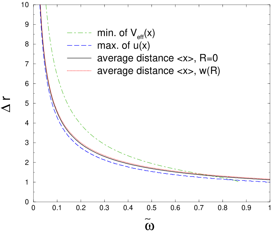
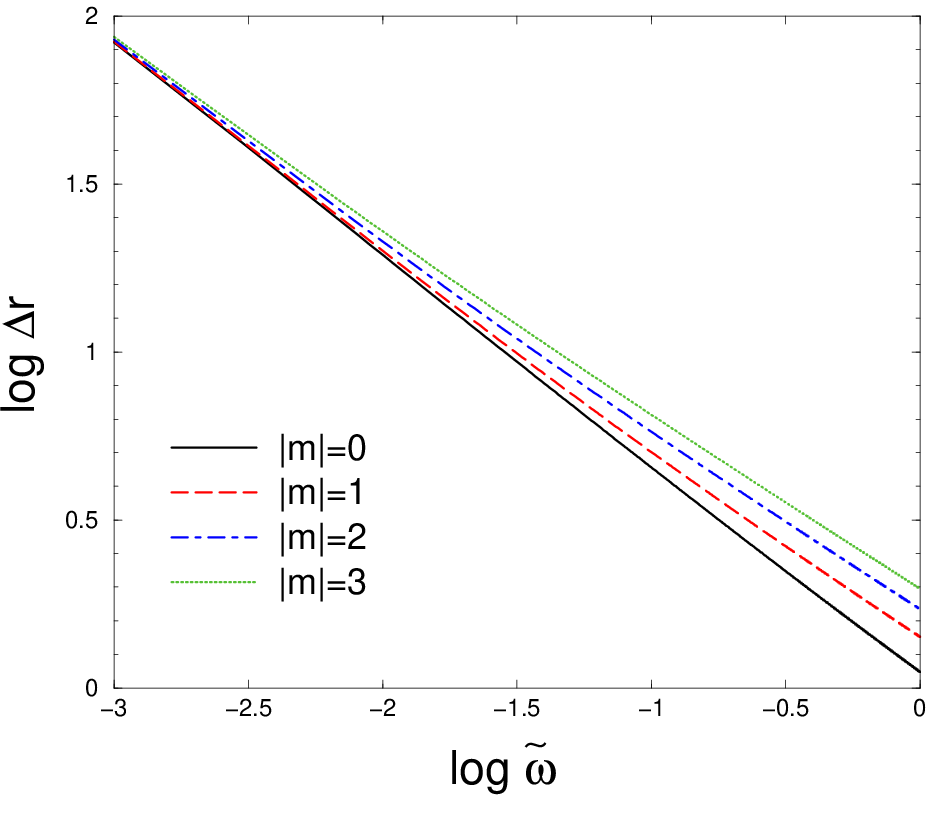
The real electron- electron distance is obtained from the above defined values by multiplication with as seen from (3). Definition (iii) agreed with (ii) if the radial pair function was symmetric with respect to the maximum, and (ii) agreed with (i) if it was -function like. In our curves discussed below, the radial wave functions of the ground state for the corresponding have been used throughout. Observe that for and the first definition breaks down completely, because has no minimum at non-zero (see also Fig.1). Fig.8 compares these definitions for . As to the agreement of the first and simplest definition with the two more sophisticated ones one has to consider, that a discrepancy of this size occurs only for , where the centrifugal potential in 2D is negative. The difference is much less for . Fig.9 shows the dependence of the pair length on the orbital angular momentum . Apart from getting an idea about the order of magnitude of the dependence, we notice that the pair length is the larger the larger is. (Observe that and depend only on the modulus of .) This follows directly from the fact, that the centrifugal potential in (10), which grows with growing , pushes the electrons within a pair away from each other. This effect can also be understood on the basis of classical mechanics. From the almost linear behavior in the log-log-scale we conclude, that the function of versus is roughly a power law.
For ground states,
the qualitative features of the distortion
may be grouped into three cases. In accordance with
Fig.s 2-4
we assume for the lowest pair state .
(a) If all three pairs are identical, i.e. ,
the triagle is equilateral. This case can occur only
in quartet states (parallel spins) and these
total orbital angular momenta are called ’magic’.
(b) The thick (black) lines in Fig.10 describe the
angular distortion of a WM composed of two pairs with and
one pair with .
Qualitatively, all pictures for two pairs with angular momentum
and one with , i.e. with , agree.
Then the WM spans a triangle where two sides are equal and one side is longer
than the other two,
because for .
The Pauli principle for pair states [13] demands that
this case can occur as in quartet (non-magic angular momentum)
as well as in doublet states.
(c) Fig.10 also shows the case for
two pairs with and
one pair with .
All WMs with two pairs with and
one pair with
providing look similar.
One side of the triangle is shorter than the other two equal sides
because and because this case can happen only for
.
The Pauli principle imposes the same restrictions
to the quantum numbers as in case (b).

It is clear that the distortion has to vanish in the limit , because in this limit the electrons behave like classical particles and their localized wave functions do not overlap. The distortion, however, is a quantum mechanical effect.
As can bee seen from the Pauli principle and the minimization of the total energy, in ground states the three pairs are never all different from each other. This does not apply to excited states where all three angular momenta can be different leading to a completely non-symmetric WM. The results of our theory for excited states have to be considered with some caution, however, because its applicability to excited states (in particular c.m. excitations) has not yet been investigated thoroughly. But this is not the topic of this paper.
V Summary
Using a simple unitary coordinate transformation and the Pauli principle, we have shown that a three-electron Wigner molecule in a quantum dot and a magnetic field can show a Jahn-Teller-like distortion. The qualitative fact of distortion can be shown analytically without any computations, but for a quantitative estimate we have to solve a one-dimensional eigenvalue problem (radial pair equation) numerically. In the ground states the Wigner molecule is either equilateral or isosceles, whereas excited states include completely non-symmetric geometries as well. If the state is a quartet () and the orbital angular momentum is a magic quantum number ( integer), the triangle is equilateral. In the doublet state () and for one of the sides is longer, and for one of the sides is shorter than the other two.
VI Appendix
VI.1 Estimate of the ratio x/R
For the ratio x/R, which is the relevant parameter for the decoupling in (4), can be estimated easily. The definition of the new coordinate in (3) reads
| (17) |
where we dropped the indexes and denote the electron distance by . An idea of the e-e-distance can be obtained from the classical e-e-distance in the ground state which is . The width of the c.m. probability distribution can be deduced from the exactly known c.m. wave function (see below) providing
Formula (17) with provides for the modulus
| (18) |
Because in the Wigner limit , we conclude and for the small decoupling parameter .
VI.2 Validity of the approximation X=R=0
Here we want to estimate the error due to the neglect of
in
i) the e-e-interaction term
in the transformed Hamiltonian (4)
ii) the pair length considered in Sect.4.
In a previous paper [13] the e-e-interaction term
was expanded in a multi-pole series (for )
and the correction terms were considered in
perturbation theory.
The problem with this approach is that the resulting series converges
slowly.
Additionally, it provides only the total energy in a simple way.
Therefore, we adopted here a different approach.
Because the probability distribution
of the c.m. is known exactly from Kohn’s theorem
(see Appendix C)
we averaged the corresponding quantities containing
with as weight function.
(For the estimates in this Appendix we adopted
for the angular momentum of the c.m. system .)
We replaced the e-e-interaction
potential
| (19) |
by the averaged potential
| (20) |
This virtually means using a smoothed e-e-potential (see Fig.11). Unlike perturbation theory, this approach does not destroy the independent-pair picture. Putting can also be viewed as using a -function-like c.m. distribution as found in the ground state of classical mechanics.
Despite the fact that the averaged e-e-potential in Fig.11 deviates or small strongly from the curve for , the change in the radial part of the pair function is very small. This comes from the fact that the probability density is small for those , where the averaged e-e-potential is changed by averaging. For the two curves for and are hardly distinguishable. The maximum shift in the pair energies due to averaging shown in Fig.12 is only about 1%.


Now we are considering the pair length. The relation between electron distances , the new coordinates and the c.m. vector is given in (3). Denoting for a chosen pair by omitting the index at , we have
| (21) |
Under the assumption of statistical independence, the probability density follows from the known probability densities
| (22) |
and
| (23) |
using
| (24) |
For the definition of the pair length we use the expectation value of the e-e-distance
| (25) |
Using (24), rescaling and after changing one of the integration variables we obtain
| (26) |
with the weight function
| (27) |
For -function-like c.m. distribution (corresponding to the approximation ) we have and the result from (26) agrees with the result from (16). Fig.13 shows that calculated with a finite distribution for deviates only for small from the result with . In this region, however, the radial pair function is small and the pair length for both approaches shown in Fig.8 deviate only marginally.

In the end we want to emphasize that the main conclusions of this paper, namely the qualitative statements about the distortion of the WM, are not influenced by averaging over . There are only small shifts in the pair energies and pair length. There is a hand-waving argument for this robustness against changes in the c.m. vector. It is connected to the Generalized Kohn theorem, which states that the c.m. coordinate decouples exactly from properly defined relative coordinates (see Appendix C). Therefore, no matter how large the width of the c.m. distribution is, it has no influence on the corresponding relative coordinates and on the internal structure of the WM. However, we have to consider that our relative coordinates are not completely decoupled from the c.m. vector, but are coupled weakly as indicated by the small shifts.
VI.3 Jacobi transformation
Applying the Jacobi transformation (see e.g. [19])
| (28) |
to (1) decouples the c.m. vector from the relative coordinates
| (29) |
where is the total momentum and are the canonical momenta belonging to . The distance between the electrons and thus the internal structure of the WM depends only on the relative coordinates
| (30) | |||||
This means that there is no correlation between the c.m. vector and the structure of the WM. For the estimates in Appendix A we need only the c.m. Hamiltonian which reads (for arbitrary electron number )
| (31) |
The c.m. eigenvalues are independent of and agree with (15), but the eigenfunctions are homogeneously compressed by a factor of . The latter read in polar coordinates
| (32) |
with the radial part for the lowest state for given
| (33) |
With (32) and (33) the probability density for reads
| (34) |
Acknowledgement I thank H.Eschrig and M.Richter for discussions. This work was supported by the German Research Foundation (DFG) in the Priority Program SPP 1145.
References
- [1] P.A.Maksym et al.,J.Phys.: Condens. Matter 12, R299 (2000)
- [2] S.M.Reimann, M.Manninen, Rev.Mod.Phys. 74, 1283 (2002)
- [3] C.Yannouleas, U.Landman, Rep.Prog.Phys. 70, 2067 (2007)
- [4]
M.Taut, Phys. Rev. A48, 3561 (1993)
M. Taut, J. Phys. A27, 1045 (1994) and
J.Phys.A27, 4723 (1994) (erratum)
Additionally, in formula (8) the factor has to be replaced by , in formula (10) in the term containing a factor is missing, and on the r.h.s. of (19a) and (20a) must be replaced by . - [5] K.Hirose, N.S.Wingreen, Phys. Rev. B 59, 4604 (1999)
- [6] F.Bolton, U.Rössler, Superlattices Microstruct. 13, 139 (1993)
- [7] P.A.Maksym, Phys. Rev. B 53, 10871 (1996)
- [8] C.Yannouleas, U.Landman, Phys. Rev. B 66, 115315 (2002) and J. Phys.: Condens. Matter 14, L591 (2002)
- [9] C.Yannouleas, U.Landman, Phys. Rev. B 68, 35326 (2003)
- [10]
R.B.Laughlin, Phys. Rev. B 27, 3383 (1983);
R. B. Laughlin, in: The Quantum Hall Effect, Eds. R.E.Prange and S.M.Girvin, Springer Verlag, New York (1987). - [11] P.Hawrylak, D.Pfannkuche, Phys. Rev. Lett. 70, 485 (1993)
- [12] D.Pfannkuche, Aspects of Coulomb Interaction in Semiconductor Nanostuctures, habilitation thesis, University Karlsruhe (1998)
- [13]
M.Taut, J. Phys.: Condens. Matter 12, 3689 (2000)
erratum: In formula (73), has to be read as , and 4 lines before, in the definition of , has to be replaced by . - [14]
P.R.Surjan, Top. Curr. Chem. 203, 63 (1999);
V.A.Rossolov, J. Chem. Phys. 117, 5978 (2002) - [15]
S.A.Mikhailov, Phys. Rev. B 65, 115312 (2002)
comment: The qualitative picture for small developed in this paper cannot be correct. The author writes at page 115312, right column, second paragraph:
’at small the one spin-down electron occupies the center of the dot, while the two spin-up electrons rotate around the center’
This is obviously not consistent with the fact, that for vanishing coupling two electrons with opposite spins occupy the oscillator state (which is centered in the middle) and one electron is left for the state, which is localized on a ring. Therefore one should rather say:
’two electrons with opposite spin are located in the center, while one rotates around the center’.
Qualitatively, this revised picture agrees with the numerical and plots as the original one does. The picture for growing has to be revised accordingly.
S.A.Mikhailov, N.A.Savostianova; Phys. Rev. B 66, 33307 (2002) - [16] I.B.Bersuker, The Jahn-Teller effect, Cambridge University Press 2006
- [17]
M.Taut, K.Pernal, J.Cioslowski, and V.Staemmler,
J. Chem. Phys. 118, 4861 (2003) - [18] R.Pauncz, Spin Eigenfunctions, Plaenum Press, New York and London 1979
- [19] L.Jacak, P.Hawrylak, and A.Woijs, Quantum Dots, Sect.4.1, Springer-Verlag 1998