Detecting Chameleons: The Astronomical Polarization Produced by Chameleon-like Scalar Fields
Abstract
We show that a coupling between chameleon-like scalar fields and photons induces linear and circular polarization in the light from astrophysical sources. In this context chameleon-like scalar fields includes those of the Olive-Pospelov (OP) model, which describes a varying fine structure constant. We determine the form of this polarization numerically and give analytic expressions in two useful limits. By comparing the predicted signal with current observations we are able to improve the constraints on the chameleon-photon coupling and the coupling in the OP model by over two orders of magnitude. It is argued that, if observed, the distinctive form of the chameleon induced circular polarization would represent a smoking gun for the presence of a chameleon. We also report a tentative statistical detection of a chameleon-like scalar field from observations of starlight polarization in our galaxy.
pacs
04.50.Kd, 97.10.Ld, 14.80.Mz, 98.80.CqI Introduction
Extensions of the Standard Model of particle physics, such as string theory, introduce many new scalar fields which are not seen in the Standard Model. Such scalar fields are commonly invoked to explain the observed acceleration of the universe, as inflation [1] or dark energy [2] fields, or to cause variations in fundamental constants [3]. If new scalar fields do indeed exist in the Universe, it is important to understand the properties of the theoretical models that describe them, e.g. the interactions of the scalar fields with themselves and with matter, which may give rise to additional observable effects that could be tested and constrained by experiments.
In this article we consider the effect of scalar field theories with a self-interaction potential, , and couplings to matter and light on observations of the polarization of light from astrophysical sources. These scalar field theories are described by the action:
| (1) | |||||
where the are the matter actions for the matter fields , and the functions and determine the couplings of the scalar field, , to the matter species, , and to the photon field respectively. A scalar field with such couplings to matter fields might be expected to give rise to fifth force effects or violations of the weak equivalence principle. In this article we are specifically interested in a scalar field, , which is light in relatively low density regions such as galaxies, galaxy clusters and the inter-galactic medium. More precisely, in these regions we require the mass, , of small perturbations about the background value of the scalar field, , to satisfy . Hence, any force mediated by would have a range . Additionally we require that coupling between photons and in these regions is relatively strong:
Therefore even if the coupling to matter is much weaker than the coupling to photons, since roughly of the mass of nuclei is due to electromagnetic interactions the -mediated force between individual nuclei in these backgrounds will be at least times the strength of gravity on scales smaller than .
One might, at first glance, conclude that a scalar field theory with these properties is already strongly ruled out by laboratory constraints, e.g. [4, 5, 6, 7, 8, 9], on the strength of fifth forces. Specifically, measurements of the displacement of a micro-machined silicon cantilever using a fibre interferometer, reported in [9], require that a Yukawa-type fifth force with strength times that of gravity has a range with 95% confidence. This, however, does not rule out the models we wish to consider as neither the strength nor the range of the -mediated force are necessarily the same in the relatively high density environment of the laboratory as they are in the low density background of space.
In recent years, two classes of models have arisen that allow a scalar field that is strongly interacting in low density environments and yet is currently undetected in laboratory tests: the chameleon model, [10, 11], and the Olive-Pospelov (OP) model [12]. Both models are described in detail in the following Section. The mechanism by which these models avoid laboratory tests can be understood by extremizing Eq. (1) with respect to to give the following field equation:
| (2) |
where
| (3) |
and is the trace of the energy momentum tensor for matter:
For non-relativistic matter , where is the energy density of the matter. Both the chameleon and OP models play the scalar field potential, , off against the matter couplings, and , to make the vacuum expectation value (VEV), and hence the properties of the field, depend strongly on the local density of matter. For convenience we shall refer to such a scalar field as the chameleon or chameleon field, however our analysis applies equally well to both the chameleon and OP models. In this analysis we posit a universal coupling to the different matter species i.e. . Although it is not required by either model, we make this assumption because it simplifies the analysis whilst having little effect our conclusions. The best constraints on come from the requirement that corrections to particle physics are small, which limits [13].
A coupling between matter fields and the chameleon potentially causes violations of the weak equivalence principle (WEP) and other fifth force effects such as an effective alteration to Newton’s inverse square law. A coupling between photons and chameleons introduces additional observable phenomena for the chameleon field. If such a coupling has super-gravitational strength, it can result in a non-negligible conversion of photons to chameleons and vice versa. The detectable effects associated with this conversion are similar to those predicted for axion-like-particles (ALPs) which interact with light [13]. Mixing requires the interaction between two photons and one scalar particle, and so the effects of the mixing are most likely to be seen when a photon, or a scalar particle is passing through an external electromagnetic field. The chameleon-photon coupling induces both birefringence and dichroism [13, 14] in a coherent photon beam passing through an external magnetic field. These effects could be detected by laboratory searches, such as the polarization experiments PVLAS, Q&A, and BMV [15, 16, 17, 18], that are sensitive to new hypothetical particles with a small mass and coupling to photons. Such experiments can constrain the coupling in the chameleon model, indeed the otherwise anomalous detection of birefringence with a magnetic field by PVLAS [16], could, at least in principle, be explained by the presence of a chameleon field [14]. For the most widely studied class of potentials, the PVLAS data was found to rule out [14]. In the OP model the mass of the scalar field in the laboratory is too large to produce a detectable effect in these experiments.
If chameleons exist and couple to photons, then they could, as suggested in [19, 20], be trapped and slowly converted back into photons resulting in a long lived chameleonic afterglow. A number of experiments, most notably GammeV [21], are searching or aiming to search for this afterglow effect. The GammeV chameleon search recently announced its first results which, for models with in the interior of the experiment, ruled out [22]. Ultimately GammeV may be sensitive to [19], and an optimal sensitivity for afterglow searches of is feasible within the constraints of currently available technology [19]. Indeed for any of the effects associated with the coupling to photons to be large enough to be detected in the laboratory, either now or in the foreseeable future, one must have . Such laboratory constraints do not, however, apply to the OP models.
These laboratory experiments need to be performed in a very good approximation to a vacuum otherwise the chameleon becomes too heavy to have a noticeable effect. A complimentary approach to testing chameleon-photon couplings is to look for the effects of the coupling in observations of astronomical objects. The densities of interstellar space are typically very low and so the effects of the chameleon may be significant. Light from all astronomical objects travels a significant distance through magnetic fields in galaxies, galaxy clusters and possibly in the intergalactic medium, before reaching the earth. However astronomical magnetic fields are typically made up of large numbers of randomly oriented magnetic domains - a very different scenario to the well controlled constant magnetic fields of laboratory experiments. In contrast to laboratory tests, such astrophysical effects should be see in the OP as well as the chameleon models.
The coupling between photons and chameleons means that photon number is not conserved, however, as the flux of photons emitted by astronomical objects is difficult to determine, measurements of flux cannot be used to bound the parameters of the chameleon model. In the following sections we show how the coupling between photons and chameleons generates polarization in the light from astronomical objects. Therefore measurements of polarization can be used to constrain the parameters of the chameleon model because the intrinsic polarization of astronomical objects is often very well constrained. Astronomers are interested in measuring polarization because it can provide information both about the source of the radiation and about any magnetic fields present between the source and the earth. Very precise astronomical polarization measurements are therefore available, and can be used to constrain the chameleon model.
This article is organized as follows: in §II we introduce and provide further details of the two classes of model to which our analysis applies i.e the chameleon and OP models. The coupling of a chameleon-like-particle to photons, is essentially the same as that which is assumed for a scalar axion-like particle (ALP). There is a great deal of literature concerning constraints (both local and astrophysical) on ALPs. However, the density dependent mass of a chameleon field, allows chameleon theories to evade the tightest of these constraints. In §III, we review previous constraints on ALPs, and consider to what extent they do, or do not, apply to chameleon-like models. In §IV, we consider how the existence of a chameleon-like field alters the polarization of light from astrophysical objects as it passes through an astrophysical magnetic field, and derive the form of the induced polarization. In §V we discuss the observed and predicted properties of the different types of large scale astrophysical magnetic fields. In §VI, we apply the results of the previous sections, and use astrophysical polarization observations to constrain the chameleon to photon coupling. We find that such measurements place the tightest constraints yet on this coupling. Applying the analysis to starlight polarisation in our galaxy we find a tentative statistical detection of a chameleon-like scalar field. Finally we summarize our results in §VIII.
II The Models
II.1 Chameleon Model
In the chameleon model the coupling functions and in Eq. (1) are well approximated by linear functions of i.e. and ; for reasons of naturalness, if , is usually assumed. The strength of the matter coupling is determined by and , hence in the chameleon model the coupling strength does not depend explicitly on the VEV of . The model was originally proposed by Khoury and Weltman [10] with , which results in a gravitational strength coupling between matter and the chameleon field, . The ability of the chameleon with this coupling to behave as dark energy was discussed in [23]. The coupling to photons, , was not expressly considered in [10] although with the most pronounced new effect is a virtually undetectable density dependence in the fine structure constant. With a gravitational strength coupling to matter (and possibly also photons) the chameleon field could be detected by laboratory, satellite, solar system and astrophysical tests (e.g. structure formation [24]) of gravity. A potentially much wider phenomenology was opened up, when Mota and Shaw [11] showed that coupling between chameleon fields and matter could be many orders of magnitude stronger than gravity, , and yet still be compatible with all existing experimental data. The properties of such strongly coupled chameleon fields can probed using experiments designed to measure the Casimir force [11, 25]. In addition, with a strong coupling and , Brax et al. [13] noted that interactions between chameleons fields and photons would result in potentially detectable effects similar to those predicted for axion-like-particles (ALPs) which interact with light.
It should be noted, that it is generally seen as ‘natural’, from the point of view of string theory, to have . This relation also arises in modified gravity theories (see e.g. Ref. [26] and references therein). It has also been suggested, however, that the chameleon field arises from the compactification of extra dimensions, [27]. In this case, there is no particular reason why the true Planck scale (i.e. that of the whole of space time including the extra-dimensions) should be the same as the effective 4-dimensional Planck scale defined by . Indeed having the true Planck scale much lower than has been suggested as a means of solving the Hierarchy problem (e.g. the ADD scenario [28]). In string-theory too, there is no particular reason why the string-scale should be the same as the effective four-dimensional Planck scale. It is also possible that the chameleon might arise as a result of new physics with an associated energy scale greater than the electroweak scale but much less than . Therefore in this article we consider as a free energy scale to be constrained by experiment. This said, to date, no one has managed to find such a chameleon theory (with either or otherwise) in the low-energy limit of a more fundamental high energy theory (e.g. supergravity).
The chameleon model evades the strong constraints imposed by local tests of gravity [10, 11] through non-linear self interactions of the field described by the potential , and hence the field may couple with super-gravitational strength. ‘Non-linear’ in this case means that is a strongly non-linear function of , and the mass of the scalar field, , therefore depends strongly on the VEV of . The VEV of in a given background is determined by the minimum of the effective potential, (3), and therefore the position of the minimum depends on and . is chosen so that is larger in high density regions than it is in low density regions. It is then possible to ensure that in a galaxy whereas in the laboratory . Assuming that and , the chameleon mechanism requires:
To provide some intuition for what we expect to be in a low density region such as a galaxy or galaxy cluster, we consider the most widely studied class of chameleon models where:
with , and . We note that this includes potentials with the form . is constrained by experiments to be at most a few orders of magnitude larger than the dark energy energy scale [11, 25]. When the chameleon is posited as an explanation for dark energy, it is therefore considered natural to take [10, 11]. The minimum of the effective potential occurs when where . The mass of the chameleon at this minimum is given by , so:
Assuming (i.e. the region which is not currently accessible to laboratory experiments), we have for all in a background, such as a galaxy or galaxy cluster, with .
II.2 Olive-Pospelov Model
The Olive-Pospelov (OP) model [12] was proposed as a way to allow particle masses and coupling ‘constants’ to depend on the local energy density of matter. The model could therefore provide an explanation for the difference between the value of the fine structure constant, , in the laboratory and that extrapolated from the spectra of 128 QSO absorption systems at redshifts by Webb et al. [29]: . There is now a great deal of tension between other potential theoretical explanations for this data see e.g. Refs. [3, 30], and the most recent local atomic clock constraints on any local time variation of [31, 32, 33]. In the OP model, is locally time-independent and hence these constraints are avoided.
The OP model could also describe a density dependent electron-proton mass ratio . Reinhold et al. [34] reported a indication of a variation in . They analysed the wavelengths of the spectra of two absorbers at and observed using the Very Large Telescope (VLT), finding . It was shown, however, in Ref. [35] that due to wavelength calibration errors in the spectrograph on the VLT identified in Ref. [36], the result of Reinhold et al. could no longer be trusted. The reanalysis performed by King et al. [35], in which data from an additional object at was also included, found , which is consistent with no change. Very recently Levshakov et al. [37] have reported evidence for a spatial variation in found by measuring ammonia emission lines in the Milky Way: .
All of these astronomical measurements of and , were made in regions where the average density of matter, is very low compared to the ambient density of matter in a laboratory. The background density for all of these measurements, , is similar to the average density of a galaxy or galaxy cluster i.e. . These measurements could therefore be an indication that some or all of the ‘constants’ of Nature depend on the ambient density of matter. The OP model realises just such a density dependent variation in a manner that does not conflict with local tests of gravity. In this model, the coupling functions, and , are chosen so that they are close to their minimum (which occurs at ):
For reasons of naturalness, one would expect [12]. In contrast to the chameleon model, the OP model does not require that the potential, , contain non-linear self interaction terms, and in the simplest model:
In a background with density , assuming , as is usually the case, and fixing the definition of by setting , the value of at the minimum of the effective potential, is given by:
| (4) |
In the laboratory environment, , and so . Additionally the effective matter coupling is small enough to evade experimental constraints. In low density regions such as galaxies , so . The change in between the laboratory and a low density region such as galaxy is given by:
To explain the Webb et al. value [29] of , one would require .
Olive and Pospelov [12] found that the current best constraints on are and . We define to be the mass of small perturbations in in a low density region (i.e. ), and let specify the range of the -mediated force in such a region. It was found in [12] that
For there to be measurable differences between the particle masses and coupling constants in the laboratory and in regions with , one must require:
In the low density regions where the effective coupling to the photon field for small perturbations in is:
It is clear then that a field with the required properties, and , is perfectly compatible with current experimental constraints.
We note that in [12], the value suggested for , which is compatible with all current constraints, is . Now:
so for , we have which corresponds roughly to .
III Constraints on Axion-Like-Particles
Axion-like-particles (ALPs) can either be scalar or pseudo-scalar fields which couple to the electromagnetic field strength. If it were not for the chameleon mechanism (i.e. the density-dependent mass) present in the chameleon and OP models, they would essentially describe a standard scalar ALP. There are tight constraints on the coupling, , of ALPs to photons. In the previous section, we discussed constraints from local experiments on chameleon-like particles, however such particles are also constrained by searches for ALPs. For a recent review of the astrophysical constraints on ALPs see Ref. [38] and reference therein. In all cases, these constraints only apply when the ALP mass, , lies within a certain range e.g . The mass of a chameleon-like particle is not, however, fixed and so applying these constraints to chameleon models is non-trivial. We must take great care to identify the ambient density of the region wherein the constraint on is required to derive the bound on .
The strongest astrophysical constraints in Ref. [38] come from axion production in the cores of stars. The application of the constraints of solar axion production to chameleon-like models has previously been studied in Ref. [13] and [39]. The Sun may be a powerful source of ALP flux, and the predicted effects of the loss of energy of the Sun through ALP emission allows one to constrain the coupling . It must be noted, that all solar ALP constraints require that the ALPs actually escape the sun. The strongest solar ALP constraints come from limits on the solar neutrino flux, and this gives:
Similar constraints result from the CERN Axion Solar Telescope (CAST) which attempts to directly detect solar axions. However it was shown in Ref. [13], that solar chameleon-like ALPs would generally bounce off, rather than enter the CAST instrument, and so the CAST constraints cannot be applied to chameleon models. Similar constraints are found from the life-time of Helium burning (HB) stars in globular clusters: . Solar axion constraints are derived from production of axions in the solar core by the Primakoff process. In this region the temperature is , and the typical density is . In the Helium burning stars, and . All of the constraints assume that . It was shown in Ref. [39], that all solar axion production bounds are evaded if in the solar core. Similarly, the Helium burning star constraints are effectively evaded if in their cores. For example, if one considers a chameleon potential like , where , one finds that with a matter coupling of , we have in the core regions of the HB stars, and in the solar core. With the different choice of potential, , one finds in the cores of Helium burning stars but in the Sun when . Thus the solar and HB star axion constraints on would apply to the latter potential with but be evaded by the former. If we took , then both potentials would evade these constraints. Thus in the chameleon model, whether or not these astrophysical constraints are relevant depends greatly on the properties of the potential, and in particularly how it determines the behaviour of the theory at high densities. In general, these properties cannot be inferred from the low-density behaviour of the theories. We are concerned only with the low density behaviour in this work.
At high densities, the scalar field in the OP model couples quadratically, rather than linearly (as an ALP would) to the QED term. In this way it avoids astrophysical constraints related to axion production in high density regions.
Recently, in Ref. [40], it was shown that polarization measurements of -ray bursts could be used to constrain axion production at the source of the burst. Whilst later in this article we will consider the potential constraints on chameleon-like fields from -ray burst polarization measurements, we will be interested in constraining any polarization that is induced by the chameleon as the light from the -ray burst passes through low-density magnetized regions of space (e.g. the interstellar and inter-galactic mediums). We will assume that axion production in the immediate vicinity of the -ray burst itself is negligible. In Ref. [40], it is assumed that, in the vicinity of a -ray burst, there is a magnetic field of strength over a distance of about . Given this, it is found that:
for . For larger values of :
It is noted that in the vicinity of the GRB, , corresponding to . The effective ‘energy density’ to which the chameleon field couples is not just but . Thus for the GRB, . Such a places one in the high-density region of the OP model, where the only couples to photons quadratically and hence no longer behaves as an axion. In chameleon theories, if where and (as is usually assumed), one finds that when
Thus the strongest constraint on from Ref. [40] does not apply here. If we take or then we predict or respectively for ; hence is allowed. Indeed, we find that the bound of Ref. [40], would allow all such chameleon models with .
It should also be noted, that axion-like chameleon production from the magnetic fields of neutron stars would also be greatly suppressed. For a neutron star , which corresponds to and hence a very heavy chameleon particle.
It is clear then that astrophysical ALP constraints coming from relatively high density regions do not apply to the OP model, and the extent to which they apply to a chameleon theory depends greatly on the precise choice of potential. For at least one popular choice of potential () one of the constraints noted above applies. Furthermore, because the chameleon field is very heavy in high density regions, we expect any initial chameleon flux from stars or objects to be greatly suppressed relative to that which one would expect for a standard ALP.
There has also been a great deal of work on conversion of photons to very light ALPs in relatively low density backgrounds (e.g. the interstellar medium). See, for example, Refs. [41, 42, 43, 44, 45, 46], and for a recent review see Ref. [47]. In relatively low density regions, chameleon-like particles behave essentially like standard axion-like-particles. Therefore much of the analysis presented in the aforementioned works is directly applicable. Only where a initial axion flux from, for example, a star or quasar has been assumed will the analysis differ. Many of these studies have focused on photon-axion conversion in the inter-galactic medium. Magnetic fields with strength are generally seen as plausible in the inter-galactic medium. It is suspected that such fields would be coherent over scales of about a megaparsec or so. We discuss this further in §V. For reasonable values of the electron number density, , in the inter-galactic medium, it is commonly found that or so [47].
Carlson and Garretson [44] specifically considered the effects of photon to ALP conversion induced by the magnetic field of our own galaxy. This discussion is directly relevant to our work. In their work they were only able to constrain , however they suggested a method that would allow couplings down to to be probed. In our work to use a different method to constrain down to . Ref. [44] is also interesting because it is noted that small scale fluctuations in the electron-density can lead to an enhancement of the photon to ALP conversion rate. In their work, the enhancement effect was estimated to be very large for visible light. We discuss this further in Appendix A, and note that the size of the enhancement effect found in Ref. [44] was in part due to, what is now, an old model for the electron-density fluctuations. Using the more recent NE2001 model [48], we show in Appendix A that the enhancement effect is expected to be no larger than in the local interstellar medium. Due to the complexities and additional uncertainties associated with the structure of electron-density fluctuations, particularly at parsec scales, which determine the magnitude of any enhancement, we have neglected the potential enhancement effect of Ref. [44] from our analysis. As we note in Appendix A, however, we do not expect this to greatly alter our conclusions. Similarly, the analysis of Ref. [46] is applicable to chameleon-like fields, however our analysis goes beyond what was presented there.
We also comment on Ref. [45]. Here a supercluster magnetic field with strength coherent over a scale of was assumed. Additionally an enhancement effect similar to that derived in Ref. [44] was employed. It must be noted that the magnitude of any enhancement effect depends greatly on both the magnitude and the spatial scale of the spectrum of electron-density fluctuations. The former is fairly well known for electrons in our galaxy, whereas the latter is less well known. In the context of electrons in a supercluster neither is well known. Additionally evidence for a field strength of coherent over was tentative at best at the time that Ref. [45], and a more recent analysis [49] suggests that if such a field does exist it is either weaker, , or only coherent over much smaller scales . Even if such a field does exist, it is also not clear precisely what distance along the line of sight the field extends. As such, the constraint: quoted in Ref. [45] relies on many assumptions, with at best only tentative observational support. Removing any one of these assumptions, would allow for much larger couplings. In this work, we are primarily concerned with constraints on photon to chameleon conversion in astrophysical regions where there is strong evidence for magnetic fields, and the properties of such magnetic fields are relatively well known. We also note in Appendix A that making the reasonable assumption or smaller (where the indicate a spatial average), any enhancement of the photon-chameleon conversion rate due to electron fluctuations is expected to be sub-leading order at optical (and higher) frequencies for cluster and super-cluster scale magnetic fields.
IV Chameleon Field Optics
In this section we consider how the presence of a chameleon field alters the properties of light propagating through one, or many, magnetic regions. Varying the action Eq. (1) with respect to both and gives Eq. (2) and
| (5) |
where is the background electromagnetic 4-current: . We consider propagation of light in an astrophysical background which contains a magnetic field of strength . The background value of is denoted . We write the perturbation in the photon field as and the perturbation in the chameleon field as . Ignoring terms that are and assuming that the proper frequency of the photons, , is large compared to the Hubble parameter, , we find that:
| (6) | |||||
| (7) | |||||
where and
and here is the background density of matter.
We assume that is small enough that we may make the approximation:
where is the chameleon mass. If the photons are moving through a plasma with electron number density , they will behave as if they had an effective mass squared , where is the plasma frequency; is the fine structure constant and is the electron mass.
IV.1 A Single Magnetic Domain
We define and to be the components of the photon field perpendicular and parallel to the magnetic field , and take the photon field to be propagating in the -direction. From Eq. (6) we have:
For such a system, it is well known that the probability of a photon, with frequency , converting to a chameleon particle (or vice versa) whilst travelling a distance through a region with a homogeneous magnetic field is:
| (8) |
where
| (9) | |||||
| (10) | |||||
| (11) |
and . Generally and so the last term in is dropped. Following [14, 19, 50], we find that, up to an overall phase factor, , and are transformed by passing through a homogeneous magnetic domain in the following way:
| , | (12) | ||||
| (13) | |||||
| (14) |
where and and
| (15) |
Since we must, in realistic situations, allow the light to be partially polarized (or even unpolarized), it is insufficient to consider simply the evolution of the photon, and , and chameleon amplitudes. We must instead represent the properties of the photon field by its Stokes vector. We therefore make the following definitions:
| (16) | |||||
The Stokes vector for the photon field is , where describes the amount of circular polarization (CP), and and describe the amount of linear polarization (LP). We also define the reduced Stokes vector: . The fraction of light which is polarized is:
and the fractional circular polarization is:
We also define . The fractional linear polarization is .
We normalise the photon and chameleon fluxes so that (this quantity is conserved), where . We also define . With these definitions we find that, on passing through a single homogeneous magnetic domain, the components of the Stokes vector transform as:
| (17) | |||||
| (18) | |||||
| (19) | |||||
Additionally, the , , and amplitudes transform as
| (20) | |||||
| (21) | |||||
| (22) | |||||
From these equations it is clear that the presence of a light scalar field coupling to photons can result in the production of polarization. This is because, when a chameleon (or another axion-like particle) is converted back into a photon, that photon is polarized perpendicular to the magnetic field. If we consider the simple case where initially there is no chameleon flux so that and , and we set , and initially then, using , it is clear that upon exiting the magnetic domain:
If the initial total and circular polarization fractions are and , their final values are
| (23) | |||
| (24) |
where and . It is therefore possible for both linearly and circularly polarized light to be produced. In a single magnetic domain, the production of the former is due to the conversion of photons into chameleons and then back into photons, and the latter is due to the birefringence of the medium which is induced by the presence of the chameleon field. If initially , then after passing through a single domain:
We also note that if there is no initial chameleon flux or polarization, , no CP can be produced in a single magnetic domain. As we shall see below, the same is not true if there are multiple magnetic domains.
IV.2 Multiple Magnetic Domains
In many realistic astrophysical settings, including the ones we will be primarily concerned with in subsequent sections, light passes through many magnetic domains on its way from a source to an observer. In each domain the angle, , describing the inclination of the background magnetic field to the direction of propagation is essentially random. Solving the full system of evolution equations for a large number of magnetic domains involves diagonalising an 8 by 8 matrix as well as evaluating multiple sums involving the random angle , and we have been unable to find a general analytic solution, however, it is straightforward to solve the system numerically. This said, approximate analytical solutions exist in a number of interesting and important limits. A full presentation of the equations that must be solved in this set-up, and their analytic solutions in these limits is provided in Appendix B. We present the results of that analysis below. We define to be the number of magnetic domains through which the light has passed, and in all cases assume that there is no initial chameleon flux.
For fixed and magnetic domain length , we define a critical frequency such that , and hence . When , is almost independent of frequency, however when , . We also define to be the critical wavelength and .
IV.2.1 Weak Mixing Limit
In a great many realistic situations we have and and, as we shall show, the frequency dependence of the production of linearly and circularly polarized light in this limit is qualitatively similar to that seen in general. In this limit we must have either and , or and , and so
In Appendix B we find that when an initially unpolarized light beam, with frequency , from a single source passes through domains (and requiring and ), the final polarization fraction, , and final fractional CP, , are essentially random variables and are described by the following distributions:
where at fixed , the are approximately independent identically distributed random variables and
When the are roughly independent of , but when there is a strong , and hence wavelength dependence. The above expressions describe the total and circular polarization fractions for a monochromatic light beam from a single source. If one has observations of many objects all at the same frequency the average value of , denoted , and r.m.s. average of , denoted , are more useful quantities for comparing with observations. For the distributions above
| (25) | |||||
| (26) |
where is now the average number of magnetic regions. When , and when , .
When some initial polarization is present ( and say, so that the initial linear polarization is ), we find a different behaviour: When (but keeping ) the average final polarization fractions, and are still given, to , by Eqs. (25) and (26) respectively. When we find instead that to :
| (27) |
and
| (28) | |||||
where this expression is only accurate to leading order in .
We shall see that for realistic astrophysical magnetic fields the critical wavelength generally corresponds to UV or X-ray light. As such most polarimetry measurements of astrophysical objects will have been made at wavelengths . For such wavelengths, the analytical solutions found in Appendix B show that the reduced Stokes parameters, , and , exhibit a strong and oscillatory frequency dependence. This behaviour is very important when one wishes to make comparisons with observations. Polarimeters always have some finite wavelength () resolution, . This is usually referred to as the spectral resolution. Thus a measurement of the reduced Stokes parameters at some wavelength , will actually measure an average of their values in the window . If one averages the reduced Stokes parameters over wavelength bins much larger than much of the information about a chameleonic contribution will be lost. Specifically if we assume and then, to , and where:
| (29) | |||||
| (30) | |||||
where for , and are independent identically distributed random variables. Thus, in this case, constraints on the parameters of the scalar field theory could only be derived by measuring both the total polarization fraction and the CP fraction. When , if the spectral resolution is too poor or the data is placed into too wide wavelength bins, the measured polarization fraction, , carries little or no information about the properties of . For optimal sensitivity to chameleonic effects, the spectral resolution of the polarimeter and the size of the wavelength bins must satisfy . We discuss in §IV.3 below how when the spectral resolution is sufficiently good, the strong wavelength dependence at wavelengths can be exploited to extract strong constraints on chameleon-like theories from observations of a single object.
IV.2.2 Maximal Mixing Regime
When , if the chameleon to photon coupling is strong enough and , i.e. if , maximal mixing will occur. In this limit the equations that must be solved simplify greatly. Further details of the calculations are given in Appendix B. The strong mixing limit is appropriate when , and . When there is little production of circular polarization, and so the main effect is the production of linear polarization. Additionally since at high frequencies we expect for astrophysical objects we set the initial circular polarization fraction to zero, and the final CP fraction, , remains .

We find that the final (linear) polarization fraction, , in this limit, does not explicitly depend on or any other properties of the chameleon field and that it is given by the following distribution:
| (31) | |||||
where and are independent uniform random variables: and . We note that when , does not depend on frequency. If we average over observations of many sources (each with and ) then we would measure the average polarization fraction . In the simplest case where we have:
and so
More generally
is a monotonically increasing function of and increases from to as goes from to . It is clear that in the strong mixing limit, the presence of a chameleon-like field coupling to the photon can induce a significant amount of linear polarization. We find that the following formula
| (32) | |||||
fits extremely well. We plot against the exact value of in FIG. 1. The solid line is the exact value and the dashed line shows . Also shown on this plot is the line . For , the average polarization after maximal chameleon mixing is larger than the intrinsic polarization , whereas for it is slightly less.
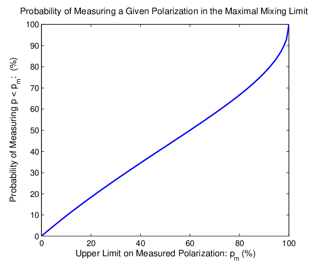
If one were to measure for a large number of astrophysical objects then at least one of the following must be true: or . When , the chameleon induced polarization is largely independent of frequency, and so the spectral resolution of the polarimeter is not as important as it is in the weak mixing regime. The probability of measuring the total linear polarization of a random object to be less than some , when and mixing is maximal (), is shown in FIG. 2; we have assumed no knowledge of the initial intrinsic polarization and hence marginalized over a uniform prior for it.
IV.2.3 General Behaviour
When, as is often the case, one excepts little or no intrinsic circular polarization of the light beam i.e. , we are able to combine the results presented in the previous two subsections to provide a fitting formula for the general form of the mean value of after the light beam has passed through magnetic domains. We find
where
In the maximal mixing limit . In the weak mixing limit, when , we have:
So if is small, we have , as required. If instead is larger, . This provides a very good fit to the simulated data in all cases.
IV.3 Optical Signatures of Chameleon Fields
We presented above the results of a mathematical analysis of how the presence of a light scalar field coupling to matter would alter the polarization properties of light passing through a magnetic field, the details of which can be found in Appendix B. By combining the results of this analysis with numerical simulations, we now detail the main physical signatures that a chameleon field would imprint on the polarization properties of light from astrophysical sources. Above we found that there were two main effects:
- •
the production of polarization,
- •
the production of circular polarization.
Each of these effects depends on frequency in a characteristic manner that is well illustrated by considering the weak mixing limit of §IV.2.1 above with no initial polarization (). In this limit but for all and . This requires ; is the maximum value of .


We consider the weak mixing limit, assuming that the polarimeter has wavelength resolution where and is the total path length of the light through the magnetic field. In this limit, when there is no initial polarization, both the induced degree of polarization: , and circular polarization are proportional to . FIG. 3 shows possible simulated forms for the rescaled total polarization degree, , linear polarization and CP for two different hypothetical objects, where for example in both cases. We can clearly see from this that production of linear polarization is greatest for and CP polarization production is peaked in the region . As expected, we can also see that both the induced linear and circular polarization degrees are highly frequency dependent for .

Assuming , averaging , and over many sources each at roughly the same distance, and hence with roughly the same , gives and . The forms of , and are shown in FIG. 4. We see that both quantities grow strongly when and that is peaked between and . The form of the averaged CP degree, , is very distinctive. The height of the peak, as well as the maximum value of are determined by , whereas the position of the peak and its width are fixed by and . If such a peak should be resolved, one would in principle be able to determine both , and the coherence length, , of the magnetic field regions. Measurements of circular polarization for could therefore provide a powerful tool with which to constrain chameleon theories; we discuss this further in §VII. Qualitatively similar behaviour is seen for the chameleonic induced polarizations in the more general case where can take any value and the intrinsic (i.e. non-chameleonic) polarization is not restricted to vanish. When is allowed, the chameleonic production of linear polarization is peaked for where:
| (33) |
CP production is in general peaked between and .
In practice, however, as we shall discuss further in §VI below, it is rare for current polarimeters to have ; although measurements do exist with . As well as requiring , to measure , and one must also have measurements of many sources where the light from each source is expected to have passed through roughly the same number of magnetic regions, each with roughly the same properties, as the light from any other source. This requirement introduces a fair amount of uncertainty and will ultimately limit ones ability to accurately constrain the averaged quantities. Another problem is that even when the intrinsic polarization is small (), if , the form of , and are highly dependent on . Unless one can measure or accurately predict the intrinsic polarization, this again limits ones ability to accurately constrain chameleon theories.
Many astrophysical polarization measurements are made at wavelengths where the chameleon induced contribution to the Stokes parameters exhibits a highly oscillatory wavelength dependence. When and provided or smaller, we can exploit this property to extract strong constraints about the properties of any chameleon-photon interaction from observations of a single object without any detailed prior knowledge of . We do this by defining a smoothing scale which is picked to be but smaller than the wavelength scale over which the intrinsic polarizations, , and , are expected to vary strongly. By removing the smoothing signal from the measured signal we should recover a superposition of any induced chameleonic signal and the noise. Assuming that the noise is either random or that it does not have a wavelength structure that mimics that of the induced chameleon signal we can extract constraints on . Further details of how can be constrained in this manner are given in Appendix C. Using this method, it is possible to extract strong constraints on using data from only a single source.
V Large Scale Astrophysical Magnetic Fields
The largest scale magnetic fields that are known to exist are those associated with galaxies and galaxy clusters. In both cases the mean field strength has been measured to be roughly a few micro Gauss. It is also thought likely that a weak, , magnetic field permeates the inter-galactic medium (IGM). We discuss the observed properties of first two fields as well as the hypothesised properties of the latter below. The electron density, , determines the plasma frequency, , which plays a critical rôle in determining the effective chameleon mass, , and hence also critical frequency, , above which polarization production is peaked. Therefore we also quote the observed or estimated values of for each of the three regions.
V.1 Galactic magnetic fields
Galactic magnetic fields, particularly those of our own galaxy, could produce detectable polarization effects if chameleon-like fields interact strongly enough with photons. Galactic magnetic fields have been observed to be a superposition of a regular magnetic field, , and a random magnetic field, (see [51] and references therein). The regular component of the magnetic field has a coherence length, i.e. about the scale of the galaxy [51]. The component of the regular part of the magnetic field along the line of sight to distant objects such as pulsars and extragalactic radio sources has been measured using Faraday rotation. These measurements are performed using electromagnetic waves whose frequency is well below . The interpretation of such measurements would therefore be largely unaltered by the presence of a chameleon field or similar light scalar field. The average regular magnetic field in own galaxy is locally (within about of the Sun): [52, 53], rising to about in the more central Norma arm [54]. The magnetic field is aligned with the disk of the galaxy, and is coherent out to a galactic radius of about , field reversals then occur at , and [51, 55].
The random magnetic field, , is often slightly larger than the regular magnetic field. The largest scale of the turbulent field was determined from pulsar rotation measures (RMs) as by Rand and Kulkarni [56], with a turbulent field strength about about . A similar study by Ohno and Shibata [57] found with a random field strength of . has also been estimated by the depolarization of light by turbulent fields at centimetre radio wavelengths, and by Faraday dispersion at decimetre radio wavelengths [55]. Both methods give results consistent with .
Recently Sun et al. [55] combined radio telescope and WMAP measurements of diffuse polarized radio emission from the Milky Way with Faraday rotation measurements to obtain an overall model of the Milky Way’s magnetic field. They found that on average G with field reversals occurring over kiloparsec scales, and G with . The average electron density was taken by Sun et al. to be . Generally light observed from objects within our own galaxy will have passed through regions of the regular magnetic field, but different coherent regions of the random magnetic field. Taking and G for the random magnetic field and we have:
| (34) |
and so
| (35) |
When and hence , Å. For an object in our galaxy at a distance we take . Therefore if, as is typical, we have .
Taking G for the regular magnetic field and we have:
| (36) |
and
| (37) |
so when , Å. We note that for .
In the weak mixing regime, i.e. when the chameleon induced polarization is small, we find that the total induced polarization is a sum of that which would be separately induced by the random and regular magnetic fields.
For the dark energy inspired chameleon model discussed in §II.1, we have in the galaxy, and hence , for all when .
V.2 Intracluster magnetic fields
In galaxy clusters electron densities of are typical, as are magnetic field strengths of a few , rising to tens of G at the centre of cooling core clusters. These magnetic fields are coherent over length scales of about [58]. Galaxy clusters typically extend over a length scale of . A light beam traversing a galaxy cluster would therefore pass through roughly magnetic regions.
In a study of data from 53 radio sources located in and behind Abell clusters and a control sample of 99 sources Kim et al. [59] found the mean core electron density of a cluster to be , where the radius of the core is , and found cluster magnetic field strengths of G with coherence length . A study of 18 radio sources close in angular position to the Coma Cluster by Kim et al. [60] found the following result for the strength of magnetic fields in the intracluster medium (ICM):
| (38) |
where is defined in terms of the Hubble parameter today: . A subsequent study, again of the Coma cluster, by Feretti et al. [61] found tangled magnetic fields with length scales of about , so . A study of 16 low redshift () “normal” galaxy clusters by Clarke, Kronberg and Böhringer [62] found that the ICM of these clusters was permeated by a slightly larger magnetic field:
Based on the studies of Kim et al. [59, 60], we take the follow representative values for the parameters which describe magnetic fields in the ICM:
We define to be the path length a given light beam traverses through a cluster, and take as a representative value . The number of magnetic regions, , is given by , and hence we take
With these values we have and
| (39) |
and
| (40) |
When , Å. We note that when .
In galaxy clusters, we have for the chameleon model introduced in §II.1 for all when .
V.3 Intergalactic magnetic fields
Although a number of different mechanisms have been suggested that would produce large scale magnetic fields in the intergalactic medium (IGM), at the present time very little is known about whether such fields actually exist, let alone their typical strengths. A coherent magnetic field on the current horizon scale would produce an anisotropic expansion. CMB and Faraday rotation constraints on such a scenario limit G [63, 64]. Faraday rotation also constrains smaller scale magnetic fields. For a coherence length one has G, and G for Mpc scale coherence lengths [64]. The CMB has also been shown to constrain fields with a coherence length between and to be G [65]. Motivated by the need to explain the origin of galactic magnetic fields it is thought that IGM magnetic fields with coherence lengths of a few Mpc are likely (see [66] and references therein). Most of the proposed theoretical mechanisms for generating such fields would, however, only produce them with strengths well below the current observational upper bounds [66]. These seed fields are then amplified by some dynamo mechanism during galaxy formation to the G galactic magnetic fields observed.
Typical electron densities in the IGM are giving and so
| (41) |
and
hence for and , we have Å. For the dark energy chameleon potentials discussed in §II.1, the mass of the chameleon due to the density of the IGM is i.e. for if and the chameleon couples only to baryons. If the chameleon couples to dark matter with equal strength then the same is true but only for .
VI Current Polarization Constraints on Chameleon-like Models
In this Section we review a number of astronomical polarization observations and deduce how they constrain the properties of any chameleon-like field.
We noted in §IV.2.1 that at wavelengths , any chameleon induced polarization signal is a highly oscillatory function of wavelength, with oscillation length . This is particularly important as many astrophysical polarization measurements are made at optical frequencies for which , and either the Stokes parameters are put into wavelength bins with width , or the spectral resolution of the polarimeter is so poor that it effectively averages over a range of wavelengths which is . In either situation, any signal of chameleon mixing will be washed out, and no constraints on the chameleon model are possible. If there is no initial polarization the polarization fraction depends on via and , these are all highly oscillatory functions of except when . We note that in some cases the spectral resolution of the polarimeter is good enough to resolve any chameleon induced polarization, but the published data only quotes the Stokes parameters in bins much wider than . In these cases, the published data cannot bound chameleon-like theories but constraints should follow from a reanalysis of the raw data. By way of an example, we have performed such a reanalysis for observations of three stars in our galaxy, however in general such a reanalysis is beyond the scope of this article, and is intended to form the basis of a future work.
VI.1 Starlight Polarization
Polarization is not usually produced by the thermal emission of stars. In [67] a statistical analysis of the largest available compilation of galactic starlight data [68] was performed. The data is statistically significant for sources out to distances of , and the average polarization of light from stars at such distances is .
This data, provided in the polarization catalogue [68], is in very wide wavelength bins that generally cover the whole range of optical frequencies, i.e. the bin width is Å. For comparison, the oscillation length, , in the galaxy for such stars is Å for both the random and regular components of the magnetic field. Thus and the data provided in [68] as well as the subsequent analysis of [67] does not provide useful constraints on chameleon-like theories.
Existing starlight polarization measurements can, however, constrain chameleon-like theories. UV polarization of starlight was measured for 121 objects by the Wisconsin Ultraviolet Photo-Polarimeter Experiment (WUPPE), which flew on the ASTRO-1 and ASTRO-2 NASA space shuttle missions, and had a nominal spectral resolution of Å[69]. The data from these observations is available from the Multimission Archive at STScI (MAST) [70]. A full reanalysis of the data for all 121 objects is beyond the scope of this work, however we have derived preliminary confidence limits on in the galaxy using data from three objects: HD2905, HD37903 and HD34078. These objects were picked as they all lie at distances between and , which is not so close that a chameleonic signal would be too small to detect, and not so far away that numerical calculations involved in extracting the confidence limits on are too time consuming. Other than that, the choice of objects is entirely arbitrary. A detailed account of the method and resulting confidence limits derived from the polarization measurements of these objects is given in Appendix C. Intriguingly, we found that the data from all three objects preferred a non-zero value of at a prima facie statistically significant level. This analysis shows that there is some structure in the polarization data which is consistent with the signal that we predict would be induced by a chameleon field. It would be premature, however, to claim this as an actual detection before a similar analysis has been conducted for more objects, and before a thorough analysis of all systematics which could be sources this signal has been undertaken. The most conservative, in the sense that they are the widest and are expected to be the most robust, confidence intervals were found using the bootstrap-t method (see Appendix C for further details). At 95% confidence we found, taking and Å:
| (42) | |||||
| (43) | |||||
| (44) |
If we assume that the same value of is appropriate for each object, by combining the polarization data for all three stars we find that the estimate of is approximately normally distributed with mean and variance ; . Hence we find the following approximate confidences
| (45) | |||
| (46) |
From this preliminary analysis, it therefore appears as if the polarization data of the three objects considered is consistent with a value of which deviates from by more than .
Although this analysis is only preliminary, it does appear as if there is a reasonably significant, and robust, statistical preference towards the existence of a chameleon-like field in the starlight polarization data of the three objects we have considered here. This is a highly surprising result, and as such it would be premature to claim it as a detection. Whilst it is well beyond the scope of this particular article, a thorough analysis of possible backgrounds and sources of systematic error which could mimic the signal from a chameleon field would have to be undertaken before any such claim could be made with true confidence. In particular, since all the data analysed comes from a single experiment (WUPPE) it possible that the ‘detection’ of a non-zero value for is actually due to effects intrinsic to the instrument. In order to quantify the magnitude of such instrumental effects it would be necessary to study similar data from other polarimeters. We have only considered three of the well over one hundred objects measured by WUPPE. When more objects have been analyzed it should be possible to better estimate the effect of systematic error in the determination of by considering the spread in the values of determined for each object. What we can say with confidence is that there is some structure in the polarization of three objects considered which is not consistent with either random error or that predicted to be induced by interstellar dust. Furthermore this structure exhibits non-trivial oscillatory frequency correlations which at least in part mimic that predicted by the chameleon model. At the present time we cannot rule out possible systematic effects having a relative magnitude of . The presence of such effects would raise both the extracted upper and lower bounds bounds on . Whilst this means that any non-zero lower bound on can only be seen as tentative at best, the upper bounds on should be robust. We therefore believe it to be better to see the data as providing the following 95% and 99.9% confidence upper bounds on :
| (47) | |||
| (48) |
We also consider observations of the UV polarization of two stars made with the Faint Object Spectrograph (FOS) of the Hubble Space Telescope (HST) and reported in Ref. [71]. In this case, we have only undertaken a preliminary analysis of the data, postponing a full reanalysis to a later work. Observations were made for Å Å, and the HST FOS has a nominal spectral resolution of Å in this range. The data published in Ref. [71] was binned to give ten data points in each frequency region they considered, although the precise width of the bins is not stated. The shortest wavelength region was Å. Assuming that each of the ten bins in this region had equal width, the bin width is Å. The two stars, HD7252 and HD161056, are respectively and from the earth. This gives an oscillation wavelength, , no smaller than Å and Å for the random and regular components of the galactic magnetic field respectively, when . A significant amount of a chameleonic signal should therefore survive the rebinning process in the Å wavelength grating; this may not be the case for the lower frequency gratings. In the Å grating, the polarization angle of HD7252 was found to be independent of frequency with a standard deviation of about degrees. It is noted in Ref. [71] however that the systematic uncertainty in the polarization angle could be degrees or so. This corresponds to the component of the reduce Stokes vector, say, that is perpendicular to the mean polarization detection in the region Å satisfying . Assuming in the galaxy and that (the precise value of does not greatly alter the resulting constraint) so that Å, and using the method outlined Appendix C.2, we find the following % and % confidence limits
These constraints are consistent with, but weaker than, those found from the WUPPE data.
VI.2 The Crab Nebula
The polarization of X-ray light from the Crab nebular was reported in [72]. The measured linear polarization fraction was at a frequency of and at a frequency of . This confirmed the hypothesis of synchrotron X-ray emission. The Crab nebula is at a distance of 2kpc from the solar system so photons from the Crab nebular pass through regular magnetic domains and random magnetic domains to reach the earth. When , we have Å; . Thus both measurements are in the region, where is almost independent of frequency. The spectral resolution of these measurements is Å.
The linear polarization fraction, is given by a probability distribution even if we are in the maximal mixing regime and so the amount of information one can extract from a single measurement is limited. We found that the average polarization fraction for a set of objects in the maximal mixing limit is . However, if initially, one would still expect to measure for a given object about of the time. Even the possibility of maximal mixing at X-ray frequencies cannot therefore be ruled out by the Crab Nebula data.
VI.3 Type Ia supernovae
In [74, 73] supernova polarimetry data published before 1996 was studied. The degree of polarization of light from type Ia supernovae was less than . In [75] high-quality spectro-polarimetry data was reported for SNIa 2001e1. It was found that the maximum linear polarization of the light from the supernovae was . The supernova was observed at frequencies and the spectral resolution of the polarimeter was Å. The Stokes parameters were later re-binned into Åbins. The supernova lies at a redshift of corresponding to a distance of roughly .
If, as light travels from the supernova to the earth, mixing with chameleons occurs mostly in the intergalactic medium (as opposed to in galaxies or clusters) then the PVLAS bound rules out maximal mixing. The critical frequency for weak mixing in the intergalactic medium is , where is the coherence length of the IGM magnetic field. Since we have ; Å. Hence SNIa 2001e1 was observed at frequencies . Any chameleon induced polarization fraction would therefore be a highly oscillatory function of the frequency. For this chameleon signal to survive the binning process and be detected one must ensure that the polarimeter’s spectral resolution and width of the wavelength bins satisfy Å. In this case Åand so the data can indeed be used to constrain chameleon-like theories. At the wavelengths observed, the chameleonic signal would look like random noise that grows with frequency. A full analysis of the raw data reported in [75] is beyond the scope of this work. However, a preliminary analysis of the scatter in the component of the Stokes vector perpendicular to the mean direction of polarization, , in the frequency range Å provides strong constraints. At five different epochs, it was found that was consistent with zero to within about . We take and extract approximate upper confidence limits on the chameleon to photon coupling using the method detailed in Appendix C.2. When in the IGM, and , we find the following % and % confidence limits
If the intergalactic magnetic field is sufficiently small (i.e. ) mixing between light from the supernova and chameleons will occur mostly in galaxies and galaxy clusters. SNIa 2001e1 is located in the nearly edge-on spiral galaxy NGC 1448, however the line of sight does not intersect with either the core or the disk of the host galaxy [75]. Additionally, at only away, light from SNIa 2001e1 does not pass through any significant intra-cluster magnetic fields. Our solar system currently lies close to the midpoint of the galactic plane, and models of the galactic magnetic field and electron density suggest that it has a scale height above the midpoint galactic plane of about a kiloparsec. At the very least then, light from SNIa2001 will have passed through roughly of the random galactic magnetic field. For the random galactic magnetic field we have Å, where when . Therefore Å, and a chameleon signal could be detected. Since , the chameleon induced polarization would look like random noise. Again a preliminary analysis of the data of [75], gives the follow 95% and 99% confidence limit, where we have assumed in the galaxy and that the coherence length of the random component of the galaxy magnetic field is so that Å:
VI.4 High Redshift Quasars
The optical and UV polarization of some high redshift quasars have been measured [76, 77] often using the HST FOS. Below frequencies the quasars have a polarization of about 1% but there is an interesting rise in the polarization above frequencies . At electron-Volt frequencies mixing between photons and chameleons is expected to be highly frequency dependent. The HST FOS has a nominal spectral resolution of Å, which is in principle good enough to resolve the expected chameleon signal if in galaxies or galaxy clusters. The data in [76, 77] is then rebinned with bin widths of Å. Extracting the most stringent constraints on chameleon theories would require a full reanalysis of original data. This is beyond the scope of this article. However, by analysing the data of Impey et al. [76] for object PG 1222+228 at as rebinned and presented in Ref. [77] we can extract useful constraints. Specifically, we focus on the spread of the Stokes parameter that is perpendicular to the mean polarization angle. The light from this QSO will have travelled at least . We assume that the coherence length of the random component of our galaxy’s magnetic field, , is . Making the conservative assumption that the total path length through our galaxy’s magnetic field is , when in the galaxy, we find the following 95% and 99% confidence limits:
We expect that a full reanalysis of the original data would raise this limit greatly as currently the bounds are considerably weakened by the relatively large size of the wavelength bins (compared to ).
If there is a sufficiently strong intergalactic magnetic field then this would also produce chameleon-photon mixing. We make the conservative assumption that IGM magnetic fields only go out as far as , so that the propagation distance through the IGM magnetic field is about . Assuming the IGM magnetic field is coherence over roughly megaparsec scales, we find the following confidence limits when in the IGM:
These constraints are particularly strong because the quasar is so far away, and as such the light from it travels through many different coherent regions, , of any IGM magnetic field. This counter balances the loss of information due to the relatively large width of the wavelength bins. A full reanalysis of the raw data would likely raise these bounds on .
VI.5 Gamma Ray Bursts
Measurements of linearly polarized gamma rays have been made for four GRBs and these are summarised in Table 1.
The last observation has been challenged [78]. GRBs are the only objects we consider that are believed to be highly polarized initially. Theory predicts the emission of highly linearly polarized light with due to synchrotron emission. This hypothesis was confirmed by observations of polarization in the GRB afterglow [82].
Mixing at gamma ray frequencies is maximal in all galaxies and clusters regions if : maximal in galaxies if and in the ICM if . If in the IGM, then maximal mixing would occur if ; however if in the IGM then this scenario is strongly ruled out by the bounds obtained above. If the mixing is maximal the mean observed linear polarization at high frequencies should be ; consistent with current GRB observations. It is not possible to make a more precise prediction than this without knowing more accurately the initial polarization of the GRB. A better understanding of the central engine of the GRB and better polarimetry for GRBs would allow strong constraints to be placed on the chameleon model. If future observations constrain maximal mixing in the chameleon model would be ruled out, and strong constraints on would follow. If is observed such a high degree of polarization cannot be explained by the synchrotron mechanism and a chameleonic explanation would be favoured.
If is very large the mixing between chameleons and light from GRBs would be weak. Then it becomes difficult to put bounds on the chameleon model both because of the limitations of polarimeters and, if there is no intergalactic magnetic field, the difficulty of estimating how many magnetic domains have been traversed.
VI.6 CMB Polarization
The upcoming Planck satellite will measure the polarization of the CMB to a high degree of accuracy. However it is extremely hard to estimate how many magnetic domains radiation from the CMB would have passed through, particularly as if there is an intergalactic magnetic field it is not known whether this field is primordial. Neglecting the intergalactic magnetic field it might be possible to use galaxy and cluster surveys to estimate how many magnetic domains the radiation had passed through. However because the frequency of CMB radiation is so low mixing with the chameleons will be weak and highly oscillatory and the amplitude of these oscillations is damped as . A weak and highly oscillatory chameleon signal would be very hard to detect.
VI.7 Summarised Constraints
The tightest constraints on the chameleon to matter coupling come from the WUPPE starlight polarization data, in the context of photon to chameleon conversion in the galaxy, and from HST FOS measurements of the polarization of high redshift quasars in the context of conversion in the intergalactic medium. Our preliminary analysis of starlight polarization data appears to provide a non-zero lower bound on , however for the purposes of this discussion we only consider the upper bounds on here. For the IGM we took the coherence length, , to be and for the galaxy we assumed, , however the precise values of these quantities do not greatly effect the upper bounds on . Taking these typical values for and for the strength of the random component of the galactic magnetic field, we find at confidence:
| (49) | |||||
| (50) |
At confidence we find similarly
| (51) | |||||
| (52) |
In both cases the upper constraint applies if in the galaxy and the lower one if in the IGM. Since is currently unmeasured, the strongest constraint on is comes from the starlight polarization measurements, the interpretation of which relies only on knowledge of the galactic magnetic field. If , however, then the constraints coming from high redshift quasars currently provide the tightest lower bounds on . In terms of chameleon theories, these constraints represent an improvement of almost 2.5 order of magnitude on the previous best lower bounds on coming from laboratory tests, specifically at confidence from the GammeV experiment [21].
GammeV and other similar laboratory tests do not constrain the OP model. Provided in the galaxy, and it was shown in §II.2 that this is expected to be the case, the starlight polarization constraint on the OP model translates to:
| (53) |
at confidence where is the fractional difference between in the laboratory and in a background such as the galaxy. For comparison, the previous best constraints were and . If as suggested by the analysis of Webb et al. [29], then this represents an improvement of two to three orders of magnitude. We note that if a subsequent analysis were to confirm the lower bound on found from starlight polarization measurements, then both these measurements and the Webb et al. value of could be explained by an OP model with
and ; .
VII Circular Polarization: A smoking gun?
The total polarization due to chameleon-photon mixing grows as the square of the frequency of the light until it reaches a critical frequency at which the mixing becomes maximal. It has not been possible to detect this frequency pattern in current linear polarization data. Objects whose initial polarization is well constrained have not been observed over a wide enough frequency range or to the required accuracy to see any such signal. Certain GRBs have been observed over a very large range of frequencies as they evolve, but because their initial linear polarization is not known accurately, and generally does not satisfy , it is difficult to search for a chameleon signal in this data.


The production of circular polarization by chameleon photon mixing has a much more interesting signature. One does not usually expect significant amounts of intrinsic circular polarization (CP) for astrophysical objects. We noted above in §IV.3 that chameleonic CP production is peaked over a potentially large range of wavelengths (when ) i.e. , where
Importantly, in this band, the chameleon induced circular polarization is the same order of magnitude as the chameleon produced linear polarization, and both exhibit a highly oscillatory frequency dependence in this region. Outside of this wavelength band, the chameleon contribution to the circular polarization is much smaller than to the linear polarization. If mixing is maximal, is expected. Neither the magnitude, the shape, nor the oscillatory frequency dependence of the chameleon induced circular polarization peak is likely to caused by any other process. The observation of this peak could be considered a smoking gun for chameleon-photon mixing, and if such a structure could be ruled out then strong constraints on chameleon like theories would follow. In particular if , highly frequency dependent values of are not seen in the region , maximal mixing could be ruled out, immediately limiting . Strong constraints would result if the CP of a distant object whose light was known to pass through the magnetic field of a galaxy cluster could be constrained in the region . To ensure the maximal sensitivity to chameleonic effects however the spectral resolution would have to be or smaller, which for a cluster would require Å. Assuming light travels roughly through the galaxy, through a galaxy cluster and about through the IGM the typical expected values of and are shown below in Table 2. We have assumed in the galaxy, in the ICM and in the IGM.
| Environment | ||
|---|---|---|
| Galaxy | Å | Å |
| ICM | Å | Å |
| IGM | Å | Å |

FIG. 5 shows simulated data for two objects (e.g. GRBs), with initial linear polarization and no intrinsic circular polarization, whose light has passed through about of the magnetic field of a galaxy cluster. The wavelength, , in this plot should be interpreted as where is the measured wavelength and is the redshift of the cluster. We have assumed, as is generally the case, that . We also have taken , which corresponds to strong mixing for ; in this case Å. We can see that chameleonic production of polarization begins for and here Å (i.e. in the middle UV part of the spectrum). Very similar behaviour is seen for different choices of the intrinsic polarization. Between and both the linear polarization, , and the circular polarization, , are, as expected, highly frequency dependent and as we expect from the strong mixing scenario when the magnitude of both and oscillates between and . For , settles to some, essentially random value between and , and . If there is little or no intrinsic circular polarization, the behaviour of does not depend greatly on the value of the intrinsic linear polarization. If such measurements could be made it should be straightforward to either detect or rule out values of for which strong mixing in clusters is expected to occur; . All light that reaches us from distant objects will have passed through at least a part () of our own galaxy’s magnetic field. In FIG. 6, we show sample circular polarization data for two objects (with little or no intrinsic circular polarization) whose light has passed through of our own galaxy’s magnetic field (corresponding to about regions of the random field, and one of the regular field). Most of the CP production is due to the random field. We take and . In this case we are in the weak mixing limit, and Å. We can see that in the region , potentially detectable levels of CP (between and ) are typical.
If , measurements of CP between Å and Å for astrophysical objects should allow one to detect or rule out theories with .
Thus far, circular polarization has been measured for a number of different astronomical sources; for certain stars observed in the near infrared in [83, 84], for zodiacal light in [85], for the Orion molecular cloud in [86], for some relativistic jet sources at radio wavelengths in [87]. However for all of these observations mixing between photons and chameleons is weak, and the frequency resolution of the observations is not good enough to detect a chameleon signal. Additionally all such observations have been made at wavelengths outside the expected position of any chameleonic CP peak.
VIII Summary
Theories of physics beyond the standard model typically predict the existence of new scalar fields. If these scalar fields do exist it is important to understand both their self interactions and their interactions with the other fields present in the model in order to test and constrain the theory. In this article we have studied the results of a coupling between scalar fields and photons on observations of astrophysical objects. Specifically we have studied the scalar fields of the chameleon and Olive-Pospelov models, which are strongly interacting in low density environments yet currently undetected in the laboratory. For simplicity we refer to both types of scalar field as chameleons.
If the chameleon field couples to photons then in the presence of a background magnetic field the chameleon mixes with the component of the photon polarized orthogonally to the direction of the magnetic field. We have studied the effect of this mixing on light beams passing through a large number of randomly oriented homogeneous magnetic domains, in order to predict the effects of chameleon-photon mixing on observations of light from astrophysical objects. Typically both linear and circular polarization are induced in the light beam by mixing in such an environment.
We found analytic solutions to the equations describing the mixing in two important limits. In the weak mixing limit the polarization fractions induced by chameleon photon mixing are highly wavelength dependent. If the light is not polarized at the source the averaged values of the total and circular polarization scale as , that is as the product of the number of domains traversed and the probability of mixing in any one domain. This limit is generally appropriate when one is considering the chameleon induced polarizations at wavelengths longer than roughly 1000Å. In the maximal mixing limit, which applies when the chameleon-photon coupling is strong and the wavelength is sufficiently short, little or no circular polarization is produced by the mixing, but the production of linear polarization is at its strongest. The distribution of the total polarization fraction after mixing in a large number of domains is independent of the parameters of the chameleon model, and instead depends only on the initial polarization of the light. The average value of the total polarization fraction is always greater than in the maximal mixing limit.
Numerical simulations confirm the analytic analysis. In particular they clearly demonstrate the existence of two wavelength scales , and which determine the shape of the polarization signal. Here and are the strength and domain size of the magnetic field. is the coupling between two photons and the scalar field. The linear polarization is greatest for , and the circular polarization is peaked for . Both polarization fractions are highly frequency dependent for . This highly oscillatory behaviour means that observations of polarization at these wavelengths must be performed with a sufficiently good spectral resolution if any chameleon induced signal is to be resolved.
We have considered a wide variety of astrophysical observations and have used these to constrain the parameters of the chameleon model. From observations of starlight polarization in our galaxy we show that at the 99% confidence level , which is an improvement of over two orders of magnitude on the previous best constraints on . The equivalent constraint on the Olive-Pospelov model is given in (53). Both constraints could, however, be evaded if the potential of the scalar field, , is chosen so that the field is sufficiently heavy in regions with the density of our galaxy: . Constraints from objects outside the galaxy are limited by our lack of knowledge about a possible intergalactic magnetic field, . If, however, and is coherent over roughly scales, then the lower bounds on and the OP model coupling scale are raised by roughly two orders of magnitude.
The circular polarization signal predicted from chameleon-photon mixing in a large number of randomly oriented magnetic domains was shown to be very distinctive. Its frequency dependence is unlikely to have been caused by any other physical process, particularly as astrophysical objects do not normally produce significant amounts of circular polarization. To date, no observations of astrophysical circular polarization have yet been made with sufficient accuracy to allow us to search for a chameleon signal. Nonetheless, we have shown how future observations of circular polarization in the wavelength range Å would be a smoking gun for chameleon-photon coupling.
We have also reported a seemingly strong statistical preference in observations of starlight polarization in our galaxy for the presence of a chameleon-like field. Precisely, at the 99% confidence level, we find
| (54) |
where and are the strength and domain size of the random component of the galactic magnetic field. Formally, the central value deviates from zero (the value for a theory without a chameleon) by more than . It must be stressed, however, that this is only a preliminary analysis and we have only performed it for three out of a possible 121 objects. Before a detection could be claimed with any confidence, a full study of the possible backgrounds and systematics for these observations that could bias one towards larger values of would have to be undertaken. Based on initial numerical simulations of data, it does, however, seem unlikely that polarization due to interstellar dust would produce such a strong signal.
In summary: astrophysical polarization measurements currently provide the strongest constraints on any coupling between photons and the scalar field, for many chameleon and chameleon-like theories such as the Olive-Pospelov model, improving on previous constraints by more than two orders of magnitude. Furthermore, future measurements of linear and, in particular, circular polarization at short wavelengths (i.e. Å) could provide one of the best tools in the continuing search for such scalar fields.
Acknowledgements: CB, ACD and DJS are supported by STFC. We are grateful to J. D. Barrow, Ph. Brax, C. van de Bruck, D. F. Mota, C. Spyrou and W. Sommerville for helpful conversations.
Appendix A Fluctuating Electron Density
In Ref. [44] it was shown that fluctuations in the electron density, , and hence the plasma frequency, , could lead to a significant enhancement of the photon to axion-like-particle (ALP) conversion rate when and . In this appendix we reproduce this analysis and show that conclusions about the magnitude of such an enhancement effect are modified in the light of more recent models of the electron-density in our galaxy (specifically the NE2001 model) than those used in Ref. [44]. We also extend the analysis to allow for fluctuations in the magnetic field .
We write where . We also have . We are concerned with the limit . Now in a single region of magnetic field the equations describing the evolution of the photon and the chameleon are:
We assume that and . We write the solution for thus:
where we assume and so . We similarly write:
We then have:
We define where
We then let , so implies and remember that:
where . Thus:
where
where
In the above the are the Pauli matrices. We write where and so:
where
We note that
| (66) |
where
We then define where
We then have:
| (75) |
where
When it is acceptable to do so we may solve Eq. (75) perturbatively, a sufficient condition is:
as . This may be satisfied if either , or . To sub-leading order we have:
| (76) | |||||
where
| (77) | |||||
| (78) |
We evaluate in the weak-mixing limit, . To do this we expand the diagonal terms in to order and the off-diagonal ones to order . We find
where:
Now at the end of a magnetic domain with length , and we have:
| (82) | |||||
where is the initial value of . In the weak mixing-limit, it follows that the probability of converting a photon to a chameleon is:
| (83) |
The second term inside the represents the enhancement term from electron density fluctuations. It is straightforward to check that if we expect if, as expected, . Therefore when , i.e. at high frequencies, we do not expect the new term to produce a large enhancement. This was also noted by Carlson and Garretson in Ref. [44]. We therefore focus on the limit . In this limit on average. We denote the relative magnitude of the enhancement in photon to chameleon conversion by and
When , the enhancement is negligible, and when the enhancement is strong and represents a significant effect. In the weak-mixing limit in which we work , and so:
| (84) | |||||
We define the Fourier transform of thus
where is the component of in the direction. The power spectrum is given the by expectation of thus:
Thus:
| (85) |
where . Electron-density and magnitude field fluctuations are often modeled by a Power spectrum with inner scale and outer scale , and a power law behaviour between these two scales i.e.:
| (86) |
When, as is the case for visible light, , the role of in the estimate for is negligible, and we may approximate by setting . We then find that:
| (87) |
where . It can be similarly checked that with this form of :
| (88) |
and so
| (89) |
where
For , which corresponds to a Kolmogorov power spectrum, .
We remember that where is the magnetic field fluctuation and is the electron density fluctuation. The power spectrums of both fluctuations are generally taken to be described by a Kolomogorov power spectrum with some inner and outer scale. We note that if, as is often assumed, the inner and outer scales of the magnetic and electron density fluctuations are the same, and if the two fluctuations are uncorrelated when , will also have a Kolmogorov type power spectrum. We also note that correlations between and could potentially greatly decrease the power in . Specifically if then . The structure of electron density fluctuations in our galaxy is much better understood than the structure of magnetic field fluctuations. For simplicity, and to make an order of magnitude estimate of we take and assume so that . The power spectra of and are then equivalent. For electron density fluctuations, estimates of the inner scale, , place it around . It can be checked that for and , as assumed above.
In the NE2001 model [48] for galactic electron density fluctuations, the fluctuation parameter, , is defined thus:
and the electron density fluctuations have a Kolmogorov spectrum with . We also estimated previously that:
and so
| (90) |
where
The fluctuation parameter varies widely across the galaxy. On average in the disk however in the local interstellar medium (out to about a from the Sun) . The stellar objects we analyzed in §VI.1 are located in the local ISM where is smaller, however even if we take the slightly larger value of appropriate for the disk on average, we find that for visible light :
Carlson and Garretson [44] took the outer scale of turbulence to be , which results in becoming independent of and . However, more recent estimates [89] suggest a much smaller value for than previously expected, specifically an that is no more than a few parsecs. In HII regions (clouds of gas and plasma in which star formation is taking place) and the pulsar measurements [90] give . The precise value of therefore depends fairly strongly on the value of outer scale for the Kolomogorov spectrum , which is uncertain. This is because the enhancement term is predominately sourced by electron fluctuations on scales of . For visible light, . The structure of galactic electron density fluctuations is not, however, well understood on such scales and almost all measurements of such fluctuations relate to lower scales. This means it is difficult to make an accurate estimate of the enhancement factor. However given , , we estimate based on the different estimates for . A correlation between electron and magnetic fluctuations could significantly lower this estimate. Hence we have estimated to be or smaller in the visible part of the electromagnetic spectrum. Importantly, even if the conversion rate is enhanced, the oscillatory nature of the chameleon induced polarization remains. Thus a slightly enhanced conversion probability is not expected to significantly alter the form of the signal for which we have searched. Given the great ambiguity in the precise magnitude of the enhancement term and because we estimate it to be no greater than factor of about , we have chosen to neglect it in our analysis.
We now consider the magnitude of any enhancement effect due to electron density fluctuations in galaxy superclusters, such as that considered by Jain et al. in Ref. [45]. Since very little is known about electron density fluctuations in galaxy clusters and superclusters, Jain et al. assumed a simple scaling relation where all unknown dimensionful quantities scale with . They did not however include the role of an outer scale of fluctuations, , instead assuming that was everywhere a power law. The outer scale of fluctuations is important as it is required for the total magnitude of fluctuations to be finite. We assume the same scaling for dimensionful quantities as that used by Jain et al. . We therefore assume that the length scale , but that is approximately the same in a galaxy cluster as it is in the galaxy.
If in the galaxy where then in the galaxy supercluster considered by Jain et al. where , one would expect . In the same region and an appropriate value for , the length of the magnitude domain, is suggested in Ref. [49] to be . This gives:
| (91) |
Thus using Eq. 89 for and assuming , we find that for a galaxy supercluster the enhancement factor for visible light is estimated to be:
and so any enhancement due to electron density fluctuations in this region is estimated to be sub-leading order. Jain et al. found the opposite result but ignored the role of the outer scale, , which limits the overall magnitude of fluctuations.
Appendix B Chameleon Optics for Multiple Magnetic Domains
In many realistic astrophysical settings, light beams pass through many magnetized domains, and in each domain the angle of the magnetic field relative to the direction of propagation is essentially random. In this appendix we present, in detail, the equations which describe this multiple domain problem and their solutions in a number of important limits. In §IV.1 we presented the equations that describe how the chameleon and photon fields evolve as they pass through a single magnetic domain. In that section we split the photon field into components polarized parallel and perpendicular to the direction of the magnetic field, and used this as a basis to define the Stokes vector, for the photon field as well as four associated amplitudes, , , and , which describe correlations between the chameleon field and components of the photon fields (see Eq. (16) for the definition of these quantities). To deal with the multiple domain case we must first fix a basis for the photon field that is independent of the direction of . Doing this we take the two components of the photon field to be and , and redefine
and as in §IV.1 we define . and are independent of the choice of basis. We define so that in the magnetic domain:
and define
The evolution of the primed quantities as well as and in the region are then described by Eqs. (17) - (22) with being replaced by , by and so on.
Solving the full system of equations for domains involves diagonalising an 8 by 8 matrix as well as evaluating multiple sums involving the random angles for to , and we have been unable to find an analytic general solution. It is straightforward to solve the system numerically, but analytical solutions are often more useful for understanding the behaviour. Fortunately, it is possible to make a great deal of analytical progress in the weak-mixing limit where and , where is the number of magnetic domains, as well as in the strong mixing limit where and .
B.1 Weak Mixing Limit
When and we must have either or . In these limits , and
| (92) |
We assume that there is no initial chameleon flux, so that initially and . Without loss of generality we pick our coordinate basis so that initially and and . By requiring that and , we are assuming the perturbations, , , and , are small compared to the quantities , , and , and that , , and are . We define and make similar definitions for , and . We compute the perturbed quantities to and . We define to be the value of after having passed through the region, and make similar definitions for the other quantities. Expanding to first order in the perturbations we find the following simplified recurrence relations
| (93) | |||||
| (94) | |||||
| (95) | |||||
| (96) | |||||
and
| (97) | |||||
| (98) | |||||
Eqs. (97) and (98) are solved thus
| (99) | |||||
Assuming , we then arrive at following solutions for the perturbations to the components of the Stokes vector to :
| (100) | |||||
| (101) | |||||
| (102) | |||||
| (103) | |||||
where
and
| (104) |
Each of these nine quantities vanishes when averaged over all possible values of . When we have
| (105) | |||||
and so
| (106) | |||||
| (107) | |||||
| (108) |
where
In the large limit (and at fixed ) each of these four quantities are independent, normally distributed random variables: and , where:
| (109) |
Additionally, , , are, for fixed and in the large limit, well approximated by independent normally distributed random variables, with and the rest are where for
We choose a basis so that initially and define , , and . Keeping terms to order and , we find that:
| (110) | |||||
where we have used Eqs. (106-108) to provide the identity:
| (111) |
If , the last term in this expression is the same order as terms that have been omitted so it too should be dropped. Similarly for the fractional circular polarization we have to and :
| (112) | |||||
If there is no initial polarization (), or more generally if , the final polarization fraction is given by
| (113) |
We may therefore write:
where the are independent identically distributed random variables. When the circular polarization simplifies:
B.2 Strong Mixing Limit
We now consider the strong mixing limit. This is the limit in which so that takes it largest value, and the mixing between the chameleon and photons is strong, . In this limit and so Eq. (17-22) simplify to:
| (114) | |||||
and
The differently oriented magnetic fields in each domain mix with , with and with . It is clear then that the evolution of , and are completely decoupled from that of , , , and . We are concerned with the limiting value of total polarization fraction, . Additionally since we expect the initial circular polarization fraction to be small, , we set . We also require that initially the chameleon flux is zero ( initially). It is clear then from the above equations that remains zero. From simulations we see that in the strong mixing limit the final mean polarization fraction takes a specific value, which depends on . Remarkably we can calculate both the limiting value and the final distribution of analytically without actually explicitly solving the above equations.
We assume that initially the photon is in a state with polarization fraction . Without loss of generality we pick coordinates so that initially and write the initial Stokes vector of the photon state thus:
We can always consider such a partially polarized photon state to be a linear superposition of two fully polarized photon states (labelled and ), i.e.
where (dropping the component as it vanishes):
Since both and represent fully polarized photon states, they can also be described in terms of a vector whose components are the photon and chameleon amplitudes, , and . We define this vector to be for and for , so that
We also define and note that this too is a fully polarized state.
The evolution of a fully polarized state through a single magnetic domain is given by Eqs. (12-13). We note that these equations conserve the total flux , where and . For , the total flux is and for it is .
After having passed through many randomly orientated magnetic domains, if , the mixing between the chameleon and photon fields, and between different components of the photon field, will be strong. This means that on average the initial flux should be evenly distributed among each of , and and so
where each of , , are uniformly distributed random variables on . This implies that and .
Now , and are all fully polarized states. If, after having passed through many regions, and where
then since the field equations are linear . Now in the limit of strong mixing, the components of , and must all be uniformly distributed random variables on . This imposes a very strong condition on the distributions of and , in fact one must have and where and are independent uniform random variables: and .
We also know the total flux, . Initially the total flux is , and finally it is . Equating these two gives the consistency condition:
so defining and we have
| (150) |
Now the Stokes vectors associated with are
so the final Stokes vector of a state with initial Stokes vector is :
Thus the final polarization fraction, is:
| (165) |
which after some simplification becomes:
| (166) | |||||
where and . In the simplest case where there is no initial polarization, , we have
which has mean value
| (167) |
More generally
is a monotonically increasing function of and increases from to as goes from to .
Appendix C Estimating and Confidence Intervals
In this appendix we provide details of how estimates and confidence intervals for the properties of any chameleon-like field can be extracted from measurements of the Stokes’ parameters, , and of a single object. We suppose that, in the absence of any chameleon field, the polarization angle of a given object is roughly independent of wavelength in some interesting part of the spectrum (e.g. for UV to visible light). Since chameleonic effects die off as , where is the wavelength of light, we can roughly check this assumption by ensuring that the polarization angle is roughly wavelength independent for the larger wavelengths that are measured. We found in §IV above that the chameleon induced contributions to the expected Stokes’ vectors oscillate fairly strongly with wavelength up until some critical oscillation wavelength . In all cases, we expect (Å). In addition to , there is another critical wavelength . Below , the mean magnitude of the chameleonic polarization signal is roughly independent of wavelength, whereas for , the chameleon signal behaves as .
We suppose that we have measurements of the reduced Stokes’ parameter, and , for a given object; we denote these measurements and respectively. We also require, for this analysis, that for all the measurements, and that any intrinsic (i.e. chameleonic) polarization be small i.e. . We define to be the spectral resolution of the measurements. In the weak mixing limit, to leading order, we have that the chameleonic contributions to and are given by:
| (168) | |||||
| (169) | |||||
where ; is the coherence length of the magnetic field and is its strength. is the total number of magnetic regions passed through, and parametrises the strength of the chameleon to photon coupling. where ; ; . The define the angle of the magnetic field in the region relative to the direction of the light beam. Without any other prior information, we assume that these angles are essentially random. Now the total Stokes’ parameters are and . We assume that the non-chameleonic polarizations and depend on wavelength, but that, compared to the chameleonic contribution, they vary slowly. This will generally be the case, for instance, if both , have a wavelength dependence similar to the the Serkowski polarization law [88] expected for polarization due to interstellar dust, i.e. , for some and which we do not require to be the same for both and . Typically Å and . We can then remove much of any intrinsic signal by simply smoothing the data over a scale on which and are expected to be fairly flat, to give and , and then subtracting this smoothed data from the original data. We define and .
We define for , with standard error , made at wavelengths as follows:
- •
We define some smoothing wavelength scale and for each define the .
- •
is the number of elements in .
- •
.
- •
We define .
- •
Assuming that the are independent and distributed for some , we find the have standard error .
We now have and from which the vast majority of any intrinsic signal should have been removed. We assume that any remaining intrinsic signal is sufficiently small compared with the noise as to be negligible. We check the accuracy of this smoothing process by simulations below. We define and .
The chameleonic contributions to and are predicted be and respectively where:
| (170) | |||||
| (171) |
where , , and
| (172) |
with and . We have also defined
| (173) | |||||
| (174) |
where . When , and are well approximated as independent identically distributed random variables. Since we assume that and the largest values of occur for , we approximate the and as being independent and drawn from a distribution. The likelihood of finding is therefore .
Thus the probability density function with measurements given is (up to an overall and independent number ):
Defining the symmetric matrix thus , , and we have:
Since the first term is independent of both and we can incorporate it into a redefinition of the and independent number i.e. . By defining , we have the new probability density, , in terms of , and :
where is independent of . The dependent term is now also independent of the . We therefore define the likelihood of given the data, i.e. the , to be:
| (175) |
where is the value of when . We define :
| (176) |
Now if the are just random noise with mean and variance then and:
| (177) | |||||
where . Thus if there is only random noise we define and we have:
| (178) | |||||
| (179) |
with equality when and hence ; generally with equality when . Thus if , which we should expect if the error estimates for the are accurate we have for . A more conservative approach would therefore be to use the data to check whether the scatter in the data points is as one would expect given the quoted errors, and if it is not extend the errors bars. We outline the method we use to do this in §C.1 below. Essentially, the highest frequency modes of any chameleonic signal, i.e. those with , also produce the smallest contribution to the overall signal; all other modes are approximately constant over wavelength scales of about . Thus, provided there are enough data points, we can use the variance of the data points on scales to estimate their error.
We make a similar set of definitions for the data, for which is the log-likelihood, and define the total log-likelihood to be . We define the maximum likelihood estimate of , , to be the value of which maximises . There are now a number of approaches we may take to estimate the confidence intervals. The simplest approach is to assume that the values of are normally distributed with some variance . We then estimate as:
| (180) |
A 95% confidence interval for is then estimated to be . Since the quantity we are actually interested in is , we display all confidence limits as constraints on the value of . We refer to this as the normal approximation and label it (NA). The second approach is to assume that , which should hold as the number of observations tends to infinity; the approximate 95% confidence interval for is all for which . We transform this into an approximate confidence interval for by taking . We refer to this as the approximation, labelled (). A more robust approach to estimating confidence intervals is to bootstrap the and data. We make bootstrap data sets constructed by resampling with replacement data points for both and the from the original data. For each bootstrap data set we construct the and in the same way as was done in the normal approximation, defining them to be: and . Now there are a number of different bootstrap methods for estimating confidence intervals. We use the bootstrap-t method which generally has better convergence than the usual bootstrap method. We assume that the distribution of is well approximated by the distribution of the the bootstrap parameter . The lower limit, of the bootstrap-t confidence interval for is therefore given by:
where . We estimate by where
Thus we have:
Similarly the upper limit is:
We define the central estimate of to be . If is an unbiased estimator for then and we have . We label this approximation (Bt). In all cases given below we have used bootstrap resamplings. When the error bars are rescaled as described above and in §C.1, we construct confidence intervals in both the normal approximation, and using the technique; we label these approaches (NA - ) and () respectively.
Using starlight polarization data for three objects from the WUPPE spectrograph with a spectral resolution of 16Å and a spacing between data points of 2Å, we are able to find useful constraints. In all cases we take Å. A more thorough analysis would attempt to also fix , given some reasonable priors about the electron density, , the chameleon mass, , and the coherence length. In all cases we take Å. We find that for ÅÅ our results do not depend greatly on . For the first star, HD2905 (), we have the following approximate 95% confidence limits for :
| (181) | |||||
Even when the error bars are extended as described above, we have that ; indicating that the maximum likelihood estimate for deviates from by more than in the approximation. We note that for HD2905, Åis a local maximum of the likelihood the MLE estimate for .
The last three techniques are all in rough agreement. We see the same behaviour in the analysis of simulated data that we have undertaken; these simulations also show that the last three techniques are most accurate, and are robust to the actual errors being larger than the quoted ones. From these simulations we also find that by approximating the and as independent identically distributed random variables, we reduce the likelihood of the MLE for , but do not greatly alter the value of the MLE.
For two other objects (again assuming Å), we find similar results. For HD39703, at , we find:
| (182) | |||||
When the error bars are extended as described above we have . This implies that, in the approximation, is more than from the maximum likelihood estimate of . For HD34078 () we have:
| (183) | |||||
In this case, when the error bars are extended. This again implies that the maximum likelihood estimate for deviates from by more than in the approximation. As expected from simulations, the last three techniques are all in rough agreement.
If we assume that the same value of should be appropriate for all three objects (which may not necessarily be the case), then combining all three data sets we find the following 95% confidence intervals:
| (184) | |||||
The log-likelihood of the MLE of when the errors have been rescaled is ; indicating a more than deviation from in the approximation. As with all three objects separately, we see that there is rough agreement between the last three approaches, although, as was the case for the three objects separately, the error bars are widest in the bootstrap-t approximation.
Combining all the data in the standard approach (assuming the same value of is appropriate for all), and using the bootstrap-t method, we find the following 99.9% confidence intervals:
| (185) |
Using the bootstrap-t method, inasmuch as the resolution of the bootstrap distribution allows, we find that, defining , the distribution of is approximately for some and . If we assume that the distribution of is a good approximation to that of , we have:
| (186) |
where this time the quoted error bars are . This corresponds to a more than deviation from , and provides the following 95% and 99.9% approximate confidence intervals:
| (187) | |||||
| (188) |
Using our estimated values for and we have at 99.9% confidence:
| (189) |
Although this analysis is only preliminary, it does appear as if there is a reasonably significant, and robust, statistical preference towards the existence of a chameleon-like field in the starlight polarization data of the three objects we have considered here. A fuller analysis would have to take into account more, even all, comparable starlight polarization measurements. Additionally one would also wish to fit for .
C.1 Extending the Estimated Errors
In this subsection we provide further details of how we extend the errors bars on the data to better mask the observed small scale scatter. We expect any chameleon induced fluctuations of the polarization on wavelength scales smaller than to be small compared with that on larger scales between and . In all cases we estimate Å. For each smoothed data point , we use the data points labelled with Å to estimate the random (or non-chameleonic) scatter in the data. The estimated standard errors in the smoothed data points are . We define, as we did above, , where this time Å.
We assume that the data points in have mean and standard error , where is to be found ( and will be different for the and the ). For data points , with estimated standard error , where , we estimate by its maximum likelihood estimator:
| (190) |
Similarly for each , we estimate by its MLE which satisfies:
| (191) |
If no solutions to this equation exist, then we take . Finally we smooth the over a Åsmoothing scale, giving . We take the final enhanced error to be . Although this procedure is rather ad hoc, by enhancing the error bars, we err on the side of caution and reduce the probability that under-estimated error bars result in a spurious detection of .
We present estimated confidence intervals where the error bars have been extended using the normal approximation and the approximation; we label these two approaches (NA-) and () respectively.
C.2 Estimating upper bounds on
It is also possible to find upper confidence limits on , simply from the observation that the component of polarization perpendicular to the mean polarization angle is smaller than some upper bound i.e. . Suppose the observations of are , and that we have the maximum value of the . If a chameleon field is present, and assuming that the polarization angle of any intrinsic polarization is roughly constant, we predict . If the intrinsic polarization angle is not constant then we will generally be biased in favour of larger values , and so this approach can also be trusted to provide upper bounds on . Using numerical simulations we can estimate the distribution of and for calculate the probability that:
We defining we then have:
Thus is a estimate of the upper confidence limit on . Generally this is an over-estimate of the true upper confidence limit, and so with at least confidence.
References
- [1] D. H. Lyth and A. Riotto, Phys. Rept. 314 1-146 (1999).
- [2] P. J. E. Peebles and B. Ratra, Rev. Mod. Phys. 75, 559 - 606 (2003).
- [3] J.D. Barrow, The Constants of Nature, Jonathan Cape, London (2002); J-P. Uzan, Rev. Mod. Phys. 75, 403 (2003); K.A. Olive and Y-Z. Qian, Physics Today p. 40-45, Oct. issue (2004); J.D. Barrow, Phil. Trans. Roy. Soc. Lond. A 363, 2139 (2005).
- [4] C. D. Hoyle et al. , Phys. Rev. D 70, 042004 (2004).
- [5] D. J. Kapner et al. , Phys. Rev. Lett. 98, 021101 (2007) .
- [6] R. Spero et al. , Phys. Rev. Lett. 44, 1645 (1980); J. K. Hoskins et al. , Phys. Rev. D 32, 3084 (1985).
- [7] J. C. Long et al. , Nature (London) 421, 922 (2003).
- [8] J. Chiaverini et al. , Phys. Rev. Lett. 90, 151101 (2003).
- [9] S. J. Smullin et al. , Phys. Rev. D 72, 122001 (2005).
- [10] J. Khoury and A. Weltman, Phys. Rev. Lett. 93, 171104 (2004); Phys. Rev. D 69, 044026 (2004).
- [11] D. F. Mota and D. J. Shaw, Phys. Rev. Lett. 97 151102 (2006); Phys. Rev. D.75, 063501 (2007).
- [12] K. Olive and M. Pospelov, Phys. Rev. D 77, 043524 (2008).
- [13] Ph. Brax, C. van de Bruck, A. C. Davis, Phys. Rev. Lett. 99, 121103, (2007).
- [14] Ph. Brax, C. van de Bruck, A. C. Davis, D. F. Mota and D. J. Shaw, Phys. Rev. D 76, 085010 (2007).
- [15] E. Zavattini et al. [PVLAS Collaboration], Phys. Rev. Lett. 96, 110406 (2006).
- [16] E. Zavattini et al. [PVLAS Collaboration], Phys. Rev. D 77, 032006 (2008).
- [17] S. J. Chen, H. H. Mei and W. T. Ni [Q& A Collaboration], Mod. Phys. Lett. A 22, 37, 2815-2831 (2007).
- [18] C. Robilliard et al. , Phys. Rev. Lett. 99, 18 (2007).
- [19] H. Gies, D. F. Mota and D. J. Shaw, Phys. Rev. D 77, 025016 (2008)
- [20] M. Ahlers et al. , Phys. Rev. D 77, 015018 (2008).
- [21] See http://gammev.fnal.gov/.
- [22] A. Chou et al. , arXiv:0806.2438
- [23] P. Brax et al. , Phys. Rev. D70 (2004) 123518.
- [24] Ph. Brax, C. van de Bruck, A. C. Davis and A. M. Green, Phys. Lett. B 633, 441 (2006)
- [25] Ph. Brax, C. van de Bruck, A. C. Davis, D. F. Mota and D. J. Shaw, Phys. Rev. D 76, 124034 (2007).
- [26] Ph. Brax, C. van de Bruck, A. C. Davis, and D. J. Shaw, Phys. Rev. D 78, 104021 (2008).
- [27] P. Brax, C. van de Bruck and A. C. Davis, JCAP 0411 411 (2004).
- [28] L. Randall and R. Sundrum, Phys. Rev. Lett. 83, 3370 (1999).
- [29] J.K. Webb et al., Phys. Rev. Lett. 82, 884 (1999); 87, 091301 (2001).
- [30] J.D. Bekenstein, Phys. Rev. D 25, 1527 (1982); H. Sandvik, J.D. Barrow and J. Magueijo, Phys. Rev. Lett. 88, 031302 (2002); J. Magueijo, J.D. Barrow and H. Sandvik, Phys. Lett. B 549, 284 (2002). J.D. Barrow, H. Sandvik and J. Magueijo, Phys. Rev. D 65, 063504 (2002). J.D. Barrow and D.F. Mota, Class. Quantum Gravity, 19, 6197 (2002); J.D. Barrow, J. Magueijo and H. Sandvik , Phys. Lett. B 541, 201 (2002); D.J. Shaw and J.D. Barrow, Phys. Rev. D 71, 063525 (2005); Phys. Rev. D 73, 123505 (2006); Phys. Rev. D 73, 123506 (2006). Phys. Lett. B 639, 5962006 (2006).
- [31] T. Rosenband et al., Science 319, 1808 (2008).
- [32] J. D. Barrow and D. J. Shaw, arXiv:0806.4317; D. J. Shaw arXiv:gr-qc/0702090.
- [33] J. D. Barrow and B. Li, arXiv:0808.1580.
- [34] E. Reinhold et al., Phys. Rev. Lett. 96, 151101 (2006).
- [35] J. A. King et al. , arXiv:0807.4366.
- [36] M. T. Murphy, P. Tzanavaris, J. K. Webb, and C. Lovis, MNRAS 378, 221 (2007).
- [37] S. A. Levshakov, P. Molaro and M. G. Kozlov, arXiv:0808.0583.
- [38] G. G. Raffelt, Lect. Notes Phys. 741, 51-71 (2008).
- [39] J. Jaeckel et al. , Phys. Rev. D. 75, 013004 (2007).
- [40] A. Rubbia and A.S. Sakharov, Astropart. Phys. 29, 20-24, (2008).
- [41] P. Sikivie, Phys. Rev. Lett. 51, 1415 - 1417 (1983).
- [42] G. Raffelt and L. Stodolsky, Phys. Rev. D 37 1237-1249 (1988).
- [43] D. Harari and P. Sikivie, Phys. Lett. B 289, 67-72, (1992).
- [44] E. D. Carlson and W.D. Garretson, Phys. Lett. B 336, 431-438, (1994).
- [45] P. Jain, S. Panda, and S. Sarala, Phys. Rev. D 66, 085007, (2002).
- [46] S. Das, P. Jain, J.P. Ralston, and R. Saha JCAP 0506, 002, (2005).
- [47] G. Raffelt, Lect. Notes Phys. 741, 51-71, (2008).
- [48] J. M. Cordes and T. J. W. Lazio, arXiv:astro-ph/0207156.
- [49] J. P. Vallée, Astron. J. 124, 1322-1327 (2002).
- [50] C. Burrage, Phys. Rev. D 77, 043009 (2008)
- [51] R. Beck, Space Sci. Rev. 99, 243-260 (2001); R. Wielebinski and R. Beck, Cosmic Magnetic Fields (Springer, Berlin, 2005); J. L. Han, Astrophys. Space Sci. 278, 181-184 (2001).
- [52] J. L. Han and G. J. Qiao, Astron. Astrophys. 288, 759-772 (1994).
- [53] C. Indrani and A. A. Deshpande, New Astron. 4, 33 (1998).
- [54] J. L. Han et al. , Astrophys. J. 570, L17 (2002).
- [55] X. H. Sun et al. , Astron. Astrophys. 477, 573-592 (2008).
- [56] R. J. Rand and S. R. Kulkarni, Astrophys. J. 343, 760-772 (1989).
- [57] H. Ohno and S. Shibata, MNRAS 262, 953-962 (1993).
- [58] C. L. Carilli and G. B. Taylor, Ann. Rev. Astron. Astrophys. 40, 319 (2002); T. Enßlin, C. Vogt and C. Pfrommer, in The Magnetized Plasma in Galaxy Evolution, proceedings of the conference held in Krakow, Poland, edited by K. T. Chyzy, K. Otmianowska-Mazur, M. Soida and R.-J. Dettmar (Jagiellonian University, Krakow, 2005), p. 231-238; F. Govoni and L. Feretti, Int. J. Mod. Phys. D 13, 1549-1594 (2004).
- [59] K. T. Kim, P. C. Tribble and P. P. Kronberg, Astrophys. J. 379, 80 (1991).
- [60] K. T. Kim, P. P. Kronberg, P. D. Dewdney, and T. L. Landecker, Astrophys. J. 355, 29 (1990).
- [61] L. Feretti et al. , Astron. Astrophys. 302, 680 (1995).
- [62] T. E. Clarke, P. P. Kronberg and H. Böhringer, Astrophys. J. 547, L111-L114 (2001).
- [63] J. D. Barrow, P. G. Ferreira and J. Silk, Phys. Rev. Lett. 78, 3610 (1997).
- [64] P. Blasi, S. Burles and A.V. Olinto, Astrophys. J. 512, L79 (1999).
- [65] K. Jedamzik, V. Katalinic and A. V. Olinto, Phys. Rev. Lett. 85, 700-703 (2000).
- [66] P. P. Kronberg, Rep. Prog. Phys. 57, 325-382 (1994).
- [67] P. Fosalba, A. Lazarian, S. Prunet and J. A. Tauber, Astrophys J. 564, 762-772 (2002).
- [68] C. Heiles, Astrophys. J. 119, 923-927 (2000).
- [69] C. M. Anderson et al. , Astrophys. J. 112, 2726 (1996). See also http://www.sal.wisc.edu/WUPPE/ and references provided therein.
- [70] http://archive.stsci.edu/wuppe/index.html.
- [71] W. B. Somerville et al. , Astrophys. J. 427, L47-L50 (1994).
- [72] M. C. Weisskopf et al. , Astrophys. J. 208, L125-L128 (1976).
- [73] L. Wang, J. C. Wheeler and P. Hoeflich, Astrophys. J. 476, L27 (1997).
- [74] L. Wang, J. C. Wheeler, Z. Li and A. Clocchiatti, Astrophys. J. 467, 435 (1996).
- [75] L. Wang et al. , Astrophys. J. 591, 1110-1128 (2003).
- [76] C. D. Impey et al. , Astrophys. J. 440, 80 (1995).
- [77] G. A. Shields, PASP 112, 586-593 (2000).
- [78] R. E. Rutledge and D. B. Fox, MNRAS 350, 1288-1300 (2004).
- [79] D. R. Willis et al. , Astron. Astrophys. 439, 245-253 (2005).
- [80] S. McGlynn et al. , Astron. Astrophys. 466, 895-904 (2007).
- [81] W. Coburn and S. E. Boggs, Nature 423, 415-417 (2003).
- [82] D. Lazzati, New J. Phys. 8, 131 (2006).
- [83] K. Serkowski, Astrophys. J. 179, L101 (1973).
- [84] K. Serkowski, D. L. Mathewson and V. L. Ford, Astrophys. J. 196, 261-290 (1975).
- [85] R. D. Wolstencroft and J. C. Kemp, Astrophys. J. 177, L137 (1972).
- [86] A. Chrysostomou et al. , MNRAS 312, 103-115 (2000).
- [87] J. P. Macquart, New Astron. Rev. 47, 609-612 (2003).
- [88] K. Serkowski, in Proc. IAU Symposium No. 52: Interstellar Dust and Related Topics, ed. J. M. Greenberg and H. C. van de Hulst (Dordrecht: Reidel, 1973).
- [89] M. Haverkorn et al. , arXiv:0802.2740.
- [90] V. I. Shishov and T. V. Smirnova, Astronom. Rep. 46, 731-739 (2006).