Unusual Geodesics in generalizations of Thompson’s Group $F$ Thanks: The author would like to thank Sean Cleary for his support and advice during the preparation of this article and the anonymous reviewer for their helpful suggestions during the revision process. The author also acknowledges support from the CUNY Scholar Incentive Award.

Claire Wladis Address: Department of Mathematics, BMCC/CUNY, Department of Mathematics, 199 Chambers St., New York, NY 10007 Email address: cwladis@gmail.com

Abstract.

We prove that seesaw words exist in Thompson’s Group $F(N)$ for $N=2,3,4,...$ with respect to the standard finite generating set $X$ . A seesaw word $w$ with swing $k$ has only geodesic representatives ending in $g^{k}$ or $g^{-k}$ (for given $g\in X$ ) and at least one geodesic representative of each type. The existence of seesaw words with arbitrarily large swing guarantees that $F(N)$ is neither synchronously combable nor has a regular language of geodesics. Additionally, we prove that dead ends (or $k$ –pockets) exist in $F(N)$ with respect to $X$ and all have depth 2. A dead end $w$ is a word for which no geodesic path in the Cayley graph $\Gamma$ which passes through $w$ can continue past $w$ , and the depth of $w$ is the minimal $m\in\mathbb{N}$ such that a path of length $m+1$ exists beginning at $w$ and leaving $B_{|w|}$ . We represent elements of $F(N)$ by tree-pair diagrams so that we can use Fordham’s metric. This paper generalizes results by Cleary and Taback, who proved the case $N=2$ .

Key words and phrases:

Thompson’s group, combable, regular language, geodesics, dead ends, dead end depth, k–pockets

1991 Mathematics Subject Classification

20F65

1. Generalizations of Thompson’s groups $F$

1.1. Introduction

Thompson’s group $F(N)$ is a generalization of the group $F$ , which R. Thompson introduced in the early 1960’s (see [15]) while constructing the groups $V$ and $T$ (also often referred to in the literature as Thompson’s groups), which were the first known examples of infinite, simple, finitely-presented groups. Here $F\subseteq T\subseteq V$ . Higman in [14] later generalized $T$ into an infinite class of groups, and Brown applied this same generalization to the groups $F$ and $V$ in [3]. This paper only considers generalizations of the group $F$ .

Definition 1.1 (Thompson’s group $F(N)$ ).

Thompson’s group $F(N)$ , for $N\in\{2,3,4,...\}$ , is the group of piecewise-linear orientation-preserving homeomorphisms of the closed unit interval with finitely-many breakpoints in the ring $\mathbb{Z}[\frac{1}{N}]$ and slopes in the cyclic multiplicative group $\langle N\rangle$ in each linear piece.

$F$ is then simply the group $F(2)$ . Throughout this paper, we use the convention that $N=p+1$ for $p\in\mathbb{Z}_{+}$ (we note that $p$ need not be prime, but is rather a positive integer); this is because the numbering of tree-pair diagrams and some algebraic expressions will be simpler with the use of $p$ rather than $N$ .

$F(p+1)$ , $p\in\mathbb{N}$ , is finitely-presented, infinite-dimensional, torsion-free and of type $FP_{\infty}$ (see [4]). This paper is specifically interested in the Cayley graph of $F(p+1)$ with respect to the standard finite generating set, about which relatively little is known. One known result is that $F(p+1)$ satisfies no nontrivial convexity condition with respect to the standard finite generating set (see [1], [8], and [16]). More detailed information about Thompson’s groups can be found in [5].

1.2. Unusual geodesics

The first unusual kind of geodesic behavior in $F(p+1)$ to be explored in this paper is illustrated by the existence of seesaw words.

1.2.1. Seesaw words

Groups with seesaw words with arbitrarily large swing are not synchronously combable by geodesics and do not have a regular language of geodesics. In [10], Cleary and Taback show that Thompson’s group $F(2)$ has seesaw words of arbitrarily large swing; we generalize this argument to $F(p+1)$ for $p>2$ . Cleary and Taback have also shown in [7] that the Lamplighter groups and certain generalized wreath products also have seesaw words of arbitrarily large swing.

Definition 1.2 (seesaw word).

A word $w$ with length $|w|$ is a seesaw word with swing $k\in\mathbb{N}$ with respect to $g$ in generating set $X$ if the following hold:

(1)

$|wg^{l}|=|w|-|l|$ for $0<|l|\leq k$
(2)

$|wg^{l}h|\geq|wg^{l}|$ for all $h\in X\cup X^{-1}$ such that $h\neq g$ , when $0<|l|<k$

In other words, all geodesic representatives of a seesaw word $w$ end in either $g^{k}$ or $g^{-k}$ , and there is at least one geodesic representative of each type.

Definition 1.3 ((synchronous) k-fellow traveller property)).

Let $\lambda$ and $\eta$ be geodesic paths in the Cayley graph $\Gamma(G,X)$ that the identity to $w$ and $v$ , respectively. Then $\lambda$ and $\eta$ (synchronously) k-fellow travel if for some constant $k$ :

(1)

$d_{\Gamma}(w,v)=1$ and
(2)

For any 2 vertices $h$ on $\lambda$ and $g$ on $\eta$ , if $|h|=|g|$ , then $d_{\Gamma}(h,g)\leq k$ .

Definition 1.4 ((synchronously) combable).

A group is (syn.) combable if it can be represented by a language of words satisfying the (syn.) k-fellow traveller property.

1.2.2. Dead ends

Dead ends were first defined by Bogopolski in 1997 in [2]. Any geodesic representative of a dead end word cannot be extended past that word in the Cayley graph. The depth of a dead end then measures how severe this behavior is: for a dead end element $w$ of length $m$ , a depth of $k$ means that only paths beginning at $w$ of length greater than $k$ can leave the ball $B_{m}$ .

Definition 1.5 (dead ends).

An element $w$ of a group $G$ is a dead end with respect to the given generating set $X$ if $|wg^{\pm 1}|\leq|w|$ for all $g\in X$ .

In this paper we give a general form for all dead end elements in $F(p+1)$ .

Definition 1.6 (depth of a dead end element).

For a dead end element $w$ , let $|w|=n$ . The depth of a dead end element $w$ in the generating set $X$ is the smallest number $m$ such that $|wg_{1}\cdots g_{m+1}|\leq n$ for all possible $g_{1},...,g_{m+1}\in X\cup X^{-1}$ . If no such $m$ exists, we say that the dead end has infinite depth.

In other words, the depth of a dead end is the smallest integer $m$ such that all paths of length $m$ or less emanating from $w$ remain in the ball $B_{n}$ (centered at the identity), but for which there exists a path of length $m+1$ which leaves $B_{n}$ .

Clearly all dead ends have depth greater than or equal to 1 (and for groups with all relators of even length this depth is greater than or equal to 2). If a group has a dead end $w$ with depth $k\geq 1$ , we can also say that $w$ is a k–pocket in the Cayley graph of the group. We will show that while $F(p+1)$ has dead ends, it does not have deep k–pockets, because all dead ends in $F(p+1)$ have depth 2.

The property of having dead ends has been explored for several groups already. Thompson’s group $F(2)$ has dead ends, all of which have depth 2, as Cleary and Taback show in [9]; our results simplify to this case when $p=1$ . In contrast, dead ends with arbitrary depth exist in the Lamplighter groups, and in some more general wreath products with respect to the natural generating sets (see [7]).

1.3. Tree-pair diagram representatives

What follows for the remainder of this section is summarized from [16]; greater detail can be found there.

Because elements of $F(p+1)$ are piecewise linear maps which take the $i$ th subinterval of the domain to the $i$ th subinterval of the range, any element of $F(p+1)$ is wholly determined by the subdivisions present in its domain and range. In fact, any element $x\in F(p+1)$ can be entirely determined by an ordered pair of two sets of consecutive subintervals of $[0,1]$ :

(D=\{I_{0}=[a_{0},a_{1}],...,I_{k}=[a_{k},a_{k+1}]\},R=\{J_{0}=[b_{0},b_{1}],...,J_{k}=[b_{k},b_{k+1}]\})

where $a_{i}<a_{i+1},b_{i}<b_{i+1}$ for all $i\in\{0,...,k+1\}$ , and $x$ is the map that takes $I_{i}$ to $J_{i}$ for all $i=1,...,k$ . /it Tree-pair diagrams, which we will use to represent elements of $F(p+1)$ , are a geometric representation of this idea.

A graph of $p+2$ vertices, one with degree $p+1$ (parent vertex) and the rest with degree 1 (child vertices), and $p+1$ directed edges is a $(p+1)$ –ary caret. A diagram which consists of $(p+1)$ –ary carets, each with parent vertex oriented upwards and sharing at least one vertex with another caret, is called a $(p+1)$ –ary tree. The graph consisting of an ordered pair of $(p+1)$ –ary trees with the same number of leaves (or equivalently the same number of carets) is a $(p+1)$ –ary tree-pair diagram.

Definition 1.7 (nodes and leaves).

Within a $(p+1)$ –ary tree, any vertex which is the parent vertex of a caret (i.e. which has degree $p+1$ or $p+2$ ) is a node; any vertex which has degree 1 is a leaf. We note that here, the term node refers only to vertices which are not leaves; it is not a synonym for vertex.

The top node of a $(p+1)$ –ary tree is the root or root node, and the caret which contains it is called the root caret. We refer to the leftmost or rightmost directed edge of a tree as the left or right edge of the tree respectively.

1.3.1. Leaf ordering in a tree-pair diagram

We recall that an arbitrary element $x$ of $F(p+1)$ can be entirely determined by an ordered pair of sets of consecutive subintervals of $[0,1]$ : $(D=\{I_{0},...,I_{k}\},R=\{J_{0},...,J_{k}\})$ . Each leaf in a tree-pair diagram will correspond to one of the intervals $I_{0},...,I_{k},J_{0},...,J_{k}$ in the following way: if the parent node of a caret represents an interval $[a,b]$ , then the child nodes of that caret represent the subintervals $[a,a+\frac{b-a}{p+1}],...,[a+\frac{p(b-a)}{p+1},b]$ ; we let the root node of each tree in a tree-pair diagram represent $[0,1]$ , so each leaf in the first (or second) tree in the the tree-pair diagram now represents a subinterval $I_{0},...,I_{k}$ (or $J_{0},...,J_{k}$ ). We then number the leaves in the tree by assigning each of them the index number of the interval which they represent. For more details see [16]. We can see a tree-pair diagram with all its leaves numbered in Figure 1.

Refer to caption — Figure 1. Tree-pair diagram representative of an element of $F(p+1)$ with all carets and leaves numbered.

1.3.2. Minimal tree-pair diagrams

The group $F(p+1)$ induces an equivalence relation on the set of $(p+1)$ –ary tree-pair diagrams.

Definition 1.8 (equivalent tree-pair diagrams).

Two $(p+1)$ –ary tree-pair diagrams are equivalent if they represent the same element of $F(p+1)$ .

Definition 1.9 (minimal tree-pair diagram representative).

The tree-pair diagram which has the smallest number of leaves of any diagram in its equivalence class is the minimal tree-pair diagram representative of the element of $F(p+1)$ represented by that equivalence class.

Within a $(p+1)$ –ary tree-pair diagram, the domain tree is referred to as the negative tree and is often denoted by $T_{-}$ , whereas the range tree is referred to as the positive tree and is denoted by $T_{+}$ . We will denote a tree-pair diagram with negative tree $T_{-}$ and positive tree $T_{+}$ , by $(T_{-},T_{+})$ .

We describe how we may obtain the equivalent minimal tree-pair diagram representative of an element of $F(p+1)$ from an arbitrary representative. We say that a caret is exposed if all of its children are leaves. If there is an exposed caret in both the negative and positive trees, and all the leaves of the exposed caret in each tree have the same index numbers, then we can remove the pair of exposed carets in the tree-pair diagram because this does not change the element which the tree-pair diagram represents. This is the only way in which a tree-pair diagram can be reduced. So, every element of $F(p+1)$ has a unique representation as a minimal tree-pair diagram. We will write $w=(T_{-},T+)$ to denote that $(T_{-},T_{+})$ is the minimal tree-pair diagram representative of $w$ .

Notation 1.1 ( $((Tx)_{-},(Tx)_{+})$ , $((Tx)^{\prime}_{-},(Tx)_{+})^{\prime}$ ).

When $w=(T_{-},T_{+})$ and $x\in F(p+1)$ , we denote the (possibly non-minimal) tree-pair diagram representative of the product $wx$ by $((Tx)_{-},(Tx)_{+})$ . We will denote the minimal tree-pair diagram representative of $wx$ by $((Tx)^{\prime}_{-},(Tx)^{\prime}_{+})$ .

1.3.3. Multiplying tree-pair diagrams

Multiplication of two elements of $F(p+1)$ is simply function composition. We will use functional notation so that multiplying $x$ by $y$ on the right will be written $xy$ , which denotes $x\circ y$ .

To compute the product $xy$ of $x=(T_{-},T_{+})$ and $y=(S_{-},S_{+})$ using the tree-pair diagram representatives, we first make $S_{+}$ identical to $T_{-}$ . This is possible because we can add a caret to any leaf in $S_{+}$ as long as we add a caret to the leaf with the same index number in $S_{-}$ , because this is just the reverse of the process removing exposed caret pairs. In the same way, we can add a caret to any leaf in $T_{-}$ . We continue adding carets to the tree-pair diagrams in this way until $T_{-}$ and $S_{+}$ are identical. If we let $(T_{-}^{*},T_{+}^{*})$ and $(S_{-}^{*},S_{+}^{*})$ denote the tree-pair diagrams for $x$ and $y$ respectively once carets have been added as needed so that $S_{+}^{*}=T_{-}^{*}$ , then $(S_{-}^{*},T_{+}^{*})$ is the (possibly non-minimal) tree-pair diagram representative of $xy$ . To see an example of multiplication of tree-pair diagrams, see Figure 2.

1.4. Caret types

In order to understand the metric on $F(p+1)$ developed by Fordham in [11], which we will need to prove the results of this paper, we must first categorize the carets in a tree into the following types:

(1)

${\mathcal{L}}$ . This is a left caret; a left caret is any caret that has one edge on the left side of the tree. The root caret is defined to be of this type.
(2)

${\mathcal{R}}$ . This is a right caret; a right caret is any caret (except the root caret) that has one edge on the right side of the tree.
(3)

${\mathcal{M}}$ . This is a middle caret; all carets which are neither left nor right carets are middle carets.

1.5. Group presentations

$F(p+1)$ has a standard infinite presentation and a standard finite presentation; the infinite presentation can be obtained from the finite presentation by induction.

The standard infinite presentation is [3]:

F(p+1)=\{x_{0},x_{1},x_{2},...|x_{i}x_{j}=x_{j+p}x_{i}\hbox{ for }i<j\}

The standard finite presentation is [3] (see Figure 3):

\{x_{0},x_{1},...,x_{p}\left|\begin{array}[]{l}[x_{0}x_{i}^{-1},x_{j}]\hbox{ when }i<j,[x_{0}^{2}x_{i}^{-1}x_{0}^{-1},x_{j}]\hbox{ when }i\geq j-1,\\ {[x_{0}^{3}x_{p}^{-1}x_{0}^{-2},x_{1}]}\hbox{. Here }i,j=0,...,p.\end{array}\right\}

From now on we will use the notation $X$ to represent the generating set $\{x_{0},\dots,x_{p}\}$ .

In [11], Fordham developed a metric to calculate geodesic lengths in the Cayley graph of $F(p+1)$ generated by $X$ (this is a generalization of his work in [12] and [13]). The material in this section is primarily paraphrased from [11]. This metric depends upon the exact types of carets within a $(p+1)$ –ary tree, so before we proceed to present the metric, we further classify caret types.

1.6. Further Classification of Carets of type ${\mathcal{M}}$

We further subcategorize the middle carets into $p$ subtypes: ${\mathcal{M}^{\it i}}$ for $i=1,2,...,p$ . The value of $i$ depends upon the type of the middle caret’s parent caret and its relative location with respect to its parent caret. Figure 4 shows the subtype of each child caret for a given parent caret type. For example, in Figure 1, $\wedge_{3},\wedge_{5},\wedge_{6},\wedge_{7}\in T_{-}$ have types $\mbox{${\mathcal{M}}$}^{1},\mbox{${\mathcal{M}}$}^{p},\mbox{${\mathcal{M}}$}^{3},\mbox{${\mathcal{M}}$}^{3}$ respectively, and $\wedge_{1},\wedge_{2},\wedge_{3},\wedge_{4},\wedge_{6},\wedge_{7},\wedge_{8}\in T_{+}$ have types $\mbox{${\mathcal{M}}$}^{2},\mbox{${\mathcal{M}}$}^{p},\mbox{${\mathcal{M}}$}^{2},\mbox{${\mathcal{M}}$}^{1},\mbox{${\mathcal{M}}$}^{4},\mbox{${\mathcal{M}}$}^{3},\mbox{${\mathcal{M}}$}^{3}$ respectively.

1.7. Caret/Node order

The metric is based on numbering all the carets in each tree of a tree-pair diagram and pairing up each caret in the negative tree with the caret in the positive tree with the same index number. The type of each caret in the pair then determines the contribution of that pair of carets to the length of the element which the tree-pair diagram represents.

Definition 1.10 (ancestor, descendant).

For any two vertices $a$ and $b$ on an $n$ -ary tree, vertex $a$ is the ancestor of vertex $b$ if it is on the directed path from the root node to vertex $b$ . Similarly, vertex $b$ is the descendent of vertex $a$ if vertex $a$ is the ancestor of vertex $b$ .

To order the carets in a $(p+1)$ –ary tree, we first order the nodes of the tree. Once we have ordered the nodes within a tree, we can simply number them, beginning with 0 and assigning numbers so that the numbering reflects the placement of the nodes in the order. And once we have numbered the nodes of a tree, we can number the carets in the tree simply by assigning to each caret the index number of its parent node.

To order all the nodes within a tree, we begin by ordering all the nodes within a single caret. Since every caret in a tree has at least one node which is common to another caret in the tree, any absolute order for the nodes within an arbitrary caret induces an absolute order on all the nodes in a tree (i.e. for any 3 nodes within a single caret $a,b,c$ such that $a<b<c$ in the order, for an arbitrary descendant node $b^{\prime}$ of $b$ , we must also have $a<b^{\prime}<c$ ).

Now we describe this absolute order of nodes within a caret. The type of a given caret determines which child nodes will come before the parent node in the order and which will come after it (see Figure 5). For an arbitrary caret, we assign index numbers $\alpha_{0},...,\alpha_{p+1}$ to every vertex within the caret; how these index numbers will be assigned depends upon the caret type: For left and right carets, the leftmost child vertex of the caret will have index number $\alpha_{0}$ , the root vertex will have index number $\alpha_{1}$ , and the remaining child vertices will have index numbers $\alpha_{2},...,\alpha_{p+1}$ . For carets of type ${\mathcal{M}^{\it i}}$ , the $p-i+1$ leftmost child vertexes will have index numbers $\alpha_{0},...,\alpha_{p-i}$ , the parent vertex will have index number $\alpha_{p-i+1}$ , and the remaining child vertices will have index numbers $\alpha_{p-i+2},...,\alpha_{p+1}$ . For a visual summary of these details, see Figure 5. Then these vertex index numbers induce an ordering of the nodes of the caret as follows: for arbitrary nodes $a$ and $b$ in the caret with vertex index numbers $\alpha_{j}$ and $\alpha_{k}$ , $a<b$ if and only if $j<k$ .

Within a tree-pair diagram, the carets in the negative and positive trees with the same index number are paired together and referred to as a caret pair. The caret pair with index number $i$ is called the $ith$ caret pair, and is denoted by $\wedge_{i}$ .

Notation 1.2 ( $\wedge_{i}$ ).

We use the notation $\wedge_{i}$ to represent both a single caret with index number $i$ and to represent the $ith$ caret pair in a tree-pair diagram; when we use this notation, which of these is meant should be clear from the context.

1.8. Final classification of caret types

The following definitions will further refine our categories of caret types so that we can finally proceed to the metric.

Definition 1.11 (successor, predecessor).

For two carets $\wedge_{i}$ and $\wedge_{j}$ in a tree, we say that $\wedge_{i}$ is a successor of $\wedge_{j}$ whenever $i>j$ , and we say that $\wedge_{i}$ is a predecessor of $\wedge_{j}$ whenever $i<j$ .

Remark 1.1 (ancestor/descendant vs. successor/predecessor).

We must not confuse successors with children (or descendants) and predecessors with parents (or ancestors). $\wedge_{B}$ is a child of $\wedge_{A}$ if and only if the parent vertex of $\wedge_{B}$ is a child vertex of $\wedge_{A}$ , but $\wedge_{B}$ is a successor of $\wedge_{A}$ if and only if $B>A$ . The properties of being a child or successor of some fixed caret are wholly independent. For example, in Figure 1, in $T_{+}$ $\wedge_{1}$ is a child but not a successor of $\wedge_{3}$ , and in $T_{-}$ , $\wedge_{8}$ is a successor but not a child of $\wedge_{6}$ ; in contrast, in $T_{-}$ , $\wedge_{7}$ is both a child and a successor of $\wedge_{5}$ .

Definition 1.12 (leftmost caret).

When we refer to a caret as the leftmost caret with some property $X$ , we mean precisely the caret with property $X$ whose index number is smallest. So, for example, the leftmost child of $\wedge_{i}$ would be the child of $\wedge_{i}$ with the smallest index number and the leftmost child successor would be the caret with the smallest index number which is both a child and a successor of $\wedge_{i}$ .

And now we enumerate the final set of categories of caret type:

(1)

${\mathcal{L}_{\emptyset}}$ . This is the first and leftmost caret of the tree. There is one and only one caret of this type in any non-empty tree.
(2)

${\mathcal{L}_{\rm L}}$ . Any left caret not of type ${\mathcal{L}_{\emptyset}}$ is of this type.
(3)

${\mathcal{R}_{\emptyset}}$ . This is any right caret for which all successor carets are right carets. For example, in Figure 1, $\wedge_{8}\in T_{-}$ is the only caret of type ${\mathcal{R}_{\emptyset}}$ .
(4)

${\mathcal{R}_{\rm R}}$ . This is a right caret whose immediate successor is a right caret, but which has at least one successor which is not a right caret. For example, in Figure 7, $\wedge_{m+2}\in S_{+}$ is of type ${\mathcal{R}_{\rm R}}$ because its immediate successor is $\wedge_{m+3}$ , which is type ${\mathcal{R}}$ , but its successor $\wedge_{m+np+n}$ is not type ${\mathcal{R}}$ .
(5)

${\mathcal{R}_{\it j}}$ . This is a right caret whose immediate successor is not a right caret and whose leftmost child successor is type ${\mathcal{M}^{\it j}}$ when $j<p$ , or ${\mathcal{R}}$ when $j=p$ . For example, in $T_{+}$ in Figure 1, the leftmost child successor of $\wedge_{5}$ is $\wedge_{6}$ ; since $\wedge_{6}$ is type $\mbox{${\mathcal{M}}$}^{4}$ , $\wedge_{5}$ is type $\mbox{${\mathcal{R}}$}_{4}$ . A caret of type ${\mathcal{R}_{\it p}}$ can be seen in $T_{-}$ : $\wedge_{4}$ has as its immediate successor $\wedge_{5}$ , which is not a right caret, and the leftmost child successor of $\wedge_{4}$ is $\wedge_{8}$ , which is type ${\mathcal{R}}$ , so $\wedge_{4}$ is type ${\mathcal{R}_{\it p}}$ .
(6)

${\mathcal{M}^{\it i}_{\emptyset}}$ . This is a middle caret of type ${\mathcal{M}^{\it i}}$ that has no child successor carets. For example, in Figure 1, the only carets of type ${\mathcal{M}^{\it i}_{\emptyset}}$ for some $i\in\{1,...,p\}$ are: $\wedge_{3}\in T_{-}$ is type $\mbox{${\mathcal{M}}$}^{1}_{\emptyset}$ , $\wedge_{6},\wedge_{7}\in T_{-}$ are type $\mbox{${\mathcal{M}}$}^{3}_{\emptyset}$ , $\wedge_{2}\in T_{+}$ is type $\mbox{${\mathcal{M}}$}^{p}_{\emptyset}$ , $\wedge_{1},\wedge_{3}\in T_{+}$ are type $\mbox{${\mathcal{M}}$}^{2}_{\emptyset}$ , $\wedge_{4}\in T_{+}$ is type $\mbox{${\mathcal{M}}$}^{1}_{\emptyset}$ , $\wedge_{8}\in T_{+}$ is type $\mbox{${\mathcal{M}}$}^{3}_{\emptyset}$ .
(7)

${\mathcal{M}^{\it i}_{\it j}}$ . This is a middle caret of type ${\mathcal{M}^{\it i}}$ with leftmost child successor of type ${\mathcal{M}^{\it j}}$ (where we will always have $j\leq\ i$ ). For example, in Figure 1, $\wedge_{5}\in T_{-}$ is type $\mbox{${\mathcal{M}}$}^{p}_{3}$ , $\wedge_{6}\in T_{+}$ is type $\mbox{${\mathcal{M}}$}^{4}_{3}$ , and $\wedge_{7}\in T_{+}$ is type $\mbox{${\mathcal{M}}$}^{3}_{3}$ .

1.9. The metric

We now describe the metric developed by Fordham in [11] for geodesic length in $F(p+1)$ with respect to $X$ . According to this metric, each caret pair in the minimal tree-pair diagram representative of an element of $F(p+1)$ contributes a “weight” which, when summed over all caret pairs in the diagram, yields the length of the element in $F(p+1)$ .

Notation 1.3 ( $|w|$ ).

For given $w\in F(p+1)$ , $|w|$ is the length of $w$ w.r.t. $X$ .

The weight of a caret pair in a minimal tree-pair diagram representing $w\in F(p+1)$ is the contribution of that caret pair to the length of $w$ (see Table 1). The weight depends upon the type of each caret in the pair and is derived from the cardinality of the set of generators which is required to produce the caret pair.

Notation 1.4 ( $w_{(T_{-},T_{+})}(\wedge_{i})$ , $w_{(T_{-},T_{+})}(\tau_{1},\tau_{2})$ ).

If the types of the negative and positive carets in the $ith$ caret pair of $(T_{-},T_{+})$ are denoted by $\tau_{1}$ and $\tau_{2}$ respectively, then we denote the weight of $\wedge_{i}$ by $w_{(T_{-},T_{+})}(\wedge_{i})$ or $w_{(T_{-},T_{+})}(\tau_{1},\tau_{2})$ . When the tree-pair diagram itself is obvious from the context, we will often omit the subscript.

Remark 1.2.

Since Table 1 is symmetric, $w(\tau_{1},\tau_{2})=w(\tau_{2},\tau_{1})$ for all $\tau_{1},\tau_{2}$ .

Theorem 1.1 (Fordham [11], Theorem 2.0.11).

Given an element $w=(T_{-},T_{+})$ in $F(p+1)$ , $|w|$ is the sum of the weights given in Table 1 for each of the pairs of carets in $(T_{-},T_{+})$ . (Note that since only $\wedge_{0}$ is of type ${\mathcal{L}_{\emptyset}}$ , ( ${\mathcal{L}_{\emptyset}}$ , ${\mathcal{L}_{\emptyset}}$ ) is the only possible pairing.)

Table 1. Weight of types of caret pairs in a

(p+1)

–ary tree-pair diagram:

$(\hbox{ },\hbox{ })$	${\mathcal{L}_{\emptyset}}$	${\mathcal{L}_{\rm L}}$	${\mathcal{R}_{\emptyset}}$	${\mathcal{R}_{\rm R}}$	${\mathcal{R}_{\it j}}$	${\mathcal{M}^{\it l}_{\emptyset}}$	$\mbox{${\mathcal{M}}$}^{t}_{u}$
${\mathcal{L}_{\emptyset}}$	0	–	–	–	–	–	–
${\mathcal{L}_{\rm L}}$	–	2	1	1	1	2	2
${\mathcal{R}_{\emptyset}}$	–	1	0	2	2	1	3
${\mathcal{R}_{\rm R}}$	–	1	2	2	2	1	3
${\mathcal{R}_{\it i}}$	–	1	2	2	2	${}^{1\hbox{ for }i\leq l}_{3\hbox{ for }i>l}$	3
${\mathcal{M}^{\it k}_{\emptyset}}$	–	2	1	1	${}^{1\hbox{ for }j\leq k}_{3\hbox{ for }j>k}$	2	${}^{2\hbox{ for }k\leq u}_{4\hbox{ for }k>u}$
${\mathcal{M}^{\it r}_{\it s}}$	–	2	3	3	3	${}^{2\hbox{ for }l\leq s}_{4\hbox{ for }l>s}$	4

1.10. How generators act on caret type pairings

Our approach in this paper involves thinking of multiplication on the right by a generator as an “action” on a tree-pair diagram. When we multiply $x=(T_{-},T_{+})$ of $F(p+1)$ on the right by $y$ , we view $((Ty)_{-},(Ty)_{+}$ as the results of this “action” of $y$ on $(T_{-},T_{+})$ . Diagrams depicting this “action” of $g\in X\cup X^{-1}$ on an arbitrary $S_{-}$ can be seen in Figure 6.

We now define two conditions which will be used in the theorems that follow.

Definition 1.13 (subtree condition).

For fixed $w=(T_{-},T_{+})\in F(p+1)$ , $g\in X\cup X^{-1}$ , $w$ and $g$ fulfil the subtree condition when $wg$ can be computed without adding carets.

Definition 1.14 (minimality condition).

For fixed $w=(T_{-},T_{+})\in F(p+1)$ , $g\in X\cup X^{-1}$ , $w$ and $g$ fulfil the minimality condition when $((Tg)_{-},(Tg)_{+})$ is minimal.

Fordham proves that when these two conditions are met, only one caret pair in the tree-pair diagram changes type as a result of the “action” of $g$ :

Theorem 1.2 (Fordham [11], Theorem 2.1.1).

If $w=(T_{-},T_{+})\in F(p+1)$ and $g\in X\cup X^{-1}$ satisfy the subtree and minimality conditions, then there is exactly one caret $\wedge_{i}$ in the tree-pair diagram that changes type under the multiplication $wg$ ; that is, if we let $\tau_{T_{-}}(\wedge_{i})$ denote the caret type of $\wedge_{i}$ in $T_{-}$ in the tree-pair diagram $(T_{-},T_{+})$ , then $\exists\ i$ such that

\tau_{T_{-}}(\wedge_{i})\neq\tau_{(Tg)_{-}}(\wedge_{i})\hbox{ and }\tau_{T_{-}}(\wedge_{j})=\tau_{(Tg)_{-}}(\wedge_{j})\forall\ j\neq i

The caret $\wedge_{i}$ which changes type when the conditions of Theorem 1.2 are met will always be in the negative tree:

Remark 1.3.

When multiplying an element $x=(T_{-},T_{+})$ in $F(p+1)$ by an element $y$ on the right, if the subtree condition is met, then the type of caret $\wedge_{i}$ is the same in both $T_{+}$ and $(Ty)_{+}$ for all caret index numbers $i$ . The type of $\wedge_{i}$ will be different in $(Ty)_{+}^{\prime}$ than in $T_{+}$ only if the minimality condition is not met.

When either the subtree or minimality condition fails, we have an alternate theorem which can help us to determine the effect of multiplication on an element’s length without computing it directly:

Theorem 1.3 (Fordham [11], Theorems 2.1.3 and 2.14).

If $g\in X\cup X^{-1}$ and $w=(T_{-},T_{+})\in F(p+1)$ , do not fulfil:

(1)

the subtree condition when computing $wg$ , then $|wg|>|w|$ .
(2)

the minimality condition when computing $wg$ , then $|wg|=|w|-1$ .

2. Seesaw words with arbitrary swing exist in $F(p+1)$

2.1. Seesaw words in $F(p+1)$

Theorem 2.1.

Any word in $F(p+1)$ with the following normal form, where $m,n\in\mathbb{N}$ is a seesaw word with respect to $x_{0}$ in $X$ .

\displaystyle x_{0}^{m-1}x_{p}x_{np^{2}+(m+n)p}\left(\overset{pn}{\underset{i=1}{\prod}}x^{-1}_{np^{2}+(m+n-i+1)p-i}\right)x_{0}^{-m}

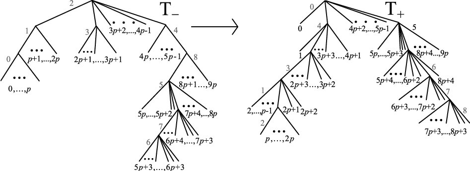
The minimal tree-pair diagram representative of an element of this form can be seen in Figure 7. This family of seesaw words will be denoted ${\mathcal{S}}$ .

Figure 7. Minimal tree-pair diagram representative of an arbitrary seesaw element in the family

{\mathcal{S}}

. The letter

m

denotes the number of carets of type

{\mathcal{L}_{\rm L}}

S_{-}

and the letter

n

denotes the number of carets of type

{\mathcal{R}}

on the right side of

S_{-}

which are not of type

{\mathcal{R}_{\emptyset}}

The proofs that follow will be concerned entirely with showing that all elements with minimal tree-pair diagram representative of the form given in Figure 7 are seesaw words with respect to $x_{0}$ . The algebraic expression is entirely determined by the minimal tree-pair diagram; to see how this algebraic expression can be obtained from the tree-pair diagram given in Figure 7, see the section on normal forms of $F(p+1)$ in [16]. This family ${\mathcal{S}}$ is a generalization of the family of seesaw words introduced by Cleary and Taback in [10].

For our proof, we take arbitrary $w=(S_{-},S_{+})\in{\mathcal{S}}$ . First we prove that $w$ satisfies part 1 of the definition of seesaw words with respect to $x_{0}\in X$ .

Lemma 2.1.

|wx_{0}^{\pm q}|=|w|-q\hbox{ for all }q\hbox{ such that }0<q<m-1,n-1

where $m$ denotes the number of carets of type ${\mathcal{L}_{\rm L}}$ in $S_{-}$ and $n$ denotes the number of carets of type ${\mathcal{R}}$ on the right side of $S_{-}$ which are not type ${\mathcal{R}_{\emptyset}}$ .

Proof.

We prove this by induction. Throughout this proof, we let $(S^{q}_{-},S^{q}_{+})$ denote $((Sx^{-q})_{-},(Sx^{-q})_{+})$ and we let $(R^{q}_{-},R^{q}_{+})$ denote $((Sx^{q})_{-},(Sx^{q})_{+})$ , where $q>0$ in both cases. Our inductive hypothesis assumes that $wx_{0}^{q}$ and $wx_{0}^{-q}$ have minimal tree-pair diagram representatives of the form given in Figures 8 and 9 respectively.

(1)

$|wx_{0}^{-q}|$ : We begin by considering the case when $q=1$ . Performing the multiplication $wx_{0}^{-1}$ using the minimal tree-pair diagram representatives of $w$ and $x_{0}^{-1}$ in Figures 7 and 3 respectively, we obtain Figure 8 (when $q=1$ ); $(S^{1}_{-},S^{1}_{+})$ is minimal because there are only two exposed carets in $S^{1}_{+}$ : the carets with leftmost leaf index numbers $p$ and $np^{2}+(m+n)p$ , but neither of the leaves with these index numbers in $S^{1}_{-}$ is the leftmost leaf of an exposed caret.

Our inductive hypothesis will be that $|wx_{0}^{-q}|=|w|-q$ for some $q$ such that $0<q<m-1,n-1$ and that $wx_{0}^{-q}$ has minimal tree-pair diagram representative $(S^{q}_{-},S^{q}_{+})$ (see Figure 8). Now we assume our hypotheses hold for some $q=j-1$ such that $0<j<n-2$ and we consider what happens when we multiply $wx_{0}^{-(j-1)}$ by $x_{0}^{-1}$ on the right. By our inductive hypothesis, the tree-pair diagram in Figure 8 is the minimal representative of $wx_{0}^{-(j-1)}$ when $q=j-1$ . Because $wx_{0}^{-(j-1)}$ and $x_{0}^{-1}$ satisfy the subtree condition, the positive tree $S^{j-1}_{+}$ remains unchanged after multiplication by $x_{0}^{-1}$ (see Remark 1.3). So we consider which changes $x_{0}^{-1}$ makes to the negative tree.

By looking at Figures 6 and 8 which represent $wx_{0}^{-(j-1)}$ and $x_{0}^{-1}$ respectively, we can see that multiplying $wx_{0}^{-(j-1)}$ by $x_{0}^{-1}$ changes $\wedge_{m+2+(j-1)(p+1)}$ (the rightmost child of the root) in $S_{-}^{j-1}$ from type ${\mathcal{R}}_{1}$ to type ${\mathcal{L}_{\rm L}}$ . This is the only change in the negative tree. So we can see that the resulting tree-pair diagram representative for $wx_{0}^{-j}$ will have $\wedge_{m+2+(j-1)(p+1)}$ as the root caret and $\wedge_{m+2+(j-2)(p+1)}$ as the leftmost child of the root. The relative location of all other carets in the tree will be identical to their placement in the minimal tree-pair diagram representative for $wx_{0}^{-(j-1)}$ . So it is clear that Figure 8 (when $q=j$ ) is a tree-pair diagram representative for $wx_{0}^{-j}$ . Now we need only show that it is minimal; we note that any carets which are exposed in $(S^{j}_{-},S^{j}_{+})$ would also have been exposed in $(S^{j-1}_{-},S^{j-1}_{+})$ , so minimality of $(S_{-}^{j-1},S_{+}^{j-1})$ implies minimality of $(S_{-}^{j},S_{+}^{j})$ .

Now we consider the effect of multiplication of $wx_{0}^{-(j-1)}$ by $x_{0}^{-1}$ on the length of $wx_{0}^{-(j-1)}$ . The caret $\wedge_{m+2+(j-1)(p+1)}$ will always be a successor of the caret $\wedge_{m}$ in both $S_{+}^{j-1}$ and $S_{+}^{j}$ , and the only successors of $\wedge_{m}$ in $S_{+}^{j-1}$ and $S_{+}^{j}$ which are not of type ${\mathcal{R}_{\rm R}}$ are $\wedge_{m+np+n}$ and $\wedge_{m+np+n+1}$ . Since $j<n$ , it is clear that $m+2+(j-1)(p+1)<m+np+n$ and therefore $\wedge_{m+2+(j-1)(p+1)}$ is of type ${\mathcal{R}_{\rm R}}$ in $S^{j-1}_{+}$ and $S_{+}^{j}$ . Therefore, this change in the caret $\wedge_{m+2+(j-1)(p+1)}$ in the negative tree from type ${\mathcal{R}}_{1}$ to type ${\mathcal{L}_{\rm L}}$ changes the pairing from ( ${\mathcal{R}}_{1}$ , ${\mathcal{R}_{\rm R}}$ ), which has weight 2, to ( ${\mathcal{L}_{\rm L}}$ , ${\mathcal{R}_{\rm R}}$ ), which has weight 1 (see Table 1). So $|wx_{0}^{-j}|=|wx_{0}^{-(j-1)}|-1$ . And since by our inductive hypotheses $|wx_{0}^{-(j-1)}|=|w|-(j-1)$ ,

$|wx_{0}^{-j}|=|w|-(j-1)-1=|w|-j\hbox{ for all }j\hbox{ s.t. }0<j<n-1$
(2)

$|wx_{0}^{q}|$ : The proof that $|wx_{0}^{q}|=|w|-q$ is similar to the proof that $|wx_{0}^{-q}|=|w|-q$ . The primary difference is that the caret in $(R_{-}^{j-1},R_{+}^{j-1})$ in Figure 9 whose type is changed by multiplication by $x_{0}$ is $\wedge_{m-(j-1)}$ (the root caret) in $R_{-}^{j-1}$ , which is changed from type ${\mathcal{L}_{\rm L}}$ to type ${\mathcal{R}_{\rm R}}$ (or ${\mathcal{R}_{\it p}}$ in the case $j=1$ ). In the same way as for the $x_{0}^{-1}$ case, this leads to the conclusion that Figure 9 is a minimal tree-pair diagram representative of $wx_{0}^{j}$ when $q=j$ . Then to compute the effect of multiplication by $x_{0}$ on length, we note that the caret $\wedge_{m-(j-1)}$ in $R_{+}^{j-1}$ or $R_{+}^{j}$ will always be of type ${\mathcal{L}_{\rm L}}$ for any given $j=1,\dots,m-2$ because $\wedge_{m-(j-1)}$ is a predecessor of the root $\wedge_{m}$ in $R_{+}^{j-1}$ and $R_{+}^{j}$ since $m-(j-1)<m$ and, and the only predecessors of the root in $R_{+}^{j-1}$ or $R_{+}^{j}$ which are not of type ${\mathcal{L}_{\rm L}}$ are $\wedge_{1}$ and $\wedge_{0}$ . Since $j\leq m-2$ guarantees that $m-(j-1)>1$ for all possible $j$ , $\wedge_{m-(j-1)}\neq\wedge_{1}$ or $\wedge_{0}$ . Therefore, this change in the caret $\wedge_{m-(j-1)}$ from type ${\mathcal{L}_{\rm L}}$ to type ${\mathcal{R}_{\rm R}}$ (or ${\mathcal{R}_{\it p}}$ when $j=1$ ) changes the pairing from ( ${\mathcal{L}_{\rm L}}$ , ${\mathcal{L}_{\rm L}}$ ), which has weight 2, to ( ${\mathcal{R}_{\rm R}}$ , ${\mathcal{L}_{\rm L}}$ ) (or ( ${\mathcal{R}_{\it p}}$ , ${\mathcal{L}_{\rm L}}$ ) when $j=1$ ), which has weight 1 (see Table 1). Then similarly to the $x_{0}^{-1}$ case, we can use induction to conclude that $|wx_{0}^{q}|=|w|-q$ and that Figure 9 is a minimal tree-pair diagram representative of $wx_{0}^{q}$ for all $q$ such that $0\leq q<m-1$ .

∎

Now we show that all $w\in\mathcal{S}$ satisfy part 2 of the definition of a seesaw word by considering the “action” of each $g\in X\cup X^{-1}$ on $wx_{0}^{\pm q}$ for arbitrary $q$ such that $0\leq q<m-1,n-1$ , and showing that this “action” always results in increased length.

Lemma 2.2.

For $w\in{\mathcal{S}}$ , $\epsilon\in\{-1,1\}$ , and arbitrary $q$ s.t. $0<|q|<m-1,n-1$ ,

|wx_{0}^{\epsilon q}g|\geq|wx_{0}^{\epsilon q}|

for all $g\in X\cup X^{-1}$ .

Proof.

We consider each possible combination of values of $\epsilon$ and $g$ :

(1)

$|wx_{0}^{-q}x_{i}^{\pm 1}|$ , $i\in\{1,2,...,p\}$ : First we note that $wx_{0}^{-q}$ and $x_{i}^{\pm 1}$ when $0\leq q<m-1,n-1$ and $i=1,2,...,p$ satisfy both the subtree and minimality conditions of Theorem 1.2 except when $q=0$ and $i=1,...,p-1$ . So only one caret will change type in the negative tree and the positive tree will remain unchanged after multiplication in these cases.
We begin with the case $q=0$ .
1. (a)
  
  $|wx_{i}^{-1}|$ : Multiplying $w$ by $x_{i}^{-1}$ changes $\wedge_{m+2}$ from type ${\mathcal{R}}_{1}$ to type ${\mathcal{M}}^{\it i}_{1}$ and changes no other caret types. Since all the carets in $S_{+}$ and $S_{+}^{1}$ which succeed $\wedge_{m}$ and precede $\wedge_{m+np+n}$ have type ${\mathcal{R}_{\rm R}}$ and $m<m+2<m+np+n$ , $\wedge_{m+2}$ is of type ${\mathcal{R}_{\rm R}}$ in $S_{+}$ and $S_{+}^{1}$ . So the change in the type pair of $\wedge_{m+2}$ goes from ( ${\mathcal{R}}_{1}$ , ${\mathcal{R}_{\rm R}}$ ) which has weight 2 to type ( ${\mathcal{M}}^{\it i}_{1}$ , ${\mathcal{R}_{\rm R}}$ ) which has weight 3, and clearly $|wx_{i}^{-1}|>|w|$ .
2. (b)
  
  $|wx_{i}|$ : Multiplying $w$ by $x_{i}$ when $i=1,...,p-1$ does not satisfy the subtree condition and therefore by Theorem 1.3, $|wx_{i}|>|w|$ . Multiplying $w$ by $x_{p}$ changes $\wedge_{m+1}$ from type ${\mathcal{M}^{\it p}_{\emptyset}}$ to type ${\mathcal{R}_{\rm R}}$ and changes no other caret types. Since $m<m+1<m+np+n$ , $\wedge_{m+1}$ is of type ${\mathcal{R}_{\rm R}}$ in $S_{+}$ and $R_{+}^{1}$ . So this change in the type pair of $\wedge_{m+1}$ goes from ( ${\mathcal{M}^{\it p}_{\emptyset}}$ , ${\mathcal{R}_{\rm R}}$ ) which has weight 1 to ( ${\mathcal{R}_{\rm R}}$ , ${\mathcal{R}_{\rm R}}$ ) which has weight 2, so $|wx_{p}|>|w|$ .
Now we consider multiplying $wx_{0}^{-q}$ for $0<q<m-1,n-1$ by $x_{i}^{\pm 1}$ for $i=1,2,...,p$ , when both conditions of Theorem 1.2 are met.
1. (a)
  
  $|wx_{0}^{-q}x_{i}^{-1}|$ : Multiplying $wx_{0}^{-q}$ by $x_{i}^{-1}$ changes $\wedge_{m+2+q(p-1)}$ (the right child of the root) in $S_{-}^{q}$ from type ${\mathcal{R}}_{1}$ to type ${\mathcal{M}}^{\it i}_{1}$ . In $S_{+}^{q}$ and $S_{+}^{q+1}$ , all carets which succeed $\wedge_{m}$ and precede $\wedge_{m+np+n}$ have type ${\mathcal{R}_{\rm R}}$ , so since $m<m+2+q(p-1)<m+np+n$ (because $q<n-1$ ), $\wedge_{m+2+q(p-1)}$ is of type ${\mathcal{R}_{\rm R}}$ in $S_{+}^{q}$ and $S_{+}^{q+1}$ . So this multiplication changes the type pair of $\wedge_{m+2+q(p-1)}$ from ( ${\mathcal{R}}_{1}$ , ${\mathcal{R}_{\rm R}}$ ), which has weight 2, to ( ${\mathcal{M}}^{\it i}_{1}$ , ${\mathcal{R}_{\rm R}}$ ), which has weight 3. So $|wx_{0}^{-q}\mbox{$x_{i}$}^{-1}|=|w|-q+1$ .
2. (b)
  
  $|wx_{0}^{-q}x_{i}|$ : Multiplying $wx_{0}^{-q}$ by $x_{i}$ changes $\wedge_{m+2+(q-1)(p-1)+i}$ (the $ith$ child of the root) in $S_{-}^{q}$ from type ${\mathcal{M}^{\it i}_{\emptyset}}$ to type ${\mathcal{R}}_{i+1}$ when $i<p$ and to type ${\mathcal{R}_{\rm R}}$ when $i=p$ . Again, since $m<m+2+(q-1)(p-1)+i<m+np+n$ (because $q<n-1$ ), $\wedge_{m+2+(q-1)(p-1)+i}$ is of type ${\mathcal{R}_{\rm R}}$ in $R_{+}^{q}$ and $R_{+}^{q+1}$ . So this multiplication changes the type pair of $\wedge_{m+2+(q-1)(p-1)+i}$ from ( ${\mathcal{M}^{\it i}_{\emptyset}}$ , ${\mathcal{R}_{\rm R}}$ ), which has weight 1, to ( ${\mathcal{R}}_{i+1}$ , ${\mathcal{R}_{\rm R}}$ ) when $i<p$ and ( ${\mathcal{R}_{\rm R}}$ , ${\mathcal{R}_{\rm R}}$ ) when $i=p$ , both of which have weight 2. So $|wx_{0}^{-q}\mbox{$x_{i}$}|=|w|-q+1$ .
(2)
$|wx_{0}^{q}x_{i}^{\pm 1}|$ , $i\in\{1,2,...,p\}$ : Now we consider multiplying $wx_{0}^{q}$ for $0<q<m-1,n-1$ by $x_{i}^{\pm 1}$ for $i=1,2,...,p$ . First we note that $wx_{0}^{q}$ and $x_{i}^{-1}$ when $0\leq q<m-1,n-1$ and $i=1,2,...,p$ satisfy both the subtree and minimality conditions of Theorem 1.2. So only one caret will change type in the negative tree and the positive tree will remain unchanged after multiplication in this case.
1. (a)
  
  $|wx_{0}^{q}x_{i}^{-1}|$ : If we let $i=1,\dots,p$ , multiplying $wx_{0}^{q}$ by $x_{i}^{-1}$ changes the rightmost child of the root, which is $\wedge_{m-q+1}$ when $q>0$ and $\wedge_{m+2}$ when $q=0$ . When $q=0$ , we can conclude that $\wedge_{m+2}$ is of type ${\mathcal{R}_{\rm R}}$ in both $S_{+}$ and $R_{+}^{1}$ (since $m<m+2<m+np+n$ ), and $\wedge_{m+2}$ is changed from type ${\mathcal{R}}_{1}$ to type ${\mathcal{M}}^{\it i}_{1}$ , changing the type pairing from ( ${\mathcal{R}}_{1}$ , ${\mathcal{R}_{\rm R}}$ ) which has weight 2 to ( ${\mathcal{M}}^{\it i}_{1}$ , ${\mathcal{R}_{\rm R}}$ ) which has weight 3. When $q>0$ , we can conclude that $\wedge_{m-q+1}$ is of type ${\mathcal{L}_{\rm L}}$ in both $R_{+}^{q}$ and $R_{+}^{q+1}$ since all carets which succeed $\wedge_{1}$ and precede $\wedge_{m+1}$ in $R_{+}^{q}$ and $R_{+}^{q+1}$ are of type ${\mathcal{L}_{\rm L}}$ and clearly $1<m-q+1<m+1$ (since $q<m-1$ ). When $q=1$ , $\wedge_{m-q+1}$ is changed from type ${\mathcal{R}_{\rm R}}$ to type ${\mathcal{M}^{\it i}_{\emptyset}}$ , changing the type pairing from ( ${\mathcal{R}_{\it p}}$ , ${\mathcal{L}_{\rm L}}$ ) or ( ${\mathcal{R}_{\rm R}}$ , ${\mathcal{L}_{\rm L}}$ ), both of which have weight 1, to ( ${\mathcal{M}^{\it i}_{\emptyset}}$ , ${\mathcal{L}_{\rm L}}$ ) which has weight 2. So $|wx_{0}^{q}\mbox{$x_{i}$}^{-1}|=|w|-q+1$ .
2. (b)
  $|wx_{0}^{q}x_{i}|$ , $i\in\{1,2,...,p\}$ :
  1. (i)
    
    $|wx_{0}^{q}x_{i}|$ , $i\in\{1,2,...,p\}$ , except when $q=0$ and $i=p$ : In this case, multiplying $wx_{0}^{q}$ by $x_{i}$ does not satisfy the required conditions of Theorem 1.2 because we must add a caret before we can complete the multiplication, so we know from Theorem 1.3 that $|wx_{0}^{q}\mbox{$x_{i}$}|>|wx_{0}^{q}|$ in this case.
  2. (ii)
    
    $|wx_{0}^{q}x_{p}|$ : When $q=0$ , $wx_{0}^{q}$ and $x_{p}$ satisfy the required subtree and minimality conditions of Theorem 1.2 and therefore only one caret changes type in the negative tree and the positive tree remains unchanged. The caret $\wedge_{m+1}$ is changed from type ${\mathcal{M}^{\it p}_{\emptyset}}$ to type ${\mathcal{R}_{\rm R}}$ . Since $m<m+1<m+np+n$ , it is clear that $\wedge_{m+1}$ is of type ${\mathcal{R}_{\rm R}}$ in $S_{+}$ and $R_{+}^{1}$ , and so the change in type pairing goes from ( ${\mathcal{M}^{\it p}_{\emptyset}}$ , ${\mathcal{R}_{\rm R}}$ ) which has weight 1 to ( ${\mathcal{R}_{\rm R}}$ , ${\mathcal{R}_{\rm R}}$ ) which has weight 2. So we can conclude that that $|wx_{0}^{q}\mbox{$x_{i}$}|>|wx_{0}^{q}|$ in this case.

∎

Proof of Theorem 2.1.

This proof follows immediately from Lemma 2.1, Lemma 2.2, and Definition 1.2. So all $w\in{\mathcal{S}}$ are seesaw words, and we can create such words with any given swing $k$ (where $0<k<min\{m-1,n-1\}$ ) by choosing $m$ and $n$ such that $m,n>k+1$ . ∎

Corollary 2.1.

Thompson’s group $F(p+1)$ contains seesaw words of arbitrarily large swing with respect to $x_{0}\in X$ .

2.2. Consequences

Lemma 2.3.

Given any constant k, there exists a word $w\in{\mathcal{S}}$ such that no geodesics paths from the identity to $wx_{0}$ , $w$ , or $wx_{0}^{-1}$ satisfy the k-fellow traveler property.

Proof.

This holds for the same reasons that Prop. 4.2 in [10] holds for $p=1$ . ∎

Theorem 2.2.

Thompson’s group $F(p+1)$ is not combable by geodesics.

Proof.

This holds for the same reasons that Theorem 4.2 in [10] holds for $p=1$ . ∎

Theorem 2.3 (Theorem 30 in [6]).

A group $G$ generated by a finite set $X$ with seesaw elements of arbitrary swing w.r.t. $X$ has no regular language of geodesics.

Corollary 2.2.

There does not exist a regular language of geodesics for $F(p+1)$ with respect to $X$ .

3. Dead ends exist in Thompson’s group $F(p+1)$

Cleary and Taback in [9] have shown that $F(2)$ has dead ends, and that all these dead ends have depth 2. In this section we use a similar approach to extend their results to $F(p+1)$ for all $p\in\mathbb{N}$ .

3.1. Dead ends in $F(p+1)$

The proofs in this section will contain many tree-pair diagrams which use the following notational convention.

Notation 3.1 (Subtrees in tree-pair diagrams).

When depicting tree-pair diagrams, the symbol indicates the presence of a non-empty subtree, and the the symbol indicates the presence of a (possibly empty) subtree. When neither of these symbols are used, it is assumed that there is no subtree present.

Now we proceed to show that elements of $F(p+1)$ are dead ends if and only if they have a minimal tree-pair diagram representative with a specific form.

Theorem 3.1.

All dead ends in $F(p+1)$ under $X$ have minimal tree-pair diagrams of the form given in Figure 10.

We note that in Theorem 3.1 we mean that the minimal form of the dead end tree-pair diagram representative must include all of the carets explicitly given in Figure 10, so, for example, at least one of the subtrees labeled $f_{1},...,f_{p}$ in $T_{-}$ and at least one of the subtrees labeled $f_{1}^{\prime},...,f_{p}^{\prime}$ in $T_{+}$ are non-empty because otherwise $\wedge_{F}$ would cancel. The proof of this theorem is based upon recognizing how the “action” of each $g\in X\cup X^{-1}$ affects an arbitrary tree-pair diagram $(T_{-},T_{+})$ .

Remark 3.1.

The negative tree of any $(p+1)$ –ary tree-pair diagram can be written in the (possibly non-minimal) form given by Figure 11, and for any negative tree in this form, the “action” of any $g\in X\cup X^{-1}$ on $T_{-}$ will change only one caret type in that tree (This is because the only other changes in type that can occur when multiplying by a generator are caused by the addition of carets to the tree-pair diagram, but by definition, negative trees in this form will belong to tree-pair diagrams to which all carets needed in order to multiply by a generator or its inverse have already been added - see Theorem 1.2 and Remark 1.3).

The “action” of $g$ on this negative tree will produce the following caret type change (see Figure 6):

(1)

$x_{0}$ takes the type of $\wedge_{B}$ from ${\mathcal{L}_{\rm L}}$ to ${\mathcal{R}}$ .
(2)

$x_{0}^{-1}$ takes the type of $\wedge_{E}$ from ${\mathcal{R}}$ to ${\mathcal{L}_{\rm L}}$ .
(3)

$x_{i}$ for $i=1,...,p-1$ takes the type of $\wedge_{C^{i}}$ from ${\mathcal{M}^{\it i}}$ to ${\mathcal{R}}$ .
(4)

$x_{i}^{-1}$ for $i=1,...,p-1$ takes the type of $\wedge_{E}$ from ${\mathcal{R}}$ to ${\mathcal{M}^{\it i}}$ .
(5)

$x_{p}$ takes the type of $\wedge_{D}$ from ${\mathcal{M}^{\it p}}$ to ${\mathcal{R}}$ .
(6)

$x_{p}^{-1}$ takes the type of $\wedge_{E}$ from ${\mathcal{R}}$ to ${\mathcal{M}^{\it p}}$ .

Because a dead end $w$ by definition must not increase in length when multiplied by $g\in X\cup X^{-1}$ (by Theorem 1.3), the product $wg$ must satisfy the subtree condition for any $g$ .

Lemma 3.1.

All dead ends must have a minimal tree-pair diagram with negative tree of the form given by Figure 11, and any dead end $w$ must satisfy the subtree and minimality conditions with respect to all possible $g\in X\cup X^{-1}$ .

Proof.

A minimal $(p+1)$ –ary tree-pair diagram representing an arbitrary element $x\in F(p+1)$ will have a negative tree of this form if and only if $x$ and $g\in X\cup X^{-1}$ satisfy the subtree condition (see Remark 3.1). For an arbitrary dead end $w$ , we cannot have $|wg|>|w|$ , so by Theorem 1.3, $w$ must satisfy the subtree conditions with respect to all possible $g$ .

The fact that $w=(T_{-},T_{+})$ satisfies the minimality condition with respect to all possible $g$ follows directly from the fact that it satisfies the subtree condition. The subtree condition implies that $T_{+}=(Tg)_{+}$ , and therefore, the only way in which exposed caret pairs may exist in $((Tg)_{-},(Tg)_{+})$ , is if the “action” of $g$ on $(T_{-},T_{+})$ causes carets to be exposed in $(Tg)_{-}$ which were not exposed in $T_{-}$ . However, if we consider the “action” of each $g$ on the negative tree of $w$ , which must be of the form given in Figure 11, we can see that for all $g\in X\cup X^{-1}$ , the only carets which will be exposed in $(Tg)_{-}$ are those which are also exposed in $T_{-}$ (see Figure 6, or consider Figures 12, 15, 13, 16, 14 and 17 which follow). Therefore $((Tg)_{-},(Tg)_{+})$ is minimal for all $g$ . ∎

Corollary 3.1.

For all dead ends $w=(T_{-},T_{+})$ and all $g\in X\cup X^{-1}$ , the “action” of $g$ on $(T_{-},T_{+})$ only changes the type of one caret in $T_{-}$ and leaves the types of all carets in $T_{+}$ unchanged.

Proof.

This follows immediately from Lemma 3.1, Remark 1.3 and Theorem 1.2. ∎

So now we can proceed to prove Theorem 3.1 by observing which caret changes type in the tree-pair diagram when each $g$ “acts” on an arbitrary dead end $w=(T_{-},T_{+})$ and then enumerating those conditions which must be met by $(T_{-},T_{+})$ in order for this type change to result in a decrease in length (we note that length cannot remain unchanged after multiplication by $g$ because in $F(p+1)$ all relators are of even length). By showing that these conditions will be met if and only if $w$ satisfies those conditions laid out in Theorem 3.1, we will conclude our proof of the theorem. Before continuing with our proof, we first introduce some notation.

Notation 3.2 ( $\tau(\wedge_{j})$ and $\Delta_{g}(\wedge_{j})$ ).

$\tau_{T_{+}}(\wedge_{j})$ and $\tau_{(T_{-},T_{+})}(\wedge_{j})$ represent the type of the caret $\wedge_{j}$ in the tree $T_{+}$ and the the type pair of the caret pair $\wedge_{j}$ in the tree-pair diagram $(T_{-},T_{+})$ , respectively.

$\Delta_{g}(\wedge_{j})$ denotes the change in weight of the caret pair $\wedge_{j}$ during multiplication by some $g\in X\cup X^{-1}$ , where the original tree-pair diagram and the resulting tree-pair diagram should be clear from the context.

Proof of Theorem 3.1.

We consider multiplying our dead end element $w=(T_{-},T_{+})$ by each $g\in X\cup X^{-1}$ and enumerate which caret in the negative tree has its type changed by this multiplication and the effect of this change on the length of the element (see Table 1).

For a clearer organizational structure, we organize this process by the caret in $T_{-}$ which is affected by the multiplication. The labeled carets in $T_{-}$ are (see Figure 11): $\wedge_{A},\wedge_{B}\wedge_{C^{i}}\hbox{ for }i=1,...,p-1,\wedge_{D},\wedge_{E},\wedge_{F}$ . To see which $g$ affects which caret pair in $(T_{-},T_{+})$ , we consult Remark 3.1.

(1)

Conditions on $\wedge_{A}$ in $(T_{-},T_{+})$ : We know from Remark 3.1 that there is no $g\in X\cup X^{-1}$ which will change the type of $\wedge_{A}$ in the negative tree, so we have no conditions on the type of this caret unless they are imposed by the required types of other carets within the tree. By definition $\wedge_{A}$ is of type ${\mathcal{L}}$ in $T_{-}$ . In $T_{+}$ , the only conditions on $\wedge_{A}$ will come from the conditions imposed on $\wedge_{B}$ (see (2)); because $\wedge_{B}$ in $T_{+}$ must be of type ${\mathcal{L}}$ and since $\wedge_{A}$ is a predecessor of $\wedge_{B}$ , $\wedge_{A}$ in $T_{+}$ must be of type ${\mathcal{L}}$ or of type ${\mathcal{M}}$ with an ancestor of type ${\mathcal{L}}$ .

(2)

Conditions on $\wedge_{B}$ in $(T_{-},T_{+})$ : We know from Remark 3.1 that only $x_{0}$ will change the type of $\wedge_{B}$ in the negative tree, from type ${\mathcal{L}_{\rm L}}$ to type ${\mathcal{R}}$ . If we look at $(T_{-},T_{+})$ , we can see that in this case we can compute the types more specifically: $x_{0}$ will change the type of $\wedge_{B}$ in the negative tree from type ${\mathcal{L}_{\rm L}}$ to type ${\mathcal{R}}_{1}$ because $\wedge_{B}$ ’s leftmost child successor is $\wedge_{C^{1}}$ , which is of type $\mbox{${\mathcal{M}}$}^{1}$ (see Figure 12). Table 2 lists the change in weight (taken from Table 1) of this caret pair for each possible caret type pair of $\wedge_{B}$ . From this table we conclude that $\wedge_{B}$ in $T_{+}$ must be of type ${\mathcal{L}_{\rm L}}$ because this is the only caret pairing in $(T_{-},T_{+})$ for $\wedge_{B}$ which will result in $|wx_{0}|<|w|$ .

Table 2. How

x_{0}

“acts” on

w(\wedge_{B})

in arbitrary dead end

w=(T_{-},T_{+})

, listed by possible types of

\wedge_{B}\in T_{+}

. Here

\tau_{T_{-}}(\wedge_{B})=\mbox{${\mathcal{L}_{\rm L}}$}

$\tau_{T_{+}}(\wedge_{B})$	$\tau_{(T_{-},T_{+})}(\wedge_{B})$	$\tau_{((Tx_{0})_{-},(Tx_{0})_{+})}(\wedge_{B})$	$\Delta_{x_{0}}(\wedge_{B})$
${\mathcal{L}_{\rm L}}$	( ${\mathcal{L}_{\rm L}}$ , ${\mathcal{L}_{\rm L}}$ )	( ${\mathcal{R}}_{1}$ , ${\mathcal{L}_{\rm L}}$ )	-1
${\mathcal{R}_{\emptyset}}$	( ${\mathcal{L}_{\rm L}}$ , ${\mathcal{R}_{\emptyset}}$ )	( ${\mathcal{R}}_{1}$ , ${\mathcal{R}_{\emptyset}}$ )	1
${\mathcal{R}_{\rm R}}$	( ${\mathcal{L}_{\rm L}}$ , ${\mathcal{R}_{\rm R}}$ )	( ${\mathcal{R}}_{1}$ , ${\mathcal{R}_{\rm R}}$ )	1
${\mathcal{R}_{\it j}}$	( ${\mathcal{L}_{\rm L}}$ , ${\mathcal{R}_{\it j}}$ )	( ${\mathcal{R}}_{1}$ , ${\mathcal{R}_{\it j}}$ )	1
${\mathcal{M}^{\it i}_{\emptyset}}$	( ${\mathcal{L}_{\rm L}}$ , ${\mathcal{M}^{\it i}_{\emptyset}}$ )	( ${\mathcal{R}}_{1}$ , ${\mathcal{M}^{\it i}_{\emptyset}}$ )	1
${\mathcal{M}^{\it i}_{\it j}}$	( ${\mathcal{L}_{\rm L}}$ , ${\mathcal{M}^{\it i}_{\it j}}$ )	( ${\mathcal{R}}_{1}$ , ${\mathcal{M}^{\it i}_{\it j}}$ )	1

(3)

Conditions on $\wedge_{C^{i}}$ in $(T_{-},T_{+})$ for $i=1,2,...,p-1$ : We know from Remark 3.1 that only $x_{i}$ will change the type of $\wedge_{C^{i}}$ in the negative tree, from type ${\mathcal{M}^{\it i}}$ to type ${\mathcal{R}}$ (see Figure 13). First we enumerate the conditions imposed by the specific subtype of $\wedge_{C^{i}}$ in $T_{-}$ on the specific subtype of $\wedge_{C^{i}}$ in $(Tx_{i})_{-}$ (in Figure 13). First we note that in both $T_{-}$ and $(Tx_{i})_{-}$ , in $\wedge_{C^{i}}$ , the child carets in the subtrees $c_{1}^{i},...,c_{p-i+1}^{i}$ (if they are nonempty) will be predecessors of $\wedge_{C^{i}}$ and the child carets in the subtrees $c_{p-i+2}^{i},...,c_{p+1}^{i}$ (if they are nonempty) will be successors of $\wedge_{C^{i}}$ (see Figure 5). Additionally, the root caret of the subtrees $c_{1}^{i},...,c_{p-i+1}^{i}$ (if they exist) will have caret types $\mbox{${\mathcal{M}}$}^{i},...,\mbox{${\mathcal{M}}$}^{p}$ respectively, and the root carets of the subtrees $c_{p-i+2}^{i},...,c_{p+1}^{i}$ (if they exist) will have caret types $\mbox{${\mathcal{M}}$}^{1},...,\mbox{${\mathcal{M}}$}^{i}$ respectively (see Figure 4).

(a)

If $\tau_{T_{-}}(\wedge_{C^{i}})=\mbox{${\mathcal{M}^{\it i}_{\emptyset}}$}$ , then the subtrees $c_{p-i+2}^{i},...,c_{p+1}^{i}$ are all empty, which implies that $\wedge_{C^{i+1}}$ is the leftmost child successor of $\wedge_{C^{i}}$ . Since $\tau(\wedge_{C^{i+1}})=\mbox{${\mathcal{M}}$}^{i+1}$ , $\tau_{(Tx_{i})_{-}}(\wedge_{C^{i}})=\mbox{${\mathcal{R}}_{i+1}$}$ .
(b)

If $\tau_{T_{-}}(\wedge_{C^{i}})=\mbox{${\mathcal{M}^{\it i}_{\it j}}$}$ , then the leftmost child successor of $\wedge_{C^{i}}$ in $T_{-}$ is the root caret of the subtree $c_{j}^{i}$ , which implies that the subtrees $c_{p-i+2}^{i},...,c_{j-1}^{i}$ are all empty. So the leftmost child successor of $\wedge_{C^{i}}$ in $(Tx_{i})_{-}$ will also be the root of subtree $c_{j}^{i}$ , which is of type $\mbox{${\mathcal{M}}$}^{j}$ , so $\tau_{(Tx_{i})_{-}}(\wedge_{C^{i}})=\mbox{${\mathcal{R}_{\it j}}$}$ .

Table 3 lists the change in weight (taken from Table 1) of this caret pair $\wedge_{C^{i}}$ when $\tau_{T_{-}}(\wedge_{C^{i}})=\mbox{${\mathcal{M}^{\it i}_{\emptyset}}$}$ ; When $\tau_{T_{-}}(\wedge_{C^{i}})=\mbox{${\mathcal{M}^{\it i}_{\it j}}$}$ , the change in caret type of $\wedge_{C^{i}}$ from ${\mathcal{M}^{\it i}_{\it j}}$ to ${\mathcal{R}_{\it j}}$ results in a decrease in caret weight no matter what the type of $\wedge_{C^{i}}$ in $T_{+}$ , so we conclude that if $\tau_{T_{-}}(\wedge_{C^{i}})=\mbox{${\mathcal{M}^{\it i}_{\it j}}$}$ , then $\wedge_{C^{i}}$ in $T_{+}$ may be of any type. If $\tau_{T_{-}}(\wedge_{C^{i}})=\mbox{${\mathcal{M}^{\it i}_{\emptyset}}$}$ , then we can see from Table 3 that $\wedge_{C^{i}}$ in $T_{+}$ may be of type ${\mathcal{L}_{\rm L}}$ , ${\mathcal{R}_{\it k}}$ or ${\mathcal{M}^{\it k}_{\emptyset}}$ , or ${\mathcal{M}^{\it r}_{\it s}}$ for $k,r,s\leq i$ .

Table 3. How

x_{i}

(for

i=1,2,...,p-1

), when

\tau_{T_{-}}(\wedge_{C^{i}})=\mbox{${\mathcal{M}^{\it i}_{\emptyset}}$}

, “acts” on

w(\wedge_{C^{i}})

in arbitrary dead end

w=(T_{-},T_{+})

, listed by possible types of

\wedge_{C^{i}}\in T_{+}

$\tau_{T_{+}}(\wedge_{C^{i}})$	$\tau_{(T_{-},T_{+})}(\wedge_{C^{i}})$	$\tau_{((Tx_{i})_{-},(Tx_{i})_{+})}(\wedge_{C^{i}})$	$\Delta_{x_{i}}(\wedge_{C^{i}})$
${\mathcal{L}_{\rm L}}$	( ${\mathcal{M}^{\it i}_{\emptyset}}$ , ${\mathcal{L}_{\rm L}}$ )	( ${\mathcal{R}}_{i+1}$ , ${\mathcal{L}_{\rm L}}$ )	-1
${\mathcal{R}_{\emptyset}}$	( ${\mathcal{M}^{\it i}_{\emptyset}}$ , ${\mathcal{R}_{\emptyset}}$ )	( ${\mathcal{R}}_{i+1}$ , ${\mathcal{R}_{\emptyset}}$ )	1
${\mathcal{R}_{\rm R}}$	( ${\mathcal{M}^{\it i}_{\emptyset}}$ , ${\mathcal{R}_{\rm R}}$ )	( ${\mathcal{R}}_{i+1}$ , ${\mathcal{R}_{\rm R}}$ )	1
${\mathcal{R}_{\it j}}$	( ${\mathcal{M}^{\it i}_{\emptyset}}$ , ${\mathcal{R}_{\it j}}$ )	( ${\mathcal{R}}_{i+1}$ , ${\mathcal{R}_{\it j}}$ )	${}^{-1\hbox{ for }j\leq i}_{\hbox{ }\hbox{ }1\hbox{ for }j>i}$
${\mathcal{M}^{\it k}_{\emptyset}}$	( ${\mathcal{M}^{\it i}_{\emptyset}}$ , ${\mathcal{M}^{\it k}_{\emptyset}}$ )	( ${\mathcal{R}}_{i+1}$ , ${\mathcal{M}^{\it k}_{\emptyset}}$ )	${}^{-1\hbox{ for }k\leq i}_{\hbox{ }\hbox{ }1\hbox{ for }k>i}$
$\mbox{${\mathcal{M}}$}^{l}_{m}$	( ${\mathcal{M}^{\it i}_{\emptyset}}$ , $\mbox{${\mathcal{M}}$}^{l}_{m}$ )	( ${\mathcal{R}}_{i+1}$ , $\mbox{${\mathcal{M}}$}^{l}_{m}$ )	${}^{-1\hbox{ for }l\leq i}_{\hbox{ }\hbox{ }1\hbox{ for }l>i}$

(4)

Conditions on $\wedge_{D}$ in $(T_{-},T_{+})$ : We know from Remark 3.1 that only $x_{p}$ will change the type of $\wedge_{D}$ in the negative tree, from type ${\mathcal{M}^{\it p}}$ to type ${\mathcal{R}}$ (see Figure 14). First we enumerate the conditions which determine the subtype of $\wedge_{D}$ in $T_{-}$ and the conditions imposed by that specific subtype of $\wedge_{D}$ in $T_{-}$ on the specific subtype of $\wedge_{D}$ in $(Tx_{i})_{-}$ in Figure 14. First we note that in both $T_{-}$ and $(Tx_{p})_{-}$ , in $\wedge_{D}$ , the child carets in the subtree $d_{0}$ (if nonempty) will be predecessors of $\wedge_{D}$ and the child carets in the subtrees $d_{1},...,d_{p}$ (if nonempty) will be successors of $\wedge_{D}$ (see Figure 5). Additionally, the root caret of the subtrees $d_{0},d_{1}...,d_{p}$ (if they exist) will have caret types $\mbox{${\mathcal{M}}$}^{p},\mbox{${\mathcal{M}}$}^{1},...,\mbox{${\mathcal{M}}$}^{p}$ respectively (see Figure 4).

(a)

If $d_{j}$ is a leaf for all $j\in\{1,...,p\}$ , then $\tau_{T_{-}}(\wedge_{D})=\mbox{${\mathcal{M}^{\it p}_{\emptyset}}$}$ , because $\wedge_{D}\in T_{-}$ will have no child successors (see Figure 3.1), and $\tau_{(Tx_{p})_{-}}(\wedge_{D})=\mbox{${\mathcal{R}_{\rm R}}$}$ or ${\mathcal{R}_{\emptyset}}$ since the leftmost child successor of $\wedge_{D}\in(Tx_{p})_{-}$ will be $\wedge_{E}$ , which will also be $\wedge_{D}$ ’s immediate successor (see Figure 14).
(b)

If there is a $j\in\{1,...,p\}$ such that $d_{j}$ is not a leaf, then $\tau_{T_{-}}(\wedge_{D})=\mbox{${\mathcal{M}^{\it p}_{\it i}}$}$ , where $i=min\{j|d_{j}\hbox{ is not a leaf}\}$ , and $\tau_{(Tx_{p})_{-}}(\wedge_{D})=\mbox{${\mathcal{R}_{\it i}}$}$ , because when $j<p$ , the root of the subtree $d_{i}$ will be the leftmost child successor of $\wedge_{D}$ in both $T_{-}$ and $(Tx_{p})_{-}$ , and will be of type $\mbox{${\mathcal{M}}$}^{i}$ in both trees, and when $j=p$ , the leftmost child successor of $\wedge_{D}$ will be the root of the subtree $d_{i}$ (type $\mbox{${\mathcal{M}}$}^{i}$ ) in $T_{-}$ and will be $\wedge_{E}$ (type ${\mathcal{R}}$ ) in $(Tx_{p})_{-}$ , and the immediate successor of $\wedge_{D}$ will be in the subtree $\mbox{${\mathcal{M}}$}^{i}$ in both trees (see Figures 4 and 5).

Table 4 lists the change in weight (taken from Table 1) of this caret pair $\wedge_{D}$ when $\tau_{T_{-}}(\wedge_{D})=\mbox{${\mathcal{M}^{\it p}_{\emptyset}}$}$ ; When $\tau_{T_{-}}(\wedge_{D})=\mbox{${\mathcal{M}^{\it p}_{\it j}}$}$ , the change in caret type of $\wedge_{D}$ from ${\mathcal{M}^{\it p}_{\it j}}$ to ${\mathcal{R}_{\it j}}$ decreases caret weight, no matter what the type of $\wedge_{D}$ in $T_{+}$ , so if $\tau_{T_{-}}(\wedge_{D})=\mbox{${\mathcal{M}^{\it p}_{\it j}}$}$ , then $\wedge_{D}$ in $T_{+}$ may be of any type. If $\tau_{T_{-}}(\wedge_{D})=\mbox{${\mathcal{M}^{\it p}_{\emptyset}}$}$ , then we can see from Table 4 that $\wedge_{D}$ in $T_{+}$ must be of type ${\mathcal{L}_{\rm L}}$ , ${\mathcal{R}_{\it j}}$ , ${\mathcal{M}^{\it k}_{\emptyset}}$ or ${\mathcal{M}^{\it k}_{\it l}}$ , where $j,k,l\in\{1,2,...,p\}$ . $|wx_{p}|<|w|$ .

Table 4. How

x_{p}

, when

\tau_{T_{-}}(\wedge_{D})=\mbox{${\mathcal{M}^{\it p}_{\emptyset}}$}

, “acts” on

w(\wedge_{D})

in arbitrary dead end

w=(T_{-},T_{+})

, listed by possible types of

\wedge_{D}\in T_{+}

. Case 1 is when

\tau_{(Tx_{p})_{-}}(\wedge_{D})=\mbox{${\mathcal{R}_{\rm R}}$}

, and case 2 is when

\tau_{(Tx_{p})_{-}}(\wedge_{D})=\mbox{${\mathcal{R}_{\emptyset}}$}

$\tau_{T_{+}}(\wedge_{D})$	$\tau_{(T_{-},T_{+})}(\wedge_{D})$	$\tau_{((Tx_{p})_{-},(Tx_{p})_{+})}(\wedge_{D})$		$\Delta_{x_{p}}(\wedge_{D})$
		case 1	case 2	case 1	case 2
${\mathcal{L}_{\rm L}}$	( ${\mathcal{M}^{\it p}_{\emptyset}}$ , ${\mathcal{L}_{\rm L}}$ )	( ${\mathcal{R}_{\rm R}}$ , ${\mathcal{L}_{\rm L}}$ )	( ${\mathcal{R}_{\emptyset}}$ , ${\mathcal{L}_{\rm L}}$ )	-1	-1
${\mathcal{R}_{\emptyset}}$	( ${\mathcal{M}^{\it p}_{\emptyset}}$ , ${\mathcal{R}_{\emptyset}}$ )	( ${\mathcal{R}_{\rm R}}$ , ${\mathcal{R}_{\emptyset}}$ )	( ${\mathcal{R}_{\emptyset}}$ , ${\mathcal{R}_{\emptyset}}$ )	1	1
${\mathcal{R}_{\rm R}}$	( ${\mathcal{M}^{\it p}_{\emptyset}}$ , ${\mathcal{R}_{\rm R}}$ )	( ${\mathcal{R}_{\rm R}}$ , ${\mathcal{R}_{\rm R}}$ )	( ${\mathcal{R}_{\emptyset}}$ , ${\mathcal{R}_{\rm R}}$ )	1	1
${\mathcal{R}_{\it j}}$	( ${\mathcal{M}^{\it p}_{\emptyset}}$ , ${\mathcal{R}_{\it j}}$ )	( ${\mathcal{R}_{\rm R}}$ , ${\mathcal{R}_{\it j}}$ )	( ${\mathcal{R}_{\emptyset}}$ , ${\mathcal{R}_{\it j}}$ )	-1	-1
${\mathcal{M}^{\it i}_{\emptyset}}$	( ${\mathcal{M}^{\it p}_{\emptyset}}$ , ${\mathcal{M}^{\it i}_{\emptyset}}$ )	( ${\mathcal{R}_{\rm R}}$ , ${\mathcal{M}^{\it i}_{\emptyset}}$ )	( ${\mathcal{R}_{\emptyset}}$ , ${\mathcal{M}^{\it i}_{\emptyset}}$ )	-1	-1
${\mathcal{M}^{\it i}_{\it j}}$	( ${\mathcal{M}^{\it p}_{\emptyset}}$ , ${\mathcal{M}^{\it i}_{\it j}}$ )	( ${\mathcal{R}_{\rm R}}$ , ${\mathcal{M}^{\it i}_{\it j}}$ )	( ${\mathcal{R}_{\emptyset}}$ , ${\mathcal{M}^{\it i}_{\it j}}$ )	-1	-1

(5)

Conditions on $\wedge_{E}$ in $(T_{-},T_{+})$ : We know from Remark 3.1 that $x_{i}^{-1}$ for $i=0,1,2,...,p$ will change the type of $\wedge_{E}$ in the negative tree, from type ${\mathcal{R}}$ to type ${\mathcal{L}_{\rm L}}$ when $i=0$ (see Figure 15) and ${\mathcal{M}^{\it i}}$ when $i>0$ (see Figures 16 and 17). First we enumerate the conditions that determine the subtype of $\wedge_{E}$ in $T_{-}$ (which is ${\mathcal{R}}$ ) and in $(Tx_{i})_{-}$ , (which is ${\mathcal{L}_{\rm L}}$ when $i=1$ and ${\mathcal{M}^{\it i}}$ when $i>0$ ) by considering Figures 11, 15, 16 and 17. To understand this set of conditions, see Figures 4 and 5. Here we also define $e_{p}=f_{0}$ .

(a)
If $e_{k}$ is a non-empty subtree in $T_{-}$ for some $k\in\{1,...,p\}$ , then:
1. (i)
  
  The type of $\wedge_{E}$ in $T_{-}$ is ${\mathcal{R}_{\it j}}$ (where $j=min\{k|e_{k}\hbox{ is nonempty}\}$ ), because when $j<p$ , the root of $e_{j}$ (which is type $\mbox{${\mathcal{M}}$}^{j}$ ) will be the leftmost child successor of $\wedge_{E}$ , and when $j=p$ , $\wedge_{F}$ (which is type ${\mathcal{R}}$ ) will be the leftmost child successor of $\wedge_{E}$ and the immediate successor of $\wedge_{E}$ will be in $e_{j}$ (and thus not type ${\mathcal{R}}$ ).
2. (ii)
  
  They type of $\wedge_{E}$ in $(Tx_{i}^{-1})_{-}$ is ${\mathcal{L}_{\rm L}}$ for $i=0$ and ${\mathcal{M}^{\it i}_{\it j}}$ for $i>0$ , because the leftmost child successor of $\wedge_{E}$ in $(Tx_{i}^{-1})_{-}$ is the root of the subtree $e_{j}$ , which is of type $\mbox{${\mathcal{M}}$}^{j}$ (see Figures 4 and 5).
(b)
If $e_{k}$ is a leaf in $T_{-}$ for all $k\in\{1,...,p\}$ , then $\wedge_{F}$ (which is type ${\mathcal{R}}$ ) will be the immediate successor of $\wedge_{E}$ in both $T_{-}$ and $(Tx_{i}^{-1})_{-}$ :
1. (i)
  
  The type of $\wedge_{E}$ in $T_{-}$ is ${\mathcal{R}_{\emptyset}}$ when $\wedge_{F}$ in $T_{-}$ is type ${\mathcal{R}_{\emptyset}}$ and ${\mathcal{R}_{\rm R}}$ otherwise. If $\wedge_{F}$ in $T_{-}$ is type ${\mathcal{R}_{\emptyset}}$ , then all of the successors of $\wedge_{F}$ are type ${\mathcal{R}}$ , and thus all successors of $\wedge_{E}$ must also be type ${\mathcal{R}}$ . If $\wedge_{F}$ in $T_{-}$ is not of type ${\mathcal{R}_{\emptyset}}$ , then there exists at least one successor of $\wedge_{F}$ , and of $\wedge_{E}$ by extension, which is not of type ${\mathcal{R}}$ .
2. (ii)
  
  The type of $\wedge_{E}$ in $(Tx_{i}^{-1})_{-}$ is ${\mathcal{L}_{\rm L}}$ for $i=0$ and ${\mathcal{M}^{\it i}_{\emptyset}}$ for $i>0$ , because $\wedge_{E}$ will have no nonempty child successor in $(Tx_{i}^{-1})_{-}$ .

Table 5 lists the change in weight (taken from Table 1) of $\wedge_{E}$ when $i=0$ , and Table 6 lists the change in weight of $\wedge_{E}$ when $i>0$ . So now we proceed to outline the possible caret types of $\wedge_{E}$ in $(T_{-},T_{+})$ which result in reduced length after multiplication by $x_{i}^{-1}$ for $i=0,...,p$ .

Table 5. How

x_{0}^{-1}

“acts” on

w(\wedge_{E})

in arbitrary dead end

w=(T_{-},T_{+})

, listed by possible types of

\wedge_{E}\in T_{+}

. Case 1 is when

\tau_{T_{-}}(\wedge_{E})=\mbox{${\mathcal{R}_{\emptyset}}$}

, case 2 is when

\tau_{T_{-}}(\wedge_{E})=\mbox{${\mathcal{R}_{\rm R}}$}

, and case 3 is when

\tau_{T_{-}}(\wedge_{E})=\mbox{${\mathcal{R}_{\it j}}$}

$\tau_{T_{+}}(\wedge_{E})$	$\tau_{(T_{-},T_{+})}(\wedge_{E})$			$\tau(\wedge_{E})$	$\Delta_{x_{0}^{-1}}(\wedge_{E})$
	case 1	case 2	case 3	in $wx_{0}^{-1}$	case 1	case 2	case 3
${\mathcal{L}_{\rm L}}$	( ${\mathcal{R}_{\emptyset}}$ , ${\mathcal{L}_{\rm L}}$ )	( ${\mathcal{R}_{\rm R}}$ , ${\mathcal{L}_{\rm L}}$ )	( ${\mathcal{R}_{\it j}}$ , ${\mathcal{L}_{\rm L}}$ )	( ${\mathcal{L}_{\rm L}}$ , ${\mathcal{L}_{\rm L}}$ )	1	1	1
${\mathcal{R}_{\emptyset}}$	( ${\mathcal{R}_{\emptyset}}$ , ${\mathcal{R}_{\emptyset}}$ )	( ${\mathcal{R}_{\rm R}}$ , ${\mathcal{R}_{\emptyset}}$ )	( ${\mathcal{R}_{\it j}}$ , ${\mathcal{R}_{\emptyset}}$ )	( ${\mathcal{L}_{\rm L}}$ , ${\mathcal{R}_{\emptyset}}$ )	1	-1	-1
${\mathcal{R}_{\rm R}}$	( ${\mathcal{R}_{\emptyset}}$ , ${\mathcal{R}_{\rm R}}$ )	( ${\mathcal{R}_{\rm R}}$ , ${\mathcal{R}_{\rm R}}$ )	( ${\mathcal{R}_{\it j}}$ , ${\mathcal{R}_{\rm R}}$ )	( ${\mathcal{L}_{\rm L}}$ , ${\mathcal{R}_{\rm R}}$ )	-1	-1	-1
${\mathcal{R}_{\it k}}$	( ${\mathcal{R}_{\emptyset}}$ , ${\mathcal{R}_{\it k}}$ )	( ${\mathcal{R}_{\rm R}}$ , ${\mathcal{R}_{\it k}}$ )	( ${\mathcal{R}_{\it j}}$ , ${\mathcal{R}_{\it k}}$ )	( ${\mathcal{L}_{\rm L}}$ , ${\mathcal{R}_{\it k}}$ )	-1	-1	-1
${\mathcal{M}^{\it i}_{\emptyset}}$	( ${\mathcal{R}_{\emptyset}}$ , ${\mathcal{M}^{\it i}_{\emptyset}}$ )	( ${\mathcal{R}_{\rm R}}$ , ${\mathcal{M}^{\it i}_{\emptyset}}$ )	( ${\mathcal{R}_{\it j}}$ , ${\mathcal{M}^{\it i}_{\emptyset}}$ )	( ${\mathcal{L}_{\rm L}}$ , ${\mathcal{M}^{\it i}_{\emptyset}}$ )	1	1	${}^{\hbox{ }\hbox{ }1\hbox{ for }i<j}_{-1\hbox{ for }i\geq j}$
${\mathcal{M}^{\it l}_{\it k}}$	( ${\mathcal{R}_{\emptyset}}$ , ${\mathcal{M}^{\it l}_{\it k}}$ )	( ${\mathcal{R}_{\rm R}}$ , ${\mathcal{M}^{\it l}_{\it k}}$ )	( ${\mathcal{R}_{\it j}}$ , ${\mathcal{M}^{\it l}_{\it k}}$ )	( ${\mathcal{L}_{\rm L}}$ , ${\mathcal{M}^{\it l}_{\it k}}$ )	-1	-1	-1

Table 6. How

x_{i}^{-1}

(for

i=1,2,...,p

) “acts” on

w(\wedge_{E})

in arbitrary dead end

w=(T_{-},T_{+})

, listed by possible types of

\wedge_{E}\in T_{+}

. Case 1 is when

\tau_{T_{-}}(\wedge_{E})=\mbox{${\mathcal{R}_{\emptyset}}$}

, case 2 is when

\tau_{T_{-}}(\wedge_{E})=\mbox{${\mathcal{R}_{\rm R}}$}

, and case 3 is when

\tau_{T_{-}}(\wedge_{E})=\mbox{${\mathcal{R}_{\it j}}$}

(where

j>i

$\tau_{T_{+}}(\wedge_{E})$	$\tau_{(T_{-},T_{+})}(\wedge_{E})$			$\tau(\wedge_{E})$	$\Delta_{x_{i}^{-1}}(\wedge_{E})$
	case 1	case 2	case 3	in $wx_{i}^{-1}$	case 1	case 2	case 3
${\mathcal{L}_{\rm L}}$	( ${\mathcal{R}_{\emptyset}}$ , ${\mathcal{L}_{\rm L}}$ )	( ${\mathcal{R}_{\rm R}}$ , ${\mathcal{L}_{\rm L}}$ )	( ${\mathcal{R}_{\it j}}$ , ${\mathcal{L}_{\rm L}}$ )	( ${\mathcal{M}^{\it i}_{\emptyset}}$ , ${\mathcal{L}_{\rm L}}$ )	1	1	1
${\mathcal{R}_{\emptyset}}$	( ${\mathcal{R}_{\emptyset}}$ , ${\mathcal{R}_{\emptyset}}$ )	( ${\mathcal{R}_{\rm R}}$ , ${\mathcal{R}_{\emptyset}}$ )	( ${\mathcal{R}_{\it j}}$ , ${\mathcal{R}_{\emptyset}}$ )	( ${\mathcal{M}^{\it i}_{\emptyset}}$ , ${\mathcal{R}_{\emptyset}}$ )	1	-1	-1
${\mathcal{R}_{\rm R}}$	( ${\mathcal{R}_{\emptyset}}$ , ${\mathcal{R}_{\rm R}}$ )	( ${\mathcal{R}_{\rm R}}$ , ${\mathcal{R}_{\rm R}}$ )	( ${\mathcal{R}_{\it j}}$ , ${\mathcal{R}_{\rm R}}$ )	( ${\mathcal{M}^{\it i}_{\emptyset}}$ , ${\mathcal{R}_{\rm R}}$ )	-1	-1	-1
${\mathcal{R}_{\it k}}$	( ${\mathcal{R}_{\emptyset}}$ , ${\mathcal{R}_{\it k}}$ )	( ${\mathcal{R}_{\rm R}}$ , ${\mathcal{R}_{\it k}}$ )	( ${\mathcal{R}_{\it j}}$ , ${\mathcal{R}_{\it k}}$ )	( ${\mathcal{M}^{\it i}_{\emptyset}}$ , ${\mathcal{R}_{\it k}}$ )	$1\hbox{ for }k\leq i,-1\hbox{ for }k>i$
$\mbox{${\mathcal{M}}$}^{l}_{\emptyset}$	( ${\mathcal{R}_{\emptyset}}$ , $\mbox{${\mathcal{M}}$}^{l}_{\emptyset}$ )	( ${\mathcal{R}_{\rm R}}$ , $\mbox{${\mathcal{M}}$}^{l}_{\emptyset}$ )	( ${\mathcal{R}_{\it j}}$ , $\mbox{${\mathcal{M}}$}^{l}_{\emptyset}$ )	( ${\mathcal{M}^{\it i}_{\emptyset}}$ , $\mbox{${\mathcal{M}}$}^{l}_{\emptyset}$ )	1	1	${}^{\hbox{ }\hbox{ }1\hbox{ for }l<j}_{-1\hbox{ for }l\geq j}$
$\mbox{${\mathcal{M}}$}^{m}_{n}$	( ${\mathcal{R}_{\emptyset}}$ , $\mbox{${\mathcal{M}}$}^{m}_{n}$ )	( ${\mathcal{R}_{\rm R}}$ , $\mbox{${\mathcal{M}}$}^{m}_{n}$ )	( ${\mathcal{R}_{\it j}}$ , $\mbox{${\mathcal{M}}$}^{m}_{n}$ )	( ${\mathcal{M}^{\it i}_{\emptyset}}$ , $\mbox{${\mathcal{M}}$}^{m}_{n}$ )	$1\hbox{ for }m\leq i,-1\hbox{ for }m>i$

From Tables 5 and 6, we have the following sets of conditions.

(a)
$i=0$ : The possible caret pairings for $\wedge_{E}$ in $(T_{-},T_{+})$ , determined because the weight of $\wedge_{E}$ decreases after multiplication by $x_{0}^{-1}$ (see Table 5) are:
1. (i)
  
  $(\mbox{${\mathcal{R}}$},\mbox{${\mathcal{R}}$})$ excluding $(\mbox{${\mathcal{R}_{\emptyset}}$},\mbox{${\mathcal{R}_{\emptyset}}$})$
2. (ii)
  
  $(\mbox{${\mathcal{R}}$},\mbox{${\mathcal{M}}$}^{t}_{u})$
3. (iii)
  
  $(\mbox{${\mathcal{R}_{\it j}}$},\mbox{${\mathcal{M}^{\it l}_{\emptyset}}$})$ such that $l\geq j$
(b)
$i>0$ : We define the variable $\mbox{${\mathcal{R}}$}^{\prime}\in\{\mbox{${\mathcal{R}_{\emptyset}}$},\mbox{${\mathcal{R}_{\rm R}}$},\mbox{${\mathcal{R}_{\it j}}$}|j>i\}$ . The possible caret type pairs for $\wedge_{E}$ in $(T_{-},T_{+})$ , determined because the weight of $\wedge_{E}$ decreases after multiplication by $x_{i}^{-1}$ where $i\in\{1,2,3,...,p\}$ (see Table 6) are:
1. (i)
  
  ( ${\mathcal{R}_{\rm R}}$ , ${\mathcal{R}_{\emptyset}}$ )
2. (ii)
  
  ( ${\mathcal{R}_{\it j}}$ , ${\mathcal{R}_{\emptyset}}$ ) where $j>i$
3. (iii)
  
  $(\mbox{${\mathcal{R}}$}^{\prime},\mbox{${\mathcal{R}_{\rm R}}$})$
4. (iv)
  
  $(\mbox{${\mathcal{R}}$}^{\prime},\mbox{${\mathcal{R}_{\it k}}$})$ where $k>i$
5. (v)
  
  ( ${\mathcal{R}_{\it j}}$ , ${\mathcal{M}^{\it l}_{\emptyset}}$ ) where $j>i$ and $l\geq j$
6. (vi)
  
  $(\mbox{${\mathcal{R}}$}^{\prime},\mbox{${\mathcal{M}^{\it r}_{\it s}}$})$ where $s>i$ (and if $\mbox{${\mathcal{R}}$}^{\prime}=\mbox{${\mathcal{R}_{\it j}}$}$ , then $r\geq j$ )

We note that multiplying by each $x_{i}^{-1}$ for $i=0,1,2,...,p$ imposes its own set of conditions on the type pair of $\wedge_{E}$ . In order for $w$ to be a dead end, the caret $\wedge_{E}$ in $w=(T_{-},T_{+})$ must satisfy all $p+1$ sets of conditions, because its length must be reduced whenever we multiply by $x_{i}^{-1}$ for any $i\in\{0,...,p\}$ . We note that $\cap{}^{p}_{i=0}\left\{(\mbox{${\mathcal{R}_{\it j}}$},*)|j>i\right\}=\emptyset$ and $\cap{}^{p}_{i=0}\left\{(\mbox{${\mathcal{M}^{\it r}_{\it s}}$},*)|s>i\right\}=\emptyset$ for any caret type $*$ , so taking the intersection of the set of possible caret type pairs for all $i\in\{0,...,p\}$ given in 5a and 5b yields:

(\mbox{${\mathcal{R}_{\emptyset}}$},\mbox{${\mathcal{R}_{\rm R}}$}),(\mbox{${\mathcal{R}_{\rm R}}$},\mbox{${\mathcal{R}_{\emptyset}}$}),(\mbox{${\mathcal{R}_{\rm R}}$},\mbox{${\mathcal{R}_{\rm R}}$})

These are the only type pairs for $\wedge_{E}$ which will result in $|wx_{i}^{-1}|<|w|$ for all $i\in\{0,...,p\}$ , and since $\wedge_{E}$ is of type ${\mathcal{R}_{\emptyset}}$ or ${\mathcal{R}_{\rm R}}$ in both $T_{-}$ and $T_{+}$ , each $e_{1},...,e_{p}$ must be a leaf in both $T_{-}$ and $T_{+}$ .

(6)

Conditions on $\wedge_{F}$ in $(T_{-},T_{+})$ : We know from Remark 3.1 that there is no $g\in X\cup X^{-1}$ which will change the type of $\wedge_{F}$ in the negative tree, so we have no conditions on the type of this caret unless they are imposed by the required types of other carets within the tree. By definition $\wedge_{F}$ is of type ${\mathcal{R}}$ in $T_{-}$ . Since $e_{1},...,e_{p-1},f_{0}$ must all be leaves in $T_{-}$ and $T_{+}$ (see 5), $\wedge_{F}$ is the immediate successor of $\wedge_{E}$ , so $\wedge_{F}$ must be type ${\mathcal{R}}$ in $T_{+}$ .

We summarize the possible caret pairings outlined above for each of the labeled carets in $(T_{-},T_{+})$ in Table 7. These are precisely the conditions met by Figure 10.

Table 7. Possible caret pairings for labeled carets in a dead end

w=(T_{-},T_{+})

. Here * can be any caret type.

$\wedge_{A}$	$\wedge_{B}$	$\wedge_{C^{i}}$ , $i-1,...,p-1$	$\wedge_{D}$	$\wedge_{E}$	$\wedge_{F}$
( ${\mathcal{L}}$ , ${\mathcal{L}}$ )	( ${\mathcal{L}_{\rm L}}$ , ${\mathcal{L}_{\rm L}}$ )	( ${\mathcal{M}^{\it i}}$ , ${\mathcal{L}_{\rm L}}$ )	( ${\mathcal{M}^{\it p}}$ ,*),	$(\mbox{${\mathcal{R}_{\emptyset}}$},\mbox{${\mathcal{R}_{\rm R}}$})$	( ${\mathcal{R}}$ , ${\mathcal{R}}$ )
( ${\mathcal{L}_{\rm L}}$ , ${\mathcal{M}}$ )		( ${\mathcal{M}^{\it i}_{\emptyset}}$ , ${\mathcal{R}_{\it k}}$ ) for $k\leq i$	except	$(\mbox{${\mathcal{R}_{\rm R}}$},\mbox{${\mathcal{R}_{\emptyset}}$})$
		( ${\mathcal{M}^{\it i}_{\emptyset}}$ , ${\mathcal{M}^{\it l}_{\emptyset}}$ ) for $l\leq i$	( ${\mathcal{M}^{\it p}_{\emptyset}}$ , ${\mathcal{R}_{\rm R}}$ )	$(\mbox{${\mathcal{R}_{\rm R}}$},\mbox{${\mathcal{R}_{\rm R}}$})$
		( ${\mathcal{M}^{\it i}_{\emptyset}}$ , ${\mathcal{M}^{\it r}_{\it s}}$ ) for $r,s\leq i$	or
		( ${\mathcal{M}^{\it i}_{\it j}}$ ,*)	( ${\mathcal{M}^{\it p}_{\emptyset}}$ , ${\mathcal{R}_{\emptyset}}$ )

∎

3.2. Depth of dead ends

Theorem 3.1.

All dead ends in $F(p+1)$ have depth 2 with respect to $X$ . Or, there are no k–pockets in $F(p+1)$ for $k\neq 2$ .

Proof.

We show that for arbitrary dead end $w$ , $|wx_{0}^{-1}x_{i}x_{j}|$ for any $i,j\in\{1,2,...,p\}$ will have length greater than $|w|$ . The word $wx_{0}^{-1}x_{1}^{2}$ which Cleary and Taback use in [9] to prove this theorem for $p=1$ is a subcase of this construction.

Suppose $|w|=q$ ; we have seen that $|wg^{\pm 1}|=q-1$ for $g\in\mbox{$\{x_{0},\dots,x_{p}\}$}$ . So $|wg_{1}^{\pm 1}g_{2}^{\pm 1}|\leq q$ for $g_{1},g_{2}\in\mbox{$\{x_{0},\dots,x_{p}\}$}$ , which shows that $w$ cannot have depth 1, and $|wg_{1}^{\pm 1}g_{2}^{\pm 1}g_{3}^{\pm 1}|\leq q+1$ for $g_{1},g_{2},g_{3}\in\mbox{$\{x_{0},\dots,x_{p}\}$}$ . So, to show that a dead end $w$ in $F(p+1)$ has depth 2, we need only find $g_{1},g_{2},g_{3}\in\mbox{$\{x_{0},\dots,x_{p}\}$}$ such that $|wg_{1}^{\epsilon_{1}}g_{2}^{\epsilon_{2}}g_{3}^{\epsilon_{3}}|\geq q+1$ where $\epsilon_{1},\epsilon_{2},\epsilon_{3}\in\{-1,1\}$ .

If we consider the tree-pair diagram for $w$ given in Figure 10, we can see that $wx_{0}^{-1}$ will have the tree-pair diagram given in Figure 15. $|wx_{0}^{-1}|=q-1$ , and to multiply $wx_{0}^{-1}$ by $x_{i}$ for $i=1,2,...,p$ , we must add a caret to the tree-pair diagram for $wx_{0}^{-1}$ on the leaf with index number $e_{i}$ (note: for $i=p$ , we use the convention $e_{p}=f_{0}$ ); we call this new caret $E^{i}$ . So the tree-pair diagram for $wx_{0}^{-1}x_{i}$ will have the form given in Figure 18. Since we had to add a caret to the tree-pair diagram for $wx_{0}^{-1}$ to get $wx_{0}^{-1}x_{i}$ , by Theorem 1.3, $|wx_{0}^{-1}x_{i}|\geq q$ . To multiply $wx_{0}^{-1}x_{i}$ by $x_{j}$ where $j=1,2,...,p$ , we need to add a caret to the tree-pair diagram for $wx_{0}^{-1}x_{i}$ on the leaf with index number $e_{j}$ , and then by Theorem 1.3, $|wx_{0}^{-1}x_{i}x_{j}|>q$ . Therefore all dead ends have depth 2 in $F(p+1)$ under $X$ .

∎

References

[1] James Belk and Kai-Uwe Bux, Thompson’s group $F$ is maximally nonconvex, Contemp. Math. 372 (2005), 131–146.
[2] O.V. Bogopol’skiǐ, Infinite commensurable hyperbolic groups are bi-Lipschitz equivalent, Algebra and Logic 36(3) (1997), 155–163.
[3] K.S. Brown, Finiteness properties of groups, J. Pure App. Algebra 44 (1987), 45–75.
[4] K.S. Brown and Geoghegan. R., An infinite-dimensional torsion-free $FP1$ group, Invent. Math. 77 (1984), 367–381.
[5] J.W. Cannon, W.J. Floyd, and W.R. Parry, Introductory notes on Richard Thompson’s groups, Enseign. Math. 42 (1996), 215–256.
[6] Sean Cleary, Murray Elder, and Jennifer Taback, Cone types and geodesic languages for lamplighter groups and thompson’s group $f$ , J. Algebra 303(2) (2006), 476–500.
[7] Sean Cleary and Tim R. Riley, A finitely presented group with unbounded dead-end depth, Proc. Amer. Math. Soc. 134(2) (2006), 343–349.
[8] Sean Cleary and Jennifer Taback, Thompson’s group $F$ is not almost convex, J. Algebra 270 (2003), 133–149.
[9] by same author, Combinatorial properties of Thompson’s group $F$ , Trans. Amer. Math. Soc. 356 (2004), 2825–2849.
[10] by same author, Seesaw words in Thompson’s group $F$ , Contemp. Math. 372 (2005), 147–159.
[11] S. Blake Fordham, Minimal length elements of $F(p)$ , Preprint.
[12] by same author, Minimal length elements of Thompson’s group ${F}$ , Ph.D. thesis, Brigham Young University, 1995.
[13] by same author, Minimal length elements of Thompson’s group $F$ , Geom. Dedicata 99 (2003), 179–220. MR MR1998934 (2004g:20045)
[14] G. Higman, Finitely presented infinite simple groups, Notes on Pure Math. 8 (1974).
[15] R. J. Thompson and R. McKenzie, An elementary construction of unsolvable word problems in group theory, Word problems, Conference at University of California, Irvine, North Holland, 1969 (1973).
[16] Claire Wladis, Thompson’s group $F(n)$ is not minimally almost convex, New York J. Math. 13 (2007), 437–481.

Abstract.

Key words and phrases:

1991 Mathematics Subject Classification

1. Generalizations of Thompson’s groups FF

1.1. Introduction

Definition 1.1 (Thompson’s group F⁡(N)F(N)).

1.2. Unusual geodesics

1.2.1. Seesaw words

Definition 1.2 (seesaw word).

Definition 1.3 ((synchronous) k-fellow traveller property)).

Definition 1.4 ((synchronously) combable).

1.2.2. Dead ends

Definition 1.5 (dead ends).

Definition 1.6 (depth of a dead end element).

1.3. Tree-pair diagram representatives

Definition 1.7 (nodes and leaves).

1.3.1. Leaf ordering in a tree-pair diagram

1.3.2. Minimal tree-pair diagrams

Definition 1.8 (equivalent tree-pair diagrams).

Definition 1.9 (minimal tree-pair diagram representative).

Notation 1.1 (((T​x)−,(T​x)+)((Tx)_{-},(Tx)_{+}), ((T​x)−′,(T​x)+)′((Tx)^{\prime}_{-},(Tx)_{+})^{\prime}).

1.3.3. Multiplying tree-pair diagrams

1.4. Caret types

1.5. Group presentations

1.6. Further Classification of Carets of type ℳ{\mathcal{M}}

1.7. Caret/Node order

Definition 1.10 (ancestor, descendant).

Notation 1.2 (∧i\wedge_{i}).

1.8. Final classification of caret types

Definition 1.11 (successor, predecessor).

Remark 1.1 (ancestor/descendant vs. successor/predecessor).

Definition 1.12 (leftmost caret).

1.9. The metric

Notation 1.3 (|w||w|).

Notation 1.4 (w(T−,T+)(∧i)w_{(T_{-},T_{+})}(\wedge_{i}), w(T−,T+)​(τ1,τ2)w_{(T_{-},T_{+})}(\tau_{1},\tau_{2})).

Remark 1.2.

Theorem 1.1 (Fordham [11], Theorem 2.0.11).

1.10. How generators act on caret type pairings

Definition 1.13 (subtree condition).

Definition 1.14 (minimality condition).

Theorem 1.2 (Fordham [11], Theorem 2.1.1).

Remark 1.3.

Theorem 1.3 (Fordham [11], Theorems 2.1.3 and 2.14).

2. Seesaw words with arbitrary swing exist in F⁡(p+1)F(p+1)

2.1. Seesaw words in F⁡(p+1)F(p+1)

Theorem 2.1.

Lemma 2.1.

Proof.

Lemma 2.2.

Proof.

Proof of Theorem 2.1.

Corollary 2.1.

2.2. Consequences

Lemma 2.3.

Proof.

Theorem 2.2.

Proof.

Theorem 2.3 (Theorem 30 in [6]).

Corollary 2.2.

3. Dead ends exist in Thompson’s group F⁡(p+1)F(p+1)

3.1. Dead ends in F⁡(p+1)F(p+1)

Notation 3.1 (Subtrees in tree-pair diagrams).

Theorem 3.1.

Remark 3.1.

Lemma 3.1.

Proof.

Corollary 3.1.

Proof.

Notation 3.2 (τ(∧j)\tau(\wedge_{j}) and Δg(∧j)\Delta_{g}(\wedge_{j})).

Proof of Theorem 3.1.

3.2. Depth of dead ends

Theorem 3.1.

Proof.

References

1. Generalizations of Thompson’s groups $F$

Definition 1.1 (Thompson’s group $F(N)$ ).

Notation 1.1 ( $((Tx)_{-},(Tx)_{+})$ , $((Tx)^{\prime}_{-},(Tx)_{+})^{\prime}$ ).

1.6. Further Classification of Carets of type ${\mathcal{M}}$

Notation 1.2 ( $\wedge_{i}$ ).

Notation 1.3 ( $|w|$ ).

Notation 1.4 ( $w_{(T_{-},T_{+})}(\wedge_{i})$ , $w_{(T_{-},T_{+})}(\tau_{1},\tau_{2})$ ).

2. Seesaw words with arbitrary swing exist in $F(p+1)$

2.1. Seesaw words in $F(p+1)$

3. Dead ends exist in Thompson’s group $F(p+1)$

3.1. Dead ends in $F(p+1)$

Notation 3.2 ( $\tau(\wedge_{j})$ and $\Delta_{g}(\wedge_{j})$ ).