FERMILAB-PUB-08-333-T EFI-08-25 The Planck Scale from Top Condensation
Abstract
We propose a scenario in which the Planck scale is dynamically linked to the electroweak scale induced by top condensation. The standard model field content, without the Higgs, is promoted to a 5D warped background. There is also an additional 5D fermion with the quantum numbers of the right-handed top. Localization of the zero-modes leads, at low energies, to a Nambu-Jona-Lasinio model that also stabilizes the radion field dynamically thus explaining the hierarchy between the Planck scale and . The top mass arises dynamically from the electroweak breaking condensate. The other standard model fermion masses arise naturally from higher-dimension operators, and the fermion mass hierarchies and flavor structure can be explained from the localization of the zero-modes in the extra dimension. If any other contributions to the radion potential except those directly related with electroweak symmetry breaking are engineered to be suppressed, the KK scale is predicted to be about two orders of magnitude above the electroweak scale rendering the model easily consistent with electroweak precision data. The model predicts a heavy (composite) Higgs with a mass of about and standard-model-like properties, and a vector-like quark with non-negligible mixing with the top quark and mass in the – range. Both can be within the reach of the LHC. It also predicts a radion with a mass of a few GeV that is very weakly coupled to standard model matter.
1 Introduction
In the past couple of decades there has been a tremendous effort, both theoretical and experimental, to try to understand the electroweak scale. An important driving force has come from the desire to understand how this scale is related, if at all, to other scales in nature such as the Planck scale. Dynamical symmetry breaking through strong interactions provides a beautiful conceptual framework for understanding naturally hierarchically different scales. The analogy with the QCD interactions played a prominent role in the application of the idea to the generation of the electroweak (EW) scale itself, when the Technicolor model was introduced in the late 1970’s [1, 2]. Fermion masses were later introduced via extended technicolor (ETC) [3, 4] (for recent developments see [5]). Because of the difficulty in generating a large top quark mass in the ETC theory, a more natural proposal where top quark condensation breaks the electroweak symmetry was first proposed in [6, 7, 8], and later developed in [9, 10, 11]. Fitting the observed top quark mass was finally possible in the context of the top seesaw model [12] (see [13] for a comprehensive study). More recently, extra-dimensional scenarios [14, 15, 16, 17] have led to a simple realization of the basic ingredients of Topcolor models [18]. For a review of strong dynamical electroweak symmetry breaking and an extended list of references, see [19].
In this paper we assume that the standard model (SM) fields propagate in a 5D warped background [20], resulting in strong interactions that lead to a simple picture where the EW symmetry is broken by a fermion-anti fermion condensate. The source of the strong interactions responsible for the condensate is related to the 5D QCD interactions, specifically to the gluon KK modes, which can easily be sufficiently strong to trigger the condensation. Our main observation is that the resulting vacuum energy in the presence of the condensate depends on the separation between the “ultraviolet” (UV) and “infrared” (IR) branes, . This is because the KK gluon masses and the couplings of the condensing fermions to the KK gluons are -dependent so that the vacuum energy in the presence of condensation is also -dependent. Thus, a potential for the radion field is induced. Crucially, the (electroweak induced) vacuum energy has a minimum that naturally leads to an inter-brane distance parametrically larger than the 5D curvature scale. As a result, the Planck, the Kaluza-Klein (KK) and the electroweak scales are all related dynamically. It is widely appreciated that a complete solution to the hierarchy problem within warped scenarios [21] requires a specification of a radion stabilization mechanism. Notice that, unlike the well-known Goldberger-Wise mechanism for radion stabilization [22], we do not add by hand dynamics for the sole purpose of stabilizing the radion field. In this sense, our mechanism is closer in spirit to the proposal of radion stabilization through Casimir energies [23]. We go beyond the previous proposals in that the stabilization of the distance between the branes is directly related to electroweak symmetry breaking (EWSB), and leads to a rather non-trivial link between various scales in the theory (however, see [24]).
We illustrate the radion stabilization mechanism in a simple toy model in Section 2. The mechanism can be studied within an effective Nambu-Jona-Lasinio (NJL) model [25] in the large limit. We show, in particular, that the EW induced potential has a well-defined minimum. Based on this potental, the Planck/EW scale hierarchy is obtained provided a certain coupling is about 10% above a critical value. The size is adjusted dynamically and one finds that, when the Planck/EW scale ratio is reproduced, the KK scale is predicted to be a factor of about 200 above the EW scale. Thus, the radion stabilization mechanism we propose not only explains the large hierarchy between the Planck and EW scales, but also the little hierarchy between the KK and EW scales. Furthermore, the relaxation of the radion field to the minimum of the potential energy ensures that typically only one of the fermions condenses, the one closest to the IR brane. In the context of the SM, the top quark is the most natural candidate to condense. We also discuss other, Casimir-like contributions to the radion potential that need to be suppressed for the little hierarchy above to survive. Such suppression may be obtained in the presence of additional fermionic degrees of freedom.
In Section 3 we propose a simple model that accommodates the fermion masses, including the top quark mass: the gauge fields and the SM fermion field content are supplemented by an additional quark field with the quantum numbers of the right-handed (RH) top quark, and are assumed to propagate in the bulk of a warped 5D space. There is no fundamental scalar field. We choose boundary conditions such that at energies below the KK scale, there is one vector-like fermion , in addition to the SM fermions. We assume that the SM fermion closest to the IR brane is one of the quark doublets (which is then identified as the left-handed (LH) third generation quark doublet). Its condensation partner is a linear combination of the RH top quark and , which is the most general and natural case allowed by the underlying 5D structure. Therefore, the EW symmetry is effectively broken by top condensation [11], and the fact that the top mass is of order the EW scale (and much larger than the other fermion masses) is a natural consequence. The fact that the condensate involves a linear combination of RH fields leads to a version of the top seesaw [12] that easily accommodates the observed top mass. In this sense, the model we propose can be regarded as a UV completion for the top condensation scenario, that also leads to a novel realization of the top seesaw scheme.
In Section 3, we also show how the EW scale and the top mass are obtained in the above model. We also present in some detail how the light fermion masses can arise from higher-dimension operators involving the top and fields. Radion stabilization determines that the KK scale is of order several tens of . The low-energy spectrum includes, besides the SM fermions and gauge bosons, a (composite) Higgs with a mass of about and a vector-like quark that mixes with the top quark. In Section 4, we show that the EW constraints imply that the vector-like quark mass should be in the – TeV range. We also show that the radion field has a mass of a few GeV and a “decay constant” of order a few hundred TeV, which makes its detection challenging. The collider phenomenology of the present scenario is also briefly discussed. Section 5 contains our conclusions.
Finally, we provide two appendices with technical discussions. In Appendix A, we clarify how the strong coupling relevant to the physics of condensation is related to the strong coupling physics intrinsic to the 5D theory. We also estimate carefully the size of 4-fermion interactions that are expected to be present in the 5D theory, and that give rise, in the present scenario, to the masses of the SM fermions other than the top. We collect in Appendix B several formulas that are relevant for the EW precision analysis.
2 Condensates and Radion Stabilization
We start by considering the simplest toy model that displays the main features of the radion stabilization mechanism. This will allow us to understand the main idea in a simple setting. A fully realistic implementation is considered in Section 3.
2.1 with Two Flavors
Consider an gauge theory (to be identified later with the color group) in the AdS5 background
| (1) |
where runs over the 4D noncompact directions and . We also consider two bulk fermions, and , in the fundamental representation of . Their boundary conditions are chosen so that one gives rise to a LH zero-mode, , while the other gives rise to a RH zero-mode, . Here we are mainly interested in the physics of these fermion zero-modes which have profiles given by
| (2) |
where
| (3) |
is the normalization factor, and stands for or , which parametrize the fermion 5D mass terms in units of the curvature scale . Our conventions are such that, independently of chirality, the zero-modes are localized near the UV (IR) brane for (). Tree-level exchange of the first-level gauge KK mode leads to 4-fermion operators of the form
| (4) |
where are the generators, the parenthesis indicates how the color contractions are performed, and the right-hand side is obtained by Fierz rearrangement. Also, is the lightest KK gluon mass and is its coupling to a fermion with localization parameter , given by the overlap integral
| (5) |
where is the 5D gauge coupling, and is the first-level KK gluon wavefunction.11 1 We define all wavefunctions so that the normalization reads , without warp factors. Other operators that involve only LH or only RH fermions will play no role in the following discussion (notice they have the “wrong” sign to spontaneously break the Lorentz symmetry, as discussed in [26]). Also, in the 5D effective theory there are local 4-fermion interactions (suppressed by the cutoff of the 5D theory, ). We argue in Appendix A that the effects due to these four-fermion interactions are expected to be subdominant compared to those obtained by integrating out the gauge KK modes.
The 4-fermion interaction due to gauge boson exchange, Eq. (4), is always attractive (i.e. ) and, if sufficiently strong, can lead to a fermion-antifermion condensate [7, 8] and a low-energy scalar degree of freedom [11], as reviewed below. It is important to notice that one can also consider the 4-fermion interactions induced by integrating the second and higher gauge KK modes out. However, it is easy to check that the relevant couplings, analogous to Eq. (5), are significantly smaller than the one associated with the first-level gauge KK mode. This can be understood from the oscillating behavior of the heavier gauge KK mode wavefunctions, which generally leads to cancellations. One can also consider the 4-fermion interactions among the fermion KK modes that arise when heavier KK gauge bosons are integrated out. But again, the associated couplings are significantly smaller than Eq. (5). As will be explained in Subsection 2.4, the largest coupling [which corresponds to Eq. (5)] is only slightly above the critical value for the condensation to happen. As a result we do not expect fermion condensation in any of the above “KK channels”. This should be contrasted to the situation in flat space, where all non-vanishing couplings among KK modes are equal, and condensation happens in all channels that exist below the cutoff of the 5D theory [15].22 2 Ref. [16] considered a warped space analog. However, no fermion bulk masses were considered and, since for the fermion KK wavefunctions reduce to sines and cosines, a situation similar to flat space ensues. For arbitrary -parameters, however, the condensation occurs only among the lightest fermions (zero-modes, or ultra-light modes, as described in Section 3), due to exchange of the first-level gauge KK modes.
Therefore, we concentrate on the 4-fermion operators that involve the lightest fermions and arise from exchange of the lightest gauge KK mode. Their physical effects can be studied in the 4D effective theory valid below the KK scale, and can be analyzed as in the NJL model in a large approximation [25]. Since our main interest is in how this well-known condensation mechanism can also stabilize the radion and how the compactification and condensation scales are related, we start by establishing the dependence of the relevant parameters on .
2.2 -dependence of Microscopic Parameters
Both the coupling and the KK scale depend on the size of the extra dimension . In order to find an analytical expression for this dependence, we resort to the following trick: it is easy to obtain an analytical expression for the coefficient of the 4-fermion operator, Eq. (4), induced by integrating out the full tower of gluon KK modes, using propagator techniques [27]. On the other hand, these effects are saturated to a very good approximation by the lightest KK gluon, which is the one that concerns us. This observation allows us to obtain an approximate expression for in Eq. (5). The effects of the complete KK tower sum up to
| (6) |
where is the coupling to the fermion zero-modes of the -th KK gluon with mass . When (i.e. fermions localized near the IR brane), one has
| (7) | |||||
| (8) |
where exponentially small effects have been neglected.
The lightest KK gluon mass is given by
| (9) |
where has a very mild dependence on that, for simplicity, we ignore for the moment. Using the fact that Eq. (6) is almost saturated by this lightest mode, and comparing to Eq. (4), we find
| (10) |
Indeed, it is easy to check numerically that computed from Eqs. (5) or (10) agree rather well for the parameters of interest.
2.3 Radion Potential
The 4-dimensional effective theory can lead to a potential for the radion through the -dependence of and , as given in the previous subsection. As we will see, such a potential is intimately connected to the formation of a condensate in a NJL model with the 4-fermion interactions given in Eq. (4). If the coupling in Eq. (10) is sufficiently large, a nontrivial condensate forms and gives rise to a scalar fermion-antifermion bound state. The simplest way to study this phenomenon is by rewriting the 4D theory including the 4-fermion interactions of Eq. (4), in terms of an auxiliary “Higgs” field, , as [11]
| (11) |
where is the gauge covariant derivative with respect to the zero-mode gluon, and we have omitted the gluon kinetic term for simplicity. By integrating out the auxiliary field the original Lagrangian is recovered, with the identification . We should regard the Lagrangian (11) as holding at the scale . Renormalization group running to lower scales leads to
| (12) | |||||
which shows that a scalar kinetic term is induced, and can be thought as a dynamical degree of freedom below the scale . Furthermore, the Higgs squared mass parameter, that starts out positive at the scale, can be driven to negative values through radiative effects. If we ignore the effects of the Higgs self-interactions, which enter at subleading order in the expansion, the running arises from fermion loops. Cutting off the loop integrals at leads to
| (13) |
which indicates that acquires a non-vanishing vacuum expectation value (VEV) provided
| (14) |
As discussed above, the parameters that determine this VEV depend on the size of the extra dimension so that we effectively obtain a scalar potential for and , that should be minimized simultaneously. We rewrite this potential as
| (15) | |||||
where, as a result of 5D general covariance, the radion dependence enters only through the (renormalized) parameters 33 3 Parameters associated with the gauge and fermion sectors also depend on , but do not contribute to the radion potential as long as these fields do not acquire VEV’s, which we assume to be the case.
| (16) |
where
| (17) |
We see that a radion potential is induced only when the condition (14) is fulfilled so that . Referring to Eq. (10) and given that the function is positive definite, as mentioned above, we conclude that the condensate can form provided
| (18) |
which will occur whenever the fermions are sufficiently localized towards the IR brane. The reason is simply that the last two terms in Eq. (10) vanish as , and therefore there is always a region in where . 44 4 Since , the opposite inequality, can lead to a condensate only for , when the third term in Eq. (10) can dominate. We do not consider such a possibility here. Assuming that the inequality (18) is satisfied, and noting that is also positive definite, we see that there is a critical value, , defined by
| (19) |
such that for the condensate forms. It is then clear from the form of that when and imposing [i.e. ], receives contributions only from the second term in Eq. (15). Thus, the radion potential is simply given by
| (20) | |||||
where is the Heaviside step function, equal to 1 for and zero otherwise. The renormalization scale should be taken of the order of the Higgs condensate: . In Eq. (20) we neglected the term in [see Eq. (13)] since it is a negligible effect when there is a hierarchy between and (which will be argued below). We observe that is negative and vanishes both for and for (for small there is no condensate, hence no radion potential, while for large , goes to zero exponentially). Therefore, the potential (20) has a minimum for some and stabilizes the radion whenever the condition (18) is satisfied. The radion potential is shown in Fig. 1.

Let us emphasize the properties of the radion potential induced by the condensate that lead to a minimum: these are the vanishing of the potential at small due to the 4-fermion interaction turning subcritical, and the vanishing at (a consequence of the fact that in the uncompactified limit, 5D general covariance forbids non-derivative terms that involve the radion field). We comment on possible additional contributions to the radion potential, as well as on strong coupling uncertainties, in Subsection 2.6 below. It is, however, interesting to understand the striking properties of the radion potential Eq. (20) and the resulting physical picture when it is the dominant effect. This will allow us to abstract the essential properties and see that it is not implausible that the resulting picture can arise even when other effects are taken into account.
2.4 Scales: Leading Order Analysis
In this subsection we explore the connection between the dynamically determined size of the extra dimension and the Higgs condensate:
| (21) |
Here we neglected, as before, the effects of the Higgs self-interactions. It is useful to define the functions
| (22) |
where the are given at tree-level by Eqs. (7) and (8). In terms of these, the condition that ensures that a condensate exists, Eq. (18), is simply . Since, as we will see, the radion is stabilized at values , we will neglect the third term in Eq. (10) in order to simplify the following analytical expression. One can easily include the full expression in the numerical studies.
The minimum of the radion potential, Eq. (15), is then given by
| (23) | |||||
where the second equality holds when . In this case we get . To get a more quantitative idea, we note that lies between and for . Thus, if is within of one gets of order , roughly what is required to explain the Planck-weak scale hierarchy.

Note also that once is determined by the above dynamical mechanism, the low-energy gauge coupling is computed from
| (24) |
If we are aiming at explaining the Planck-weak scale hierarchy, so that , and identify with the strong coupling constant, we see that the “fundamental” KK gluon coupling is determined to be , although its precise value depends on the actual matching scale , both through the value of and the RG running of up to the KK scale.
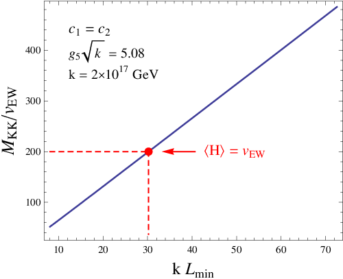
In the left panel of Fig. 2 we show as a function of . We obtain different values of by varying the localization of the fermions. For illustration purposes, we took , but the situation is similar in the more general case. We fix so that has the correct55 5 We use the RG equation with the SM field content plus one additional singlet quark with a mass of a , for reasons discussed in Section 3, to obtain the value of from . value at when the condensate has the correct value, . These two requirements uniquely fix and (for and we find ). The size of the extra-dimension, , is fixed by the minimization of the potential to be . The hierarchy between the weak and Planck scales is explained when is within of , a relatively moderate tuning. 66 6 Defining the sensitivity by [28], we obtain . As argued in [29], the fine-tuning should be obtained by comparison with the typical sensitivity, defined as an appropriate average, which in our case is . For , , and we find , which corresponds to a fine-tuning. The KK scale is then predicted to be (see right panel of Fig. 2). Interestingly, the radion is stabilized at a point where the actual coupling of the KK gluon to fermions, [see Eq. (10)], is rather close to the critical coupling . Specifically, we get
| (25) |
which gives . Notice that is closer to than the original input by a factor , which is small because , a consequence of the underlying strong dynamics. This accounts for the factor of about of additional suppression in the difference . As a result, a relatively large hierarchy between and is predicted:
| (26) |
as shown on the right panel of Fig. 2. In that figure we also marked the point where , which is associated with a KK scale (and ). We stress that the hierarchy between and of about 200 requires only a moderate tuning, so that there is essentially no little hierarchy problem. This is a consequence of the radion stabilization mechanism that relaxes to a point where is driven very close to the critical value. This also implies that generically only the fermions closest to the IR brane, which have the strongest couplings to the first-level KK gluon, will condense. Other fermions which are somewhat further away from the IR brane will have subcritical couplings. This is also true for the fermion KK modes, which have couplings to the KK gluons that are smaller than those of the lightest fermion modes (see comments in the last paragraph of Subsection 2.1).
2.5 Scales: Improved Analysis
To estimate more precisely the renormalized fermion Yukawa coupling and the Higgs quartic coupling , hence the Higgs boson mass, at a low energy scale , we include the SM gauge couplings and Higgs self-interactions into the renormalization group (RG) equations for and . 77 7 The Higgs mass parameter also receives quadratically divergent contributions from gauge boson loops, which should be added to Eq. (13). Since these couplings are perturbative, this shift changes the value of the critical coupling (defined by the vanishing of the Higgs mass parameter) only slightly. As mentioned before, the loop contribution due to the Higgs self-interactions is also small in the large limit. The details of the minimization of the radion potential are expected to change only slightly as a result of these effects. At one loop order these are [11]
| (27) | |||||
| (28) |
while the SM gauge couplings satisfy
| (29) |
with
| (30) |
Here we introduced and to take into account additional particles beyond the standard model, which will be discussed in a realistic model in Section 3. We will choose for TeV and for TeV, while for TeV and for TeV. This corresponds to having one additional Higgs doublet at TeV and one additional top quark-like fermion at TeV. To solve the RG equations, we use the “compositeness conditions” and at the scale [11], which corresponds to having vanishing Higgs kinetic term and quartic coupling at the compositeness scale, TeV. In the following numerical studies the SM gauge couplings at are taken from the PDG [30], while their experimental errors are neglected since they are expected to be small compared to the theoretical uncertainties.


In Fig. 3, we show the fermion and the Higgs boson masses as functions of the energy scale , that follow from integration of Eqs. (27) and (28). We use the mass-shell condition to define the physical mass. To estimate the error in our perturbative calculation of a strongly coupled theory, we report two boundary conditions for . One is as shown in the solid (blue) line, while the other is as shown in the dotted (orange) line. In this way, we find a fermion mass of GeV, while the Higgs boson mass is GeV. The actual masses of the new fermion and the new Higgs doublet are not important for the numerical solutions of the RG equations. If we neglect the effects from the new particle’s contributions by choosing for all scales in Eq. (29), the final values for and are only changed by around GeV, and hence contribute negligibly to the errors of and . However, the RG improved masses of the new fermion and Higgs doublet are relevant to study the phenomenological consequences of this scenario.
2.6 Corrections to the Condensate-Induced Radion Potential
We studied in the previous subsections the physical consequences of having the interbrane separation dynamically fixed through a potential arising as a result of fermion-anti fermion condensation. Whether the condensate forms or not depends on , thus leading to a non-trivial connection between the condensation scale (which we call ) and the KK scale , with and . Interestingly, a dynamically induced little hierarchy between and arises (see Subsection 2.4). The relevant quantities that enter in this argument are and , which we can think of as parametrizing the strength of the 4-fermion interactions in a large expansion, according to . This strength should be compared to a critical value , above which the fermion condensation occurs. In a large approximation, is given by . For finite one might expect that there is still a critical value, although it may differ from the large result by order one. Determining the precise at finite would require a fully non-perturbative analysis. Absent this, we take the attitude that the large result may be a useful guide even for . Notice that in this case, , a value that is in the ballpark of , and is at the heart of the mechanism we have presented. The effects of fermion localization give a freedom that accounts for the fact that these two quantities are not numerically identical. The important point is that the precise value of was not essential in our analysis (as long as it is not too far from the large result).
Besides the large approximation, that gives some analytic control to explore our stabilization mechanism, we also used in the quantitative analysis of the previous subsections the tree-level results for the functions and , as given in Eqs. (7) and (8). Given that the matching at the KK scale between the 4D effective theory and the 5D model involves strongly coupled physics,88 8 We argue in Apendix A that this strong coupling should not be interpreted as a signal of the breakdown of the 5D description. The 5D description breaks down at a scale somewhat larger than . one can expect that the non-perturbative functions and can differ by order one from the tree-level values, even in the large approximation.99 9 We thank K. Agashe for discussions on this point. Notice that the analysis of the relation between scales given in Subsection 2.4 is phrased in terms of , and . In particular, we only use that where the large values arise from , thus reflecting the strength of the coupling between fermion zero-modes and the KK gluon. It is also important that and be positive, which is indeed the case at tree-level.
The lesson is that provided the fully non-perturbative values of and are of the same order and have the same sign as the tree-level result, the qualitative picture discussed above applies (notice that the sign of corresponds to the statement that the 4-fermion channel is attractive). Again, absent a fully non-perturbative analysis, we cannot assess whether this assumption is indeed fulfilled, but we find it extremely interesting that a little hierarchy can be dynamically induced under this seemingly mild assumption. In particular, one might expect the hierarchy between and to be of order [setting in Eq. (26), roughly a 10% tuning of microscopic parameters]. In order to get a more quantitative estimate of the non-perturbative effects on the radion stabilization, one can test how much changes (keeping and fixed) if change by a factor of order one compared to the tree-level values (our intention is only to roughly mimic possible non-perturbative effects, and we do not change here the and dependence given by and ). For instance, if one finds , while for one finds [there is slightly less sensitivity to corrections to : as it varies from to , varies from to ]. We infer that a KK scale of a few tens of TeV may be expected, as already suggested by the tree-level matching. We also note that the above examples require the same tuning of microscopic parameters that was found in Subsection 2.4. It is important to recall that given the values of and , the radion potential has the striking property that the ratio of to is quite insensitive to the only mass scale in the Lagrangian, namely (as we will show later, only the radion mass and couplings are sensitive to this high scale).
Also to be addressed are the effects of other contributions to the radion potential, not associated with the condensation. For instance, we neglected above the -dependence of in Eq. (9). This dependence contributes to the calculable Casimir energy contribution [31, 32] and should be taken into account. It was shown in Ref. [32] that the contribution from localized fermions is exponentially smaller than the contribution due to gauge fields (or other fields with approximately flat zero-modes). The latter takes the form , where is the number of degrees of freedom of the gauge fields in the SM plus the graviton contribution, and is a calculable function that depends on the localized kinetic terms. For and , one has . This should be compared to the value of the potential Eq. (20) at its minimum, which using Eq. (21) can be written as . Thus, it appears that a suppression is required, or else the dynamically induced little hierarchy would be questionable. In fact, for gauge fields with negligible brane kinetic terms one has (i.e. the branes are attracted to each other), and the minimum of in Eq. (20) is destabilized. However, depends on the brane kinetic terms and can easily be positive, in which case the radion potential has a minimum and the connection to EWSB is maintained (the physics of brane-localized kinetic terms in regards to Casimir energies was first pointed out for the flat case in [23]). For instance, an IR localized kinetic term with a coefficient () leads to (). Minimizing , and requiring that and have the observed values, as in the previous sections, one finds that (). The above remarks also show that there is a value of the brane kinetic term that makes the one-loop Casimir energy vanish.1010 10 We thank H. Davoudiasl for discussions on this scenario. In particular, leads to . In fact, even for –where the Casimir contribution at the “unperturbed” minimum is somewhat larger than the condensate potential– a minimization of the potential including both the Casimir and the condensation contributions leads to . The non-trivial minimum arises from the condensation, and the link between and , as well as the little hierarchy, survive.
We also mention a second way to suppress the Casimir contribution. The important observation is that the leading order Casimir effect [], at one-loop order, depends only on the particle content. Also, the contribution can be positive or negative depending on the statistics (as well as on the b.c.’s). We can therefore simply add a number of “inert” 5D fermions with that match the degrees of freedom of the SM gauge fields. Writing a small IR localized Majorana mass so as to avoid an additional fermionic zero-mode, the Casimir effects due to the gauge fields and the additional fermions cancel at leading order, and the remnant is of order , where is the mass of the lightest fermion state in the KK tower,1111 11 In the case of the and , is the mass splitting between the fermion and the gauge bosons. is a calculable numerical factor, and we used on the r.h.s. For , this is comparable to the potential from condensation for , and becomes rapidly negligible for smaller (note that any choice for is technically natural). We are taking advantage here of the fact that the one-loop Casimir energy is independent of the interactions of the particles involved and is sensitive only to the spectrum. This is no longer true at two-loop order. Since for such light fermions one needs their couplings to the SM to be sufficiently small that they have escaped detection (they could even be completely ‘‘inert’’1212 12 If, on the other hand, the new fermions interact with matter like gauginos, there are cancellations that make the two-loop Casimir contribution negligible compared to the potential from the condensate. In this case, the (long-lived) “gluinos” would have to be sufficiently heavy to have escaped detection, probably [33, 34]. The one-loop Casimir contribution discussed above is then larger than the radion potential from condensation, but it does not necessarily wipe out the minimum, nor the connection between and .), there is no cancellation between the fermions and gauge boson contributions to the Casimir energy at two loops. We expect the size of the net effect to be of order for some calculable , where is the QCD coupling. We have checked that for , and there is a minimum of the combined Casimir and condensation potential, with . It is quite possible that this mild suppression of can be easily achieved without fine-tuning, either as a result of small factors arising in the detailed two-loop computation, or due to the presence of IR brane-localized kinetic terms, as suggested by the one-loop result.
Finally, there are non-calculable contributions to the radion potential that, through the brane tensions, are sensitive to the UV completion of the 5D theory. Up to a constant, radion-independent term (that depends on the UV brane tension, , and should be adjusted to have vanishing 4D cosmological constant), the total radion potential takes the form
| (31) |
where the non-calculable contribution is parametrized by a free parameter , is the calculable Casimir contribution discussed above, and is the contribution from fermion condensation, Eq. (20). 1313 13 There can also be other, subdominant contributions, for instance associated with the QCD phase transition, that we neglect. Ref. [32] showed that a minimum with can arise from the first two terms in Eq. (31), provided one has (this can be achieved by adjusting the renormalized IR brane tension). In this case it would still be possible to generate a non-trivial condensate if the fermion zero-modes are sufficiently localized towards the IR brane, but the close connection between radion stabilization and the condensate (to be identified with the EWSB scale) would be lost. If, on the other hand, is more suppressed, a minimum can instead arise from the last two terms in Eq. (31).1414 14 The Casimir contribution is not essential for the existence of the minimum, and could also be suppressed, as discussed above. Note that assuming a suppressed would correspond to imposing . This latter relation is similar to the one required in the original Randall-Sundrum proposal [21]. However, a suppressed within the present setup would not only stabilize the distance between the two branes, but also establish a connection with the condensate. In this work we have assumed that the non-calculable part is sufficiently suppressed, for instance by a careful choice of the IR brane tension, and hence a little hierarchy between and is induced.
As a last technical remark, we note that since the potential at the minimum is of order the EW scale and much smaller than , we expect the gravitational backreaction on the warped background to be small.
3 The Planck and EW Scales from a Top Seesaw
Having discussed the mechanism for condensation and radion stabilization in Section 2, we now turn our attention to a realistic implementation where the above condensation mechanism is responsible for EW symmetry breaking and the generation of all SM fermion masses. The fermions that condense must then carry quantum numbers. One possibility is to consider a fourth generation as done recently in Ref. [17]. This leads to a Higgs mass of order a TeV, and a fourth generation fermion with a mass in the several hundred GeV range. The light fermion masses can be generated from local 4-fermion operators suppressed by the cutoff scale [see Eq. (74) below], as discussed in Subsection 3.3 below. However, such effects are naturally suppressed, and can hardly be expected to generate the top quark mass (see Subsection 3.3 and Appendix A). We therefore consider a scenario where the top quark takes an active role in the condensation mechanism. The EW scale is then closely connected to top condensation [11]. As we will see, our setup leads naturally to a Top Seesaw [12] structure, so that a top quark parametrically lighter than the Higgs can be easily accommodated.
3.1 The Model
In more detail, the SM model is embedded into 5D fields propagating on the background of Eq. (1) as follows. We concentrate on the “top sector”, which arises from an doublet 5D fermion, , with hypercharge 1/3, plus two singlet 5D fermions, and , with hypercharge 4/3.1515 15 In spite of the notation, these fields should not be identified with the fields of the toy model of Subsection 2.1. This setup has exactly one additional singlet compared to the standard minimal construction.1616 16 There is no corresponding enlargement of the field content in the first two generations. In summary, we simply take the 5D SM field content without the Higgs field and add a single 5D fermion with the quantum numbers of the RH top quark. A Chern-Simons term to cancel anomalies resulting from the compactification needs to be added [15], but it has no impact on the physics we are interested in. The boundary conditions are chosen so that has a LH zero-mode, . Since and have the same quantum numbers, we can write a general two by two 5D Dirac mass matrix for them. Such a mass matrix can always be diagonalized, but the boundary conditions in the basis where the 5D mass matrix is diagonal need not be of the simple or type for the two individual fields. Rather, one should allow for general linear combinations of the fields with the same quantum numbers to be assigned Neumann or Dirichlet boundary conditions. From now on, we will define and as Dirac mass eigenstates with Dirac masses written as and respectively, while the Dirac mass associated with the doublet is written as . The boundary conditions for the singlets are described in more detail below.
We choose one linear combination of and to have a RH zero-mode, while the orthogonal linear combination has an ultralight Dirac KK mode. The low-energy (i.e. below the KK scale) singlet fermions are denoted by , and . In general, lives in both RH 5D fermions, and , as does the ultralight Dirac KK mode, . The KK decomposition in the RH sector reads
| (32) |
where represent higher KK modes, and , are the wavefunction profiles for and , respectively. The “misalignment” between the boundary conditions and the general Dirac mass matrix for and is parametrized by an angle . We require to obey boundary conditions, so that it contains the zero-mode , while the orthogonal combination is assigned boundary conditions and contains the ultralight mode .
For the zero-mode , the wavefunction profiles are
| (33) |
Here is a dimensionless parameter that normalizes the 4D fermion wavefunction according to , and is given by
| (34) |
where was defined in Eq. (3) [ and are precisely the normalization factors of the zero-modes of 5D Dirac fermions obeying boundary conditions]. For , the solutions for the wavefunction profiles of the ultralight KK mode, , are approximately
| (35) |
where the approximation is very good even for ’s far from the IR brane. Again the wavefunction of is properly normalized here. The ultralight Dirac mass, that marries the and fields, is
| (36) |
This formula is valid for less than and when and are not too close to each other. It shows the Dirac mass to be exponentially smaller than . For , the ultralight mode arises purely from , and has a mass .
The couplings of the lightest KK gluon to the RH 4D fermions can be read from the 5D fermion covariant kinetic terms after replacing them by their KK decomposition, Eq. (32), as well as the gluon one. Noticing that and are proportional to the same exponential function, these couplings take the form
where is defined exactly as in Eq. (5) (i.e. as the coupling of the first KK gluon to a generic fermion with b.c.’s and localization parameter ). The above two matrices can be diagonalized by the same rotation matrix. Changing the RH chiral fermions basis to a new basis and , so that the fermion couplings to the first KK gluon are diagonal, we have the simple result
with the mixing angle
| (55) |
Effectively, and behave like RH zero-modes of two non-mixing Dirac fermions with localization parameters and . They couple to the LH light fermion with 4D Dirac masses, and , respectively, where is given in Eq. (36). We notice, for future reference, that the normalization factor in Eq. (34) can be variously expressed as
| (56) |
so that the wavefunction profiles of Eqs. (33) and (35) can be simply written in terms of the fundamental zero-mode wavefunctions of Eq. (2) as
| (57) |
The wavefunction of is obtained from using the equation of motion. Decomposing the 5D left-handed field as
| (58) |
and considering the region , we have
| (59) |
where the normalization factors were defined in Eq. (34). The coupling of to the first KK gluon, which we call , can be calculated simply by substituting the wave function profiles and into Eq.(5) and summing them together. As one can see, for the parameter range of interest, , the LH part of the Dirac fermion is localized close to the UV brane. As a consequence, is suppressed compared to and . More importantly, it has the opposite sign to and , a fact that will be relevant in the following.
3.2 EWSB, Radion Stabilization and the Top Mass
It is now simple to study the low-energy theory that describes the light fermions, , , and . The most important effects due to the heavy physics are the 4-fermion interactions that are induced by integrating out the KK gluons at tree-level. These lead to the breaking of the EW symmetry and the stabilization of the radion along the lines discussed in Section 2. The top mass can also be easily accommodated via a top seesaw. After Fierz rearrangement, the 4-fermion operators are
| (60) |
where is the KK gluon mass, and , , , . The analytical dependence of these coupling on can be obtained from Eq. (10), with
| (61) |
Here and are the and 5D gauge couplings, respectively, and the ’s are the appropriate hypercharges, with and . There is no contribution from the interactions since all terms in Eq. (60) involve the singlets or . For and , Eqs. (7) and (8) can be used, since they apply for fermions localized near the IR brane. However, as mentioned at the end of the previous subsection, one finds that has the opposite sign to and , so that and are negative.1717 17 For a fermion zero-mode with localization parameter (localized near the UV brane) interacting via KK gluon exchange with a second fermion with (localized near the IR brane), one has, for , with . Thus, KK gluon exchange in these channels is repulsive, and no singlet bound states can form. Bound states and condensation can only occur for and .
In order to analyze the physics of EW symmetry breaking, we introduce two scalar doublets, and , with hypercharge . In terms of these auxiliary scalar fields, the last two terms in Eq. (60) are rewritten as
| (62) |
which is understood to hold at the KK scale, . We do not write the four fermion operators involving since they do not lead to scalar bound states, nor condensation. At lower scales the scalar fields and become dynamical and, depending on the strength of their interactions with the fermions, their squared masses can become negative, thus triggering the condensation. The induced scalar kinetic terms, quartic couplings and mass renormalizations can be obtained by RG evolution. The RG equations receive contributions from the Yukawa couplings exhibited in Eq. (62), as well as from the gauge interactions and the induced quartic self-interactions. At lower energies, the Lagrangian, with kinetic terms understood, takes the form
| (63) | |||||
The bars indicate renormalized parameters with all fields canonically normalized, as in Eq. (16):
| (64) |
where the ’s are the scalar wavefunction renormalization constants induced at low-energies. Here only the effects of the Yukawa interactions are shown, and the are given by Eqs. (13) replacing the appropriate Yukawa couplings. An improved analysis that takes into account the effects of the gauge and quartic couplings is straightforward. As will become clear in the following, in the case of interest to us the RG improved analysis is identical to the analysis done in Subsection 2.5.
To simplify our discussion, we consider the following region of parameter space: , 1818 18 We choose without loss of generality, since we can always relabel and to have a more negative Dirac mass for . The assumption that is more negative than the other localization parameters ensures that the condensed bound state is a doublet under the gauge group. which leads to an ordering of 4-fermion coefficients: (with and small and negative). Furthermore, we consider the case with slightly above the critical value of the NJL model [see Eq. (14)]. Due to the relaxation mechanism discussed in Subsection 2.4, generically we have below the critical value unless is accidentally extremely close to . Hence the vacuum of the potential should have , and a nonzero VEV for . For this range of parameters, only plays a role in stabilizing the radion. The radion potential is simply given by Eq. (15), changing to :
| (65) |
The analysis to determine the VEV’s of and is the same as in Subsection 2.3.
After the EW symmetry is broken by , obtains a dynamical mass by marrying with the field. Including the Dirac mass of the light KK mode , the mass terms take the form , which can be recognized as the “top seesaw” structure. We find it more useful to consider the fermion mass matrix in the original KK basis , rather than in the rotated basis that was useful in analyzing the physics of condensation. It reads
In the limit that the Dirac mass is large, , the physical top quark mass is
| (72) |
while the mass of the extra colored physical quark field is
| (73) |
In our model, we have 5 free parameters: , , , and to fit three observed quantities: , and . Since only , and enter the potential of and , through , we determine their values first by fitting and . By minimizing the potential w.r.t. and , we show in Fig. 4 the curve in the - plane corresponding to GeV. The mass of the first KK gluon is around TeV, as can be seen on the right panel of Fig. 4, and this result is stable against variations of the localization parameters that reproduce , and insensitive to the precise value of the curvature .


In these figures, GeV and are used. We also use the effective coupling , which is defined in Eq. (61) and calculated at the TeV scale by assuming the mass of the additional field to be around TeV (see Subsection 4.2). The lower value of guarantees .
Having determined as a function of from , we are left with three parameters , and to fit the top quark mass. Substituting GeV [35] and the RG improved value of GeV as discussed in Section 2.5 into Eq. (72), we see that . Then is determined as a function of and from Eq. (55) as . Finally, only two free parameters, and , are left to determine the spectrum of other particles in our model such as the heavy top quark, which is around 2 TeV to be compatible with electroweak precision observables, as discussed in Section 4.2.
The second doublet is heavier than the Higgs boson unless one fine-tunes to be extremely close to so that it is also close to . For a typical , is around 10 TeV.
3.3 Light Fermion Masses
Since the 5D theory is non-renormalizable, 5D local 4-fermion operators are anticipated to exist in the bulk, e.g.
| (74) |
where is an unknown dimensionless coefficient, and and are 5D spinors with their zero modes and representing SM fermions (one of them is an doublet, the other one a singlet). Those operators involving only the top and fields can be added to the 4-fermion interactions induced by gluon exchange discussed before. However, as argued in Appendix A, these contributions are expected to be a small correction compared to the gluon-induced ones. Hence, our analysis of the dynamical breaking of the EW symmetry, with the concomitant stabilization of the radion field, and the generation of the top mass is not expected to be affected much by such effects. Nevertheless, the local higher-dimension operators involving the other SM fermion fields would be responsible, in the present scenario, for giving rise to the remaining Yukawa interactions.1919 19 Notice that KK gluon exchange does not induce “non-diagonal” operators of the form Eq. (74). Indeed, after integrating out the fifth dimension, Eq. (74) induces the following 4-fermion interactions in the 4D effective theory:
| (75) |
where is the warped down cutoff, and are the standard model fermions (zero modes) and
with and as defined in Eqs. (2) and (3), respectively, while and are given in Eq. (57).
In order to see how the Yukawa couplings between the fields and the Higgs arise consider an operator of the form Eq. (75) together with the operator in Eq. (60). In terms of the bilinears and , we simply have
| (76) |
where and are linear combinations that “diagonalize” the above 4-fermion interactions, and , are the corresponding eigenvalues. To the extent that , we have while the mixing angle is given by . Only the second 4-fermion interaction on the r.h.s. of Eq. (76) is sufficiently strong to lead to a condensate, exactly along the lines discussed in previous sections. Describing this process by the introduction of an auxiliary scalar field , we end up with a Yukawa interaction of the form , where is the running Yukawa coupling at a scale , as discussed in Subsection 2.5. Therefore, the Yukawa coupling is
| (77) |
where in the second equality we used . This expression has a simple interpretation as a one-loop diagram obtained by an insertion of the operator Eq. (75), where the lines are closed with the Yukawa interaction discussed in Eq. (63). This one-loop diagram is quadratically divergent, and should be cutoff at the scale . Up to order one factors this gives rise to a Yukawa coupling of the order of Eq. (77). Notice that the fact that the one-loop integral is dominated by the scale suggests evaluation of at . Nevertheless, even at lower scales, [see Fig. 3] so that no significant changes of the previous estimate arising from these details are expected. Notice also that operators similar to Eq. (74) but involving instead of do not contribute to the Yukawa coupling.
It is useful to have approximate expressions for the above Yukawa couplings, taking into account the fact that and are localized close to the IR brane (since these fields are assumed to have the strongest interactions with the KK gluons, thus triggering EWSB by a bifermion condensate). For light SM fermions localized near the UV brane, we have
| (78) |
where, as discussed in the next section, , . In order to estimate the unknown coefficient we resort to NDA which, as shown at the end of Appendix A, gives , where . Taking also and , the -independent factor in Eq. (78) times evaluates to , which shows that the light fermion masses can be accommodated by an appropriate choice of .
For the bottom quark, which has [the localization parameter for the doublet], we need to take , in which case
| (79) |
For , and, for example, , with the other parameters as above, this leads to a mass . Given the uncertainties in the estimate of the unknown coefficient , we conclude that it is not implausible that the bottom mass also arises from the above 4-fermion interactions.
4 Phenomenology
Our model predicts two new particles beyond the SM model, besides a heavy Higgs boson with a mass around 500 GeV. They are a light radion field at the GeV scale and an extra colored heavy fermion with a mass in the TeV range. We will study constrains on new particle masses due to LEP bounds and electroweak precision observables, and discuss their phenomenological consequences in this scenario in turn.
4.1 The Radion
At tree-level in the 5D theory, the radion-dependent terms arise from the 5D Einstein-Hilbert action. The corresponding low-energy 4D action, with a canonically normalized radion reads [36]
| (80) |
where with and . Since the 4D Planck mass is , we have . Unless otherwise specified, we take and . Eq. (80) also contains the Higgs-radion potential of Eq. (65). As explained in previous sections, this determines dynamically and . Writing and , with , Eq. (65) leads to the Higgs/radion mass matrix:
where we used , defined , and it is understood that all the entries are evaluated at the minimum of the potential, [see Eq. (23)]. We see that, in general, there is mass mixing between the radion and the Higgs boson. However, since , the mixing angle is extremely small. For the benchmark point discussed in Section 3, with and , we have TeV, and the mixing angle is approximately which can be neglected.2020 20 Higgs/curvature mixing as first discussed in [37] would arise from a higher-dimension bulk operator in the 5D theory that involves four fermion fields and the Ricci curvature scalar, where the fermions bilinears are replaced by the effective Higgs degrees of freedom at energies below the KK scale. The resulting coefficient in the 4D theory is therefore expected to be suppressed at least by order , which makes it unlikely to be relevant for phenomenology. Therefore, the Higgs boson mass is still as determined in the improved RG analysis of Subsection 2.5, around GeV. The mass of the radion is , where the terms proportional to are subdominant and can be neglected. Note that the radion mass is of order . The denominator is related to the spontaneously broken conformal symmetry; the numerator is related to the explicit breaking of the conformal symmetry, since the electroweak scale is different from zero only when the localization parameters are away from the conformally invariant limit .
To have a better estimate of the allowed radion masses in our model, we vary the 5D curvature in the window GeV, and adjust so as to keep the 4D Planck mass unchanged. For each , we first determine the allowed values of and to have the correct , and then calculate the radion and Higgs boson masses. Since at the minimum of the potential, the mass of the radion takes the approximate form
| (87) |
where was defined in Eq. (22) and . The mass of the Higgs boson and the mass of the first KK gluon do not vary much when is varied, and they are still around 500 GeV and 35 TeV respectively. In the left panel of Fig. 5, the radion mass is shown as a function of . As can be seen, is a linear function of and is around a few GeV in the above window for . In the right panel of Fig. 5, the radion VEV is shown as a function of , and, for , is of order a few hundred TeV.


The radion field couples to ordinary matter via the energy-momentum tensor, and its couplings are inversely proportional to the scale invariance (spontaneous) symmetry breaking scale. In more detail [38],
where is a function that depends on the fermion localization parameter, and and are the QCD and QED beta functions, taking all fermions lighter than the radion into account. LEP imposes bounds on the couplings of a light scalar to gauge bosons [39]. For the radion, these couplings are controlled by the ratio , which in our case is a . This is below the current LEP upper bound on this ratio, which is about .
4.2 Electroweak Precision Constraints and Spectrum
The oblique parameters and constrain the remaining two model parameters and ( has already been determined by , is determined by , and is determined by ). The parameter in our model is much smaller than the and parameters, and is neglected in the following. In Appendix B, we give the formulas for and in our model, defined as the deviations of and from the standard model with a Higgs boson mass of GeV. The dominant contribution to comes from the heavy Higgs of mass - GeV. The heavy fermions give a smaller contribution, and we have for a wide range of choices of and . A two-parameter fit to the EW data with a reference mass of requires for , at the CL.2121 21 The fit does not include low-energy data, but the latest measurements of GeV and GeV at the Tevatron are included in the fit. We thank Jens Erler for kindly providing the fit results, which we have reproduced with good agreement using the code in [40].
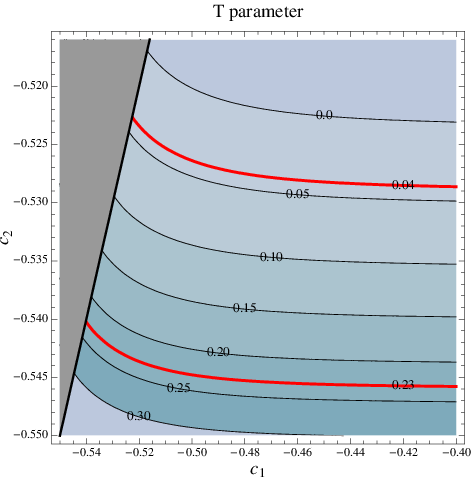
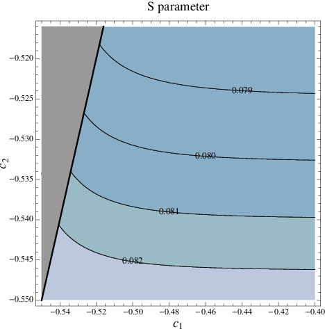
In Fig. 6, we show the allowed region of parameter space that satisfies the electroweak constraints. We impose , as discussed in Subsection 3.2. We also use GeV and GeV as described in Section 2.5. The left panel of Fig. 6 shows a contour plot of the parameter as a function of and . The curves of constant are most sensitive to and are only mildly dependent on . This is because, for fixed , the Dirac mass controls the mixing of the left-handed top quark with the fermion singlet –which dominantly determines the contribution to from the fermion loops– and is mainly controlled by . Since the GeV Higgs boson contributes to , a positive and non-negligible contribution from fermion loops is necessary to bring the parameter back to the experimentally allowed region. Therefore, there is an upper bound on the Dirac mass (via an upper limit on ). In the right panel of Fig. 6, we show a contour plot for the parameter as a function of and , showing that indeed in the region of interest (the GeV Higgs boson contributes to while contributes ). There are also tree-level contributions to the and parameters that arise when the heavy KK gauge bosons are integrated out, but for these are one order of magnitude smaller than the fermion and Higgs boson loop-level contributions, and are not included in the plots.
Notice that in our setup the doublet is extremely localized towards the IR brane, thus triggering EWSB through the condensate. As mentioned above, the KK scale is dynamically set to be about TeV, which corresponds to . This high scale allows localizing the light families close to the UV brane –so that the fermion mass hierarchies arise from wavefunction localization effects– without inducing large anomalous contributions to the coupling due to mixing with the heavy KK gauge bosons. In fact, assuming that the light fermions are localized near the UV brane, we have 2222 22 We assume that the EW breaking VEV is effectively localized on the IR brane. A more detailed analysis that takes into account the fact that the fermionic Higgs constituents have profiles that extend into the extra dimension most likely will reduce this estimate even further.
| (88) |
For , and , one finds . There is also a loop-level correction to the vertex induced by the vector-like quark through its mixing with the top quark. In the limit that is much heavier than the top quark, we have [41]
| (89) |
which gives2323 23 We thank José Santiago for pointing out a missing factor in Eq. (89) of an earlier version. for TeV (see below), GeV and . Adding the tree-level and loop-level contributions, one has , which is comparable to the current experimental bound. Moreover, the dominant contributions to and depend on the same underlying model parameters (but are essentially uncorrelated with ). Nevertheless, we have checked that the CL ellipsoid resulting from a simultaneous fit to , and , using the code in [40], results in essentially the same allowed range in as discussed above. Therefore, the additional constraints from turn out to be very mild.

The constraints from EW observables discussed above in the - plane allow us to constrain the mass of the vector-like fermion . For less than but not too close to , so that , we obtain an approximate expression for , which is almost independent of :
| (90) |
Recall that for GeV. This approximate formula for holds for and is within of the exact value. In Fig. 7, we show the mass of the field as a function of . The contribution to due to the fermion depends on the Dirac mass and the mixing with the top quark which is governed by [see Eq. (3.2)]. The dashed line corresponds to the central value GeV. The band corresponds to the variation of between 350 GeV and 400 GeV. We adjust the angle to reproduce the top mass , and also take into account its effect, through , on [see Eqs. (36) and (55), although we do not use the approximate expression (36) but instead solve the exact eigenvalue equation to obtain ]. We see that the electroweak constraints determine to be between and TeV.
4.3 Collider Phenomenology
In this section, we explore the prospects for discovery of the heavy Higgs boson and the new colored fermion at the LHC. After diagonalization of Eq. (3.2), we obtain the top and heavy fermion mass eigenstates with their masses given by Eqs. (72) and (73). As discussed above, our model has definite predictions for their masses. To simplify the notation, from now on we shall denote the fermion mass eigenstates as and . The relevant interactions of and with other particles in unitary gauge are
where are the top and electric charges and with the left- and right-handed mixing angles obtained from diagonalization of the fermion mass matrix, Eq. (3.2). The exact formula for is given in Eq. (102), but for we have the simple result . For , GeV and TeV we have . The right-handed mixing angle is for the same set of parameters. We note here that deviations of the top Yukawa coupling from its SM value are of order , which, for the above parameters, results in a decrease of about .
The Higgs boson in our model has a mass around 475 GeV, and is heavy enough to decay into a pair of gauge bosons, gauge bosons or top quarks. Taking the running of fermion masses into account, a SM Higgs of mass 475 GeV has a total width of GeV, and the branching ratios of the three main decay channels are , and , respectively [42, 43]. In our model, the changes of those branching ratios from their SM values are of order due to the deviation of the top Yukawa coupling from its SM value, and are negligible. Unlike a light Higgs, a heavy Higgs boson mainly decays to gauge bosons due to the enhancement of its decays into the longitudinal components of the gauge bosons as its mass gets larger.
At the LHC, the dominant production of the Higgs boson is through gluon fusion. The new quark , is too heavy and has too small a coupling to the Higgs boson (its mass gets only a small contribution from the EWSB) to contribute appreciably to the Higgs boson production. Compared to the Higgs boson in the SM with the same mass, the production rate from the top quark contribution is suppressed by at most a few percent due to a slightly smaller top Yukawa coupling. At next-to-next-to-leading-order in QCD, the SM cross section to produce a 475 GeV Higgs boson at the LHC is about 7 pb [44, 45, 46]. For values of the Higgs mass around , the decay is the “gold-plated” mode for discovery at the LHC [47].
We also predict a new colored fermion that mixes with the top quark and has a mass in the window to TeV. Since is much heavier than the other particles in the SM, the Goldstone boson equivalence theorem implies
| (92) |
The total width of is approximately GeV for TeV. Independently of the mass of the field, as long as it is large, it decays to with a branching ratio, and to and with an equal branching ratio of .
The strength of the single production rate is governed by , which relates to by . The single production rate is larger than the pair production rate by more than two orders of magnitude when the mass is around 2 TeV [48, 49, 50]. 2424 24 The coupling among , and in our model can be mapped to the case in [50]. Therefore, single production through the process provides the best discovery channel at the LHC. Existing studies on new top-like quarks at the LHC show that the field can be discovered up to TeV with 300 luminosity at a significance [50] by studying the decay chain . This covers a wide range of the expected values of in this scenario. Specific to our model, the decay chains and would provide interesting signal topologies for the presence of the heavy quark and Higgs boson, and deserve more careful studies at the LHC.
5 Conclusions
We have considered the intriguing possibility that there may exist a deep connection between two of the known fundamental scales in nature: the Planck and the EW scales. Our framework is based on the observation that the existence of a warped extra-dimension can provide such a deep link through the dynamical determination of the ratio between the two scales. As a byproduct, a third scale, the scale of KK resonances, is dynamically fixed in this model.
The scenario we envision is as follows: there are no fundamental scalars, and the 5D version of the SM (without a Higgs) is supplemented by a single singlet 5D fermion without zero-modes. The EW symmetry is broken as a consequence of top condensation, which results from the strong interactions associated with the lightest KK gluon resonance. In the low-energy theory there appears an effective Higgs degree of freedom with a mass of about and SM-like properties. The fact that the top mass is of order the EW scale is understood as a result of the prominent role the top plays in the breaking of the EW symmetry, as in Topcolor [18] and top seesaw [12] scenarios. Our main observation is that the physics that leads to condensation automatically induces a potential that stabilizes the distance between the UV and IR branes (described by a radion field). Thus, the large hierarchy between the Planck and EW scales is determined dynamically. Interestingly, when the radion relaxes to the minimum of the potential induced by EW symmetry breaking, the KK scale is determined to be about two orders of magnitude above the EW scale. Our analysis was performed in the large approximation, but we identified the basic ingredients behind the mechanism, which may hold beyond this approximation. Additional calculable contributions to the radion potential may be suppressed in the presence of additional fermionic degrees of freedom that need not interact with the SM fields. The non-calculable contributions to the radion potential are assumed to be suppressed in a way not necessarily related to EWSB. If this is not the case, the little hierarchy between and may not survive.
The prediction that the KK scale is parametrically larger than the electroweak scale allows the scenario to be consistent with EW precision constraints, since corrections due to the KK physics are appropriately suppressed. The negative contribution to the Peskin-Takeuchi parameter from the Higgs can be compensated by the contribution from a relatively light vector-like quark that mixes with the top quark. In particular, the mass of this new fermion is expected to be between and TeV, and should be observable at the LHC via single production for most of its expected range. A light radion field with a mass of order a few GeV is also predicted, although its observation is expected to be challenging since it couples weakly to SM matter. Summarizing, the Higgs will be accessible at the LHC with a few or less, although it will be rather difficult to distinguish it from a SM Higgs. Deviations from the SM in the coupling of order , which would induce small variations in the gluon fusion Higgs production and in the Higgs branching fractions, will be most likely beyond the LHC sensitivity given theoretical and experimental uncertainties. This small variation could be probed at a future lepton collider. The new light vector-like fermion with mass in the range will require LHC integrated luminosities above , and would be the first direct new physics signal of this scenario beyond the SM.
It is perhaps somewhat disappointing that the physics ultimately responsible for the radion stabilization mechanism (the KK states) lies beyond the reach of the LHC. On the other hand, the feature that the KK states are rather heavy, might be counted as a success from the point of view of EW precision tests. Notice, however, that the discovery of a vector-like quark with a mass in the TeV range might be taken as indication for the existence of an extra dimension that plays a role in EWSB. A Higgs could suggest the presence of strong dynamics. Our scenario would represent an example of a theory that defies the commonly held expectations that new TeV-scale particles responsible for the cancellation of quadratic divergences in the Higgs boson mass parameter should be present. In the model described in this paper, both the loop contributions to the Higgs mass parameter and the “bare” Higgs mass are of order the KK scale. But the dynamics of our scenario, through their radion dependence, leads to a cancellation between these two contributions, resulting in a Higgs mass of order the electroweak scale.
We also stress that localization of fields in the extra-dimension plays a unifying role in this scenario. The fermions that condense are the two most closely localized near the IR brane. The radion stabilization mechanism drives their 4-fermion interaction strength down, leaving it slightly above criticality and triggering condensation. On the other hand, 4-fermion couplings associated with other fermions not so close to the IR brane are reduced, generically lie below the critical value and do not lead to additional bi-fermion condensates. This makes our scenario distinct from previous extra-dimensional realizations of EWSB via fermion-anti fermion condensation [15, 16]. The effective Higgs degree of freedom can be thought as being localized near the IR brane, in the sense that its fermion constituents are. In addition, we showed how all fermion masses other than the top mass can arise from “fundamental” 4-fermion interactions. This results in a scenario where the observed fermion mass hierarchies and flavor structure can be obtained from the localization of the fermions along the extra-dimension, realizing the picture of flavor from anarchy. It is interesting that the same higher-dimensional mechanism of fermion localization can be at the heart of the physics of flavor and EWSB. We find it remarkable that this simple setup can provide rather non-trivial connections among the physics of gravity, EWSB and flavor.
Acknowledgements
We thank Thomas Appelquist, Bogdan Dobrescu, Christopher Hill, Markus Luty and Carlos Wagner for useful comments, and in particular Bill Bardeen for illuminating discussions. E.P. wishes to thank the Fermilab Theory Group for hospitality during various stages of this work. Fermilab is operated by Fermi Research Alliance, LLC under contract no. DE-AC02-07CH11359 with the United States Department of Energy. E.P. was supported by DOE under contract DE-FG02-92ER-40699.
Appendix A Validity of the Effective Theory
In the main text we analyzed the low-energy physics associated with the 4-fermion interactions that arise when the KK gluons are integrated out at tree-level. In order for the condensate to form, this coupling needs to be supercritical, hence in the strong-coupling regime. One might then wonder about the reliability of the above results, in particular as regards the radion potential. In this appendix we clarify the precise sense in which the theory is strongly coupled, and argue that the 5D UV cutoff is 10 times the curvature scale and is essentially independent of the fermion zero-mode localization paramter .
We start by discussing the relation between the two scales and , and arguing that they are indeed distinct, with , in spite of the strong coupling that participates in the condensation mechanism. The important point to realize is that the supercritical coupling, Eq. (10), is obtained by means of localizing the fermion zero-modes very close to the IR brane, not by increasing the 5D gauge coupling .2525 25 In fact, if we identify with the gauge coupling associated with the SM strong interactions, is of similar size as in standard RS scenarios with bulk fields (or slightly smaller since one has to match to the 4D gauge coupling at a KK scale of order tens of TeV, as opposed to a few TeV.) Furthermore, the localization affects almost exclusively the fermion zero-mode. The fermion KK modes become somewhat heavier when the zero mode is localized closer to the IR brane, while their couplings are rather insensitive to the value of . For instance, if we concentrate on the physics at the IR brane, where couplings are largest, the KK mode wavefunctions obey , essentially independent of . Recall that, in the KK picture, the large values of these wavefunctions are precisely the reason that the KK modes are more strongly coupled than the zero mode. What is happening as becomes more negative is that the couplings of the zero mode increase roughly like , 2626 26 This formula is a reasonable approximation for . As , the coupling turns to . and can become as large as those of the KK modes. It follows that only those observables that are IR dominated, hence potentially sensitive to the fermion zero-mode, can be sensitive to the value of . On the contrary, observables that are UV dominated do not depend on . This observation will be important when estimating the unknown coefficients of various operators in the underlying 5D theory.
It is instructive to understand the above statements in terms of the fermion propagator in the mixed position/momentum space representation. Considering a fermion with a LH zero-mode, the propagator describing the zero-mode tower takes the form , where is the 4-momentum. The exact result for this propagator is given in Eq. (24) of Ref. [51].2727 27 We define the propagators as the inverse of the relevant quadratic operator, , including warp factors: . The mixed position/momentum space Feynman rules for the vertices contain also the appropriate warp factors. For instance, for the fermion gauge interactions, one should use , for . When considering UV sensitive loops, only the case with is relevant (non-local effects have an associated Yukawa suppression that ensures they are finite). For illustration purposes we concentrate on the physics near the IR brane, so that . In this case, one finds in Euclidean space,
| (93) |
where , and the first approximation is excellent for and , which contains the region of interest. We see, as indicated by the arrow, that as soon as becomes a few times larger than , the propagator attains its 5D behavior, which is not only independent of but, as expected, is also identical to the flat space result (the warp factors simply combine to redshift the mass scales appropriately). Thus, UV sensitive loops can be estimated as in flat space and are independent of the strong interactions associated with the zero mode when it is localized near the IR brane.
With the above understanding, we proceed to estimate the cutoff of the 5D theory. We define the scale as the lowest scale where an interaction gets strong, understood as the scale where the loop expansion breaks down (adding a loop to a diagram by using the interaction in question does not lead to a suppression). For instance, the fermion one loop contribution to the gluon self-energy is
where is the number of flavors [in the fundamental representation of ], and we used that gauge invariance requires the result to be proportional to . In the second line we used the fact that the propagator decays exponentially over distances of order , and that the momentum integral is dominated by , so that is required to be within of . Using Eq. (93) for , removing the trivial warp factor, and using the indicated cutoff (which corresponds to a truncation of the KK sums), we have . Using this result, the parenthesis in the above diagram evaluates to . Notice that the above careful computation using the propagator (93) leads to the same result that one would have obtained in an uncompactified 5D theory. The NDA estimate for then corresponds to
| (94) |
where is the 5D loop factor,2828 28 Although in this one-loop diagram one gets a loop factor suppression of , in general the “natural” variable in the momentum integrals is , which leads us to define the generic loop factor with an additional factor of [52]. Of course, NDA should be taken with a grain of salt at this level of precision. and we replaced to take into account the diagrams involving the self-interactions. Matching to the 4D coupling constant, , we get
| (95) |
This result holds both in flat and warped spaces. In warped space, however, we are interested in the relation between and :
| (96) |
which for and gives . If we consider the SM strong interactions with the SM field content then , and , so that . This is large enough for the propagators to attain their asymptotic 5D behavior and validates the previous analysis, in particular that divergent integrals can be estimated as in a flat, uncompactified 5D theory. We stress that this estimate is essentially independent of the strong localization of certain light fields towards the IR brane, and the validity of the 5D theory is as well justified as in other RS scenarios with SM fields in the bulk.
Having established that the cutoff is well above the KK scale, we can estimate the coefficients of various operators in the underlying 5D theory. In the main text, we considered the effects of 4-fermion operators induced at the KK scale. However, one can also write directly 4-fermion operators in the 5D theory:
| (97) |
where the ’s are arbitrary matrices and the indices run over all the fermions. These include the quark flavors as well as any additional singlets (leptons). Considering the one-loop self-renormalization of the 4-fermion interactions, and assuming that the dimensionless coefficients are all of the same order, we estimate
Comparing to the tree-level 4-fermion interaction, we see that the NDA estimate for is , where counts the number of diagrams that can contribute to the loop. The 4-fermion interaction also renormalizes the gluon self-energy considered above, e.g.
where we indicated schematically the dependence on the external momentum required by gauge invariance. Using the NDA estimate for , we see that this contribution is suppressed compared to the diagrams that do not involve the 4-fermion interaction by a factor , which is typically much smaller than one. We therefore see that the gauge interactions are expected to be stronger than the 4-fermion interactions and should be used to estimate the cutoff , as done above. It is easy to check that this picture holds at higher loop orders.
We can now estimate the size of the above 4-fermion interactions in the low-energy 4D theory:
| (98) |
where , and contains the dependence on the zero-mode wavefunctions given in Eq. (2). For the fermions that are localized near the IR brane, one has , where we took, for simplicity, a common localization parameter . Thus, this 4-fermion operator is suppressed compared to (4) by
| (99) |
where we used the leading order term for from Eq. (10), with , and the NDA estimates for , and discussed above. Using , , , this gives a suppression . The number of contributing diagrams, , depends on the type of operator we are considering. For instance, for the operators considered in Subsection 3.3 that are responsible for giving masses to the fermions other than the top: where the ’s are doublets and the ’s are singlets, we typically have [the first term counts quarks, three doublets and four singlets including the additional field, the second counts the leptons]. We therefore see that these incalculable effects are expected to be subdominant in regards to the physics that leads to fermion condensation. However, notice that these 4-fermion operators can be included in the analysis of condensation and radion stabilization together with those induced by KK gluon exchange. They simply correspond to adding a new (small) contribution to the -dependent function of Eq. (7), , while leaving in (8) unchanged [see the expression for above Eq. (99), or also Eq.(79)]. Thus, the mechanism described in the main text is expected to change only in small details.
Appendix B The and parameters
In this appendix we collect the formulas for the contributions to the and parameters in our model, and . These are defined as the deviation from the SM with a fixed reference Higgs mass. There are two main sources for non-zero and : one from the vector-like singlet fermion that mixes with the LH top, and a second one from the fact that the Higgs field in our model is heavier than the reference value. The latter effect gives a contribution [53]
| (100) |
where GeV is the reference Higgs boson mass, and is the weak mixing angle. The contribution due to the fermion loop is [54]
| (101) |
where , and , are short notations for and , with the mixing angle of the LH top quarks:
| (102) |
obtained by diagonalization of Eq. (3.2). Here the functions , and are defined by
| (103) | |||||
with
| (104) |
and
| (105) |
Other than , all are symmetric functions under the interchange of the variables and .
While both the Higgs and fermion loops give a positive contribution to , the contribution to from the Higgs boson is negative and can be compensated by the positive contribution due to the fermions. In our model, since TeV is much larger than the electroweak scale, we neglect the tree-level contributions to the and parameters that arise when the KK gauge bosons are integrated out. Other contributions to the parameter coming from purely LH 4-fermion interactions, as discussed in [55], are negligible.
References
- [1] S. Weinberg, Phys. Rev. D 13, 974 (1976).
- [2] L. Susskind, Phys. Rev. D 20, 2619 (1979).
- [3] E. Eichten and K. D. Lane, Phys. Lett. B 90, 125 (1980).
- [4] S. Dimopoulos and L. Susskind, Nucl. Phys. B 155, 237 (1979).
- [5] T. Appelquist, M. Piai and R. Shrock, Phys. Rev. D 69, 015002 (2004) [arXiv:hep-ph/0308061].
- [6] Y. Nambu. Quasisupersymmetry, bootstrap symmetry breaking and fermion masses. Invited talk to appear in Proc. of 1988 Int. Workshop New Trends in Strong Coupling Gauge Theories, Nagoya, Japan, Aug 24-27, 1988.
- [7] V. A. Miransky, M. Tanabashi and K. Yamawaki, Phys. Lett. B 221, 177 (1989).
- [8] V. A. Miransky, M. Tanabashi and K. Yamawaki, Mod. Phys. Lett. A 4, 1043 (1989).
- [9] W. J. Marciano, Phys. Rev. D 41, 219 (1990).
- [10] W. J. Marciano, Phys. Rev. Lett. 62, 2793 (1989).
- [11] W. A. Bardeen, C. T. Hill and M. Lindner, Phys. Rev. D 41, 1647 (1990).
- [12] B. A. Dobrescu and C. T. Hill, Phys. Rev. Lett. 81, 2634 (1998) [arXiv:hep-ph/9712319]; R. S. Chivukula, B. A. Dobrescu, H. Georgi and C. T. Hill, Phys. Rev. D 59, 075003 (1999) [arXiv:hep-ph/9809470].
- [13] H. J. He, C. T. Hill and T. M. P. Tait, Phys. Rev. D 65, 055006 (2002) [arXiv:hep-ph/0108041].
- [14] B. A. Dobrescu, Phys. Lett. B 461, 99 (1999) [arXiv:hep-ph/9812349].
- [15] H. C. Cheng, B. A. Dobrescu and C. T. Hill, Nucl. Phys. B 589, 249 (2000) [arXiv:hep-ph/9912343].
- [16] N. Rius and V. Sanz, Phys. Rev. D 64, 075006 (2001) [arXiv:hep-ph/0103086].
- [17] G. Burdman and L. Da Rold, JHEP 0712, 086 (2007) [arXiv:0710.0623 [hep-ph]].
- [18] C. T. Hill, Phys. Lett. B 266, 419 (1991).
- [19] C. T. Hill and E. H. Simons, Phys. Rept. 381, 235 (2003) [Erratum-ibid. 390, 553 (2004)] [arXiv:hep-ph/0203079].
- [20] T. Gherghetta and A. Pomarol, Nucl. Phys. B 586, 141 (2000) [arXiv:hep-ph/0003129]. Y. Grossman and M. Neubert, Phys. Lett. B 474, 361 (2000) [arXiv:hep-ph/9912408].
- [21] L. Randall and R. Sundrum, Phys. Rev. Lett. 83, 3370 (1999) [arXiv:hep-ph/9905221].
- [22] W. D. Goldberger and M. B. Wise, Phys. Rev. Lett. 83, 4922 (1999) [arXiv:hep-ph/9907447].
- [23] E. Pontón and E. Poppitz, JHEP 0106, 019 (2001) [arXiv:hep-ph/0105021].
- [24] R. Rattazzi and A. Zaffaroni, JHEP 0104, 021 (2001) [arXiv:hep-th/0012248].
- [25] Y. Nambu and G. Jona-Lasinio, Phys. Rev. 122, 345 (1961); Phys. Rev. 124, 246 (1961).
- [26] A. Jenkins, Phys. Rev. D 69, 105007 (2004) [arXiv:hep-th/0311127].
- [27] M. S. Carena, E. Pontón, T. M. P. Tait and C. E. M. Wagner, Phys. Rev. D 67, 096006 (2003) [arXiv:hep-ph/0212307].
- [28] R. Barbieri and G. F. Giudice, Nucl. Phys. B 306, 63 (1988).
- [29] G. W. Anderson and D. J. Castaño, Phys. Lett. B 347, 300 (1995) [arXiv:hep-ph/9409419].
- [30] C. Amsler et al., Phys. Lett. B 667, 1 (2008)
- [31] W. D. Goldberger and I. Z. Rothstein, Phys. Lett. B 491, 339 (2000) [arXiv:hep-th/0007065].
- [32] J. Garriga and A. Pomarol, Phys. Lett. B 560, 91 (2003) [arXiv:hep-th/0212227].
- [33] H. Baer, K. m. Cheung and J. F. Gunion, Phys. Rev. D 59, 075002 (1999) [arXiv:hep-ph/9806361].
- [34] J. L. Hewett, B. Lillie, M. Masip and T. G. Rizzo, JHEP 0409, 070 (2004) [arXiv:hep-ph/0408248].
- [35] E. .W. Varnes, Plenary talk, 34th International Conference on High-Energy Physics (ICHEP), 2008.
- [36] W. D. Goldberger and M. B. Wise, Phys. Lett. B 475, 275 (2000) [arXiv:hep-ph/9911457].
- [37] G. F. Giudice, R. Rattazzi and J. D. Wells, Nucl. Phys. B 595, 250 (2001) [arXiv:hep-ph/0002178].
- [38] C. Csaki, J. Hubisz and S. J. Lee, Phys. Rev. D 76, 125015 (2007) [arXiv:0705.3844 [hep-ph]].
- [39] P. D. Acton et al. [OPAL Collaboration], Phys. Lett. B 268, 122 (1991).
- [40] Z. Han, Phys. Rev. D 73, 015005 (2006) [arXiv:hep-ph/0510125].
- [41] M. S. Carena, E. Pontón, J. Santiago and C. E. M. Wagner, Phys. Rev. D 76, 035006 (2007) [arXiv:hep-ph/0701055].
- [42] A. Djouadi, M. Spira and P. M. Zerwas, Z. Phys. C 70, 427 (1996) [arXiv:hep-ph/9511344].
- [43] A. Djouadi, J. Kalinowski and M. Spira, Comput. Phys. Commun. 108, 56 (1998) [arXiv:hep-ph/9704448].
- [44] S. Catani, D. de Florian, M. Grazzini and P. Nason, JHEP 0307, 028 (2003) [arXiv:hep-ph/0306211].
- [45] M. S. Carena and H. E. Haber, Prog. Part. Nucl. Phys. 50, 63 (2003) [arXiv:hep-ph/0208209].
- [46] A. Djouadi, Phys. Rept. 457, 1 (2008) [arXiv:hep-ph/0503172].
- [47] CMS Technical Design Report, http://cmsdoc.cern.ch/cms/cpt/tdr/
- [48] T. Han, H. E. Logan, B. McElrath and L. T. Wang, Phys. Rev. D 67, 095004 (2003) [arXiv:hep-ph/0301040].
- [49] M. Perelstein, M. E. Peskin and A. Pierce, Phys. Rev. D 69, 075002 (2004) [arXiv:hep-ph/0310039].
- [50] G. Azuelos et al., Eur. Phys. J. C 39S2, 13 (2005) [arXiv:hep-ph/0402037].
- [51] M. S. Carena, A. Delgado, E. Pontón, T. M. P. Tait and C. E. M. Wagner, Phys. Rev. D 71, 015010 (2005) [arXiv:hep-ph/0410344].
- [52] Z. Chacko, M. A. Luty and E. Pontón, JHEP 0007, 036 (2000) [arXiv:hep-ph/9909248].
- [53] M. E. Peskin and T. Takeuchi, Phys. Rev. D 46, 381 (1992).
- [54] L. Lavoura and J. P. Silva, Phys. Rev. D 47, 1117 (1993).
- [55] R. S. Chivukula and H. Georgi, Phys. Rev. D 58, 075004 (1998) [arXiv:hep-ph/9805478].