跳到论文正文
W Papers独立论文阅读器 arXiv:0809.1580 论文正文 计算阅读时间 · 0%
引用这篇论文根据当前论文元数据生成,正式投稿前建议核对。


License: arXiv.org perpetual non-exclusive license
arXiv:0809.1580v2 [hep-ph] 12 Sep 2008

MAN/HEP/2008/23

arXiv:0809.1580
September 2008

The 1-Loop Effective Potential in Non-Linear Gauges
Lisa P. Alexander and Apostolos Pilaftsis
School of Physics and Astronomy, University of Manchester,
Manchester M13 9PL, United Kingdom

ABSTRACT

We calculate the 1-loop effective potential of an Abelian Higgs model within the Rξ/σR_{\xi/\sigma} class of non-linear gauges that preserves the Higgs-boson low-energy theorem. The Rξ/σR_{\xi/\sigma} gauge involves two gauge-fixing parameters ξ\xi and σ\sigma, and is a renormalizable extension of the Feynman–’t Hooft RξR_{\xi} set of gauges beyond the 1-loop level. By taking consistently into account Goldstone–gauge-boson mixing effects, we show how the 1-loop effective potential evaluated at its extrema is independent of both ξ\xi and σ\sigma, in agreement with the Nielsen identity. The 1-loop constant and wavefunction renormalizations are presented within this general Rξ/σR_{\xi/\sigma} class of non-linear gauges.

1 Introduction

In quantum field theory, the effective potential [1] plays an important role. It carries precious information about the vacuum structure of a given model [2, 3], and determines its stability under quantum fluctuations. The effective potential constitutes a useful field-theoretic tool for studying the dynamics of inflationary cosmology [4] and for investigating the order of the phase transition at finite temperatures [5]. Conventionally, the effective potential is denoted as Veff​(ϕ)V_{\rm eff}(\phi) and is a functional of all classical fields involved in the theory that are collectively represented here by ϕ\phi.

An important property of the effective potential Veff​(ϕ)V_{\rm eff}(\phi) is its independence on the gauge-fixing parameter, e.g. ξ\xi, when evaluated for classical field values ϕ\phi that extremize Veff​(ϕ)V_{\rm eff}(\phi). In particular, the minimum of the effective potential Veff​(ϕmin)V_{\rm eff}(\phi_{\rm min}) corresponds to a physical quantity, that is the energy density of the vacuum. Therefore, the gauge independence of Veff​(ϕmin)V_{\rm eff}(\phi_{\rm min}) is only a manifestation of this fact. Formally, the gauge dependence of one-particle irreducible (1PI) nn-point correlation functions I​Γϕn{\rm I}\hskip-1.9919pt\Gamma_{\phi^{n}}, which involve a number nn of external ϕ\phi fields, is governed by a functional differential equation, the so-called Nielsen identity (NI) [6]. The NI relates the explicit gauge dependence of the effective action I​Γ​[ϕ,ξ]{\rm I}\hskip-1.9919pt\Gamma[\phi,\xi] to a non-linear sum of the functional derivatives δ​I​Γ/δ​ϕ\delta{\rm I}\hskip-1.9919pt\Gamma/\delta\phi for all fields ϕ\phi that carry non-zero charges under the gauge group. Evidently, at the extremal points where δ​I​Γ/δ​ϕ=0\delta{\rm I}\hskip-1.9919pt\Gamma/\delta\phi=0, both the effective action and the resulting effective potential are gauge invariant.

In a gauge theory with spontaneous symmetry breaking (SSB), as the one that we will be considering here, one has to specify the gauge-fixing (GF) scheme in order to eliminate the unphysical degrees of freedom from the gauge fields. One of the frequently discussed GF schemes in the literature is the Feynman–’t Hooft RξR_{\xi} set of linear gauges, which may be described by the Lagrangian term

ℒGFRξ=12​ξ​(∂μAμ+12​ξ​g​v​G)2,{\cal L}_{\rm GF}^{R_{\xi}}\ =\ \frac{1}{2\xi}\bigg(\partial_{\mu}A^{\mu}\>+\>\frac{1}{2}\;\xi gvG\,\bigg)^{2}\;, (1.1)

where vv is the vacuum expectation value (VEV) of a complex field Φ\Phi. The GF choice (1.1) has the virtue that the mixing between the gauge field AμA^{\mu} and its associated would-be Goldstone boson GG is absent at the tree-level, thereby simplifying enormously calculations. However, as we will see here, quantum effects spoil this nice property beyond the 1-loop level.

Another disadvantage of the RξR_{\xi} set of gauges is that 1-loop effects mediated by gauge interactions [7] violate the so-called Higgs-boson low-energy theorem (HLET) [8, 9], as expressed by the simple relation:

I​ΓHn+1=∂I​ΓHn∂v,{\rm I}\hskip-1.9919pt\Gamma_{H^{n+1}}\ =\ \frac{\partial{\rm I}\hskip-1.9919pt\Gamma_{H^{n}}}{\partial v}\;, (1.2)

where HH is the radial quantum excitation of Φ\Phi, more commonly known as the Higgs boson. Note that the additional Higgs field HH in I​ΓHn+1{\rm I}\hskip-1.9919pt\Gamma_{H^{n+1}} occuring on the LHS of (1.2) carries no momentum. The violation of the HLET (1.2) is a consequence of an explicitly breaking of a dilatational or translational symmetry that governs the gauge-invariant part of the Lagrangian. Specifically, in the absence of ℒGFRξ{\cal L}_{\rm GF}^{R_{\xi}}, the Lagrangian is invariant under the translational transformation [7]

H→H+a,v→v−a,H\to H+a,\qquad v\to v-a\;, (1.3)

where aa is an arbitrary real constant. As has been shown [10], the translational symmetry (1.3) not only implies that the HLET (1.2) is manifestly satisfied, but also that the VEV vv gets only multiplicatively renormalized by the wavefunction of the Higgs field to all orders in perturbation theory.

In this paper we study the gauge dependence of the 1-loop effective potential of an Abelian Higgs model in a class Rξ/σR_{\xi/\sigma} of non-linear gauges. More explicitly, the GF Lagrangian of the Rξ/σR_{\xi/\sigma} gauges [11, 7, 10] is given by

ℒGF=−σ2​ξ​[∂μAμ+ξ​g​(H+v)​G]2.\mathcal{L}_{\rm GF}\ =\ -\;\frac{\sigma}{2\xi}\;\Big[\,\partial_{\mu}A^{\mu}\>+\>\xi g(H+v)G\,\Big]^{2}\;. (1.4)

The Rξ/σR_{\xi/\sigma} set of gauges contains two GF parameters: ξ\xi and σ\sigma. For σ=1\sigma=1, this is a non-linear realization of the Feynman--’t Hooft gauge that preserves the HLET11 1 Earlier studies have used linear gauges to study the effective potential  [12]. However, these gauges do not respect the HLET (1.2) in the RξR_{\xi}-gauge limit given by (1.1).. However, quantum corrections spoil the condition σ=1\sigma=1 beyond the 1-loop level, and a new GF parameter is required to consistently provide a renormalizable extension of the RξR_{\xi} gauges. To the best of our knowledge, there is no explicit calculation of the 1-loop effective potential in the Rξ/σR_{\xi/\sigma} set of non-linear gauges, for arbitrary ξ\xi and σ\sigma parameters. Such a calculation is not trivial, since one has to properly take into account the mixing of the gauge field with the respective would-be Goldstone boson. We then show that the 1-loop effective potential at its extrema is independent of the GF parameters ξ\xi and σ\sigma, as required by the NI. Finally, we present the 1-loop renormalization constants for couplings, masses and wavefunctions of all fields involved in the theory.

The paper is structured as follows: Section 2 briefly reviews the Abelian Higgs model and its quantization within the Rξ/σR_{\xi/\sigma} class of non-linear gauges. In the same section, we present the relevant propagator matrix that takes account of the mixing between the gauge field and the would-be Goldstone boson. In Section 3 we calculate the 1-loop effective potential for both σ=1\sigma=1 and σ≠1\sigma\neq 1. In Section 4 we extend the derivation of the NI for the two GF parameters ξ\xi and σ\sigma, and show how the 1-loop effective potential at its extrema is independent of these two parameters. In Section 5 we present the 1-loop counterterms for the field wavefunctions and for the couplings and masses for arbitrary values of ξ\xi and σ\sigma. Finally, Section 6 contains our conclusions.

2 The Abelian Higgs Model in the 𝑹𝝃/𝝈R_{\xi/\sigma} Gauge

Here we briefly review the Abelian Higgs model along with its quantization in the Rξ/σR_{\xi/\sigma} gauge [11, 10]. In detail, the Lagrangian for the Abelian Higgs model is a sum of three terms,

ℒ=ℒinv+ℒGF+ℒFP,\mathcal{L}\ =\ \mathcal{L}_{\rm inv}\>+\>\mathcal{L}_{\rm GF}\>+\>\mathcal{L}_{\rm FP}\;, (2.1)

where ℒinv\mathcal{L}_{\rm inv} is the U​(1)YU(1)_{Y} gauge-invariant part, ℒGF{\cal L}_{\rm GF} is the GF Lagrangian and ℒFP{\cal L}_{\rm FP} is the induced Faddeev–Popov (FP) Lagrangian describing the ghost interactions. The gauge-invariant part of the Lagrangian reads:

ℒinv\displaystyle\mathcal{L}_{\rm inv}\! =\displaystyle= −14Fμ​νFμ​ν+(DμΦ)∗(DμΦ)+∑i=1,2[f¯i​L(iγμDμ)fi​L+f¯i​R(iγμ∂μ)fi​R]−m2Φ∗Φ\displaystyle\!-\frac{1}{4}F^{\mu\nu}F_{\mu\nu}+(D_{\mu}\Phi)^{*}(D^{\mu}\Phi)+\sum_{i=1,2}[\bar{f}_{iL}(i\gamma^{\mu}D_{\mu})f_{iL}+\bar{f}_{iR}(i\gamma^{\mu}\partial_{\mu})f_{iR}]-m^{2}\Phi^{*}\Phi (2.2)
−λ​(Φ∗​Φ)2−2​h1​(f¯1​L​Φ​f1​R+f¯1​R​Φ∗​f1​L)−2​h2​(f¯2​L​Φ∗​f2​R+f¯2​R​Φ​f2​L),\displaystyle-\lambda(\Phi^{*}\Phi)^{2}-\sqrt{2}h_{1}(\bar{f}_{1L}\Phi f_{1R}+\bar{f}_{1R}\Phi^{*}f_{1L})-\sqrt{2}h_{2}(\bar{f}_{2L}\Phi^{*}f_{2R}+\bar{f}_{2R}\Phi f_{2L})\;,

where Fμ​ν=∂μAν−∂νAμF_{\mu\nu}=\partial_{\mu}A_{\nu}-\partial_{\nu}A_{\mu} is the U(1)Y field-strength tensor, Dμ=∂μ−igYAμD_{\mu}=\partial_{\mu}-igYA_{\mu} is the covariant derivative and Φ=12​(v+H+i​G)\Phi=\frac{1}{\sqrt{2}}(v+H+iG) is a complex field. As was mentioned in the introduction, vv is the VEV of Φ\Phi, HH is the Higgs field and GG is the would-be Goldstone boson of AμA^{\mu}. The U(1)Y quantum numbers for the various fields are YΦ=1Y_{\Phi}=1, Yf1​L=−Yf2​L=1Y_{f_{1L}}=-Y_{f_{2L}}=1 and Yf1​R=Yf2​R=0Y_{f_{1R}}=Y_{f_{2R}}=0. Note that the left-handed chiral fermions fall into a non-anomalous representation by having opposite U(1)Y charges.

The GF term in (2.1) is given by

ℒGF=ξ2​σ​B2+B​F,\mathcal{L}_{\rm GF}\ =\ \frac{\xi}{2\sigma}B^{2}\>+\>BF\;, (2.3)

where F=∂μAμ+ξ​g​(H+v)​GF=\partial_{\mu}A^{\mu}+\xi g(H+v)G is a non-linear GF function pertinent to the Rξ/σR_{\xi/\sigma} class of gauges and BB is an auxiliary field which is introduced to close the so-called Becchi–Rouet–Stora (BRS) transformations [13] off-shell. Upon integrating out the BB fields, we obtain the GF Lagrangian given in (1.4).

Finally, the FP ghost term is induced by the GF function FF as follows:

ℒFP=−c¯​(s​F)\mathcal{L}_{\rm FP}\ =\ -\bar{c}(sF) (2.4)

where c⁡(c¯)c~(\bar{c}) is the ghost (anti-ghost) field and ss is the anticommuting BRS operator [13]. The action of ss on the fields is given by

s​Aμ=∂μc,s​H=−g​c​G,s​G=g​c​(H+v),s​B= 0,s​c= 0,\displaystyle sA_{\mu}\ =\ \partial_{\mu}c,\quad sH\ =\ -gcG,\quad sG\ =\ gc(H+v),\quad sB\ =\ 0,\quad sc\ =\ 0,
s​c¯=B,s​fL=i​g​YfL​c​fL,s​f¯L=i​g​YfL​f¯L​c,s​fR= 0,s​f¯R= 0.\displaystyle s\bar{c}\ =\ B,\quad sf_{L}\ =\ igY_{f_{L}}\,cf_{L},\quad s\bar{f}_{L}\ =\ igY_{f_{L}}\bar{f}_{L}c,\quad sf_{R}\ =\ 0,\quad s\bar{f}_{R}\ =\ 0\;.\qquad (2.5)

Given these BRS transformations, the FP ghost term becomes

ℒFP=−c¯{∂2+g2ξ[(H+v)2−G2]}c.\mathcal{L}_{\rm FP}\ =\ -\bar{c}\{\partial^{2}+g^{2}\xi[(H+v)^{2}-G^{2}]\}c\;. (2.6)

In the Rξ/σR_{\xi/\sigma} gauge, the full bare Lagrangian of the Abelian Higgs model may be represented as a sum of 5 terms, i.e. ℒ=∑n=05ℒn{\cal L}=\sum_{n=0}^{5}\;{\cal L}_{n}, where the subscript nn denotes the number of the quantum fields involved. More explicitly, the individual terms of the sum are given by

ℒ0\displaystyle\mathcal{L}_{0}\! =\displaystyle= −v22​(m2+λ​v22),\displaystyle\!-\frac{v^{2}}{2}(m^{2}+\lambda\frac{v^{2}}{2})\;, (2.7)
ℒ1\displaystyle\mathcal{L}_{1}\! =\displaystyle= −v​H​(m2+λ​v2),\displaystyle\!-vH(m^{2}+\lambda v^{2})\;, (2.8)
ℒ2\displaystyle\mathcal{L}_{2}\! =\displaystyle= 12​∂μH​∂μH−12​(3​λ​v2+m2)​H2+12​∂μG​∂μG−12​[(λ+σ​ξ​g2)​v2+m2]​G2\displaystyle\!\frac{1}{2}\partial_{\mu}H\partial^{\mu}H-\frac{1}{2}(3\lambda v^{2}+m^{2})H^{2}+\frac{1}{2}\partial_{\mu}G\partial^{\mu}G-\frac{1}{2}[(\lambda+\sigma\xi g^{2})v^{2}+m^{2}]G^{2} (2.9)
−14​Fμ​ν​Fμ​ν−σ2​ξ​(∂μAμ)2+12​g2​v2​Aμ​Aμ−(σ−1)​g​v​G​(∂μAμ)+∂μc¯​∂μc\displaystyle-\frac{1}{4}F_{\mu\nu}F^{\mu\nu}-\frac{\sigma}{2\xi}(\partial_{\mu}A^{\mu})^{2}+\frac{1}{2}g^{2}v^{2}A_{\mu}A^{\mu}-(\sigma-1)gvG(\partial_{\mu}A^{\mu})+\partial_{\mu}\bar{c}\partial^{\mu}c
−ξg2v2c¯c+∑i=12f¯i(iγμ∂μ−hiv)fi,\displaystyle-\xi g^{2}v^{2}\bar{c}c+\sum_{i=1}^{2}\bar{f}_{i}(i\gamma_{\mu}\partial^{\mu}-h_{i}v)f_{i}\;,
ℒ3\displaystyle\mathcal{L}_{3}\! =\displaystyle= (σ+1)​g​Aμ​G​∂μH+(σ−1)​g​Aμ​H​∂μG+g2​v​Aμ​Aμ​H−λ​v​H3−2​ξ​g2​v​H​c¯​c\displaystyle\!(\sigma+1)gA_{\mu}G\partial^{\mu}H+(\sigma-1)gA_{\mu}H\partial^{\mu}G+g^{2}vA_{\mu}A^{\mu}H-\lambda vH^{3}-2\xi g^{2}vH\bar{c}c (2.10)
−(λ+σ​ξ​g2)​v​H​G2+∑i=12f¯i​(g​Aμ​YiL​γμ​PL−hi​H−YiL​hi​γ5​G)​fi,\displaystyle-(\lambda+\sigma\xi g^{2})vHG^{2}+\sum_{i=1}^{2}\bar{f}_{i}(gA^{\mu}Y^{L}_{i}\gamma_{\mu}P_{L}-h_{i}H-Y^{L}_{i}h_{i}\gamma_{5}G)f_{i}\;,
ℒ4\displaystyle\mathcal{L}_{4}\! =\displaystyle= 12​g2​Aμ​Aμ​H2+12​g2​Aμ​Aμ​G2−λ4​H4−12​(λ+σ​ξ​g2)​H2​G2−λ4​G4\displaystyle\!\frac{1}{2}g^{2}A_{\mu}A^{\mu}H^{2}+\frac{1}{2}g^{2}A_{\mu}A^{\mu}G^{2}-\frac{\lambda}{4}H^{4}-\frac{1}{2}(\lambda+\sigma\xi g^{2})H^{2}G^{2}-\frac{\lambda}{4}G^{4} (2.11)
−ξ​g2​H2​c¯​c+ξ​g2​G2​c¯​c.\displaystyle-\xi g^{2}H^{2}\bar{c}c+\xi g^{2}G^{2}\bar{c}c\;.

The propagators of the theory may be calculated from ℒ2{\cal L}_{2} in (2.9). We first consider the gauge sector, whose kinetic Lagrangian may be cast into the matrix form:

ℒ2G,Aμ=12​(G,Aα)​(−∂μ∂μ−mG2−(σ−1)gv∂β(σ−1)gv∂α(∂2+mA2)gα​β+(σξ−1)∂α∂β)​(GAβ).\mathcal{L}_{2}^{G,A_{\mu}}\ =\ \frac{1}{2}(G,A^{\alpha})\left(\begin{array}[]{cc}-\partial_{\mu}\partial^{\mu}-m_{G}^{2}&-(\sigma-1)gv\partial_{\beta}\\ (\sigma-1)gv\partial_{\alpha}&(\partial^{2}+m_{A}^{2})g_{\alpha\beta}+\bigg(\frac{\displaystyle\sigma}{\displaystyle\xi}-1\bigg)\,\partial_{\alpha}\partial_{\beta}\end{array}\right)\left(\begin{array}[]{c}G\\ A^{\beta}\end{array}\right)\,. (2.12)

Notice that for σ≠1\sigma\neq 1, there is a non-trivial mixing between the gauge field AμA^{\mu} and the would-be Goldstone boson GG. Inverting the matrix in (2.12), one finds the propagators in the momentum space:

DG​G​(k)\displaystyle D_{GG}(k)\! =\displaystyle= k2−(mc2/σ)(k2−m¯G2)​(k2−m¯c2),\displaystyle\!\frac{k^{2}-(m_{c}^{2}/\sigma)}{(k^{2}-\bar{m}_{G}^{2})(k^{2}-\bar{m}_{c}^{2})}\ ,
DAμ​Aν​(k)\displaystyle D_{A^{\mu}A^{\nu}}(k)\! =\displaystyle= 1k2−mA2​(−gμ​ν+kμ​kνk2)−ξσ​k2−mG2(k2−m¯G2)​(k2−m¯c2)​kμ​kνk2,\displaystyle\!\frac{1}{k^{2}-m_{A}^{2}}\left(-g^{\mu\nu}+\frac{k^{\mu}k^{\nu}}{k^{2}}\right)\ -\ \frac{\xi}{\sigma}\ \frac{k^{2}-m_{G}^{2}}{(k^{2}-\bar{m}_{G}^{2})(k^{2}-\bar{m}_{c}^{2})}\ \frac{k^{\mu}k^{\nu}}{k^{2}}\ , (2.13)
DG​Aμ​(k)\displaystyle D_{GA^{\mu}}(k)\! =\displaystyle= ξσ​i​g​v​(σ−1)​kμ(k2−m¯G2)​(k2−m¯c2),DAμ​G​(k)=−ξσ​i​g​v​(σ−1)​kμ(k2−m¯G2)​(k2−m¯c2).\displaystyle\!\frac{\xi}{\sigma}\;\frac{igv(\sigma-1)\,k^{\mu}}{(k^{2}-\bar{m}_{G}^{2})(k^{2}-\bar{m}_{c}^{2})}\ ,\qquad D_{A^{\mu}G}(k)\ =\ -\;\frac{\xi}{\sigma}\;\frac{igv(\sigma-1)\,k^{\mu}}{(k^{2}-\bar{m}_{G}^{2})(k^{2}-\bar{m}_{c}^{2})}\ .\qquad

Observe that there is a relative minus sign between the mixed propagators DG​Aμ​(k)D_{GA^{\mu}}(k) and DAμ​G​(k)D_{A^{\mu}G}(k) due to the different direction of momentum flow signified by the subscripts G​AμGA^{\mu} and Aμ​GA^{\mu}G. In (2.13), mA2=g2​v2m^{2}_{A}=g^{2}v^{2} is the physical gauge-boson mass, and m¯G2\bar{m}_{G}^{2} and m¯c2\bar{m}_{c}^{2} are unphysical parameters related to the Goldstone and ghost masses:

m¯G2\displaystyle\bar{m}_{G}^{2}\! =\displaystyle= 12​[mG2+mc2​(2−σ)]+12​[mG2+mc2​(2−σ)]2−4​mG2​mc2σ,\displaystyle\!\frac{1}{2}\;[m_{G}^{2}+m_{c}^{2}(2-\sigma)]\ +\ \frac{1}{2}\;\sqrt{[m_{G}^{2}+m_{c}^{2}(2-\sigma)]^{2}-4\frac{m_{G}^{2}m_{c}^{2}}{\sigma}}\ ,
m¯c2\displaystyle\bar{m}_{c}^{2}\! =\displaystyle= 12​[mG2+mc2​(2−σ)]−12​[mG2+mc2​(2−σ)]2−4​mG2​mc2σ,\displaystyle\!\frac{1}{2}\;[m_{G}^{2}+m_{c}^{2}(2-\sigma)]\ -\ \frac{1}{2}\;\sqrt{[m_{G}^{2}+m_{c}^{2}(2-\sigma)]^{2}-4\frac{m_{G}^{2}m_{c}^{2}}{\sigma}}\ , (2.14)

with

mG2=(λ+σ​ξ​g2)​v2+m2,mc2=ξ​g2​v2.m_{G}^{2}\ =\ (\lambda+\sigma\xi g^{2})v^{2}\>+\>m^{2}\;,\qquad m_{c}^{2}\ =\ \xi g^{2}v^{2}\;. (2.15)

In the limit σ→1\sigma\to 1, it is m¯G2→mG2\bar{m}_{G}^{2}\to m_{G}^{2} and m¯c2→mc2\bar{m}_{c}^{2}\to m_{c}^{2}. Moreover, in the same limit, we recover the more familiar expressions of the RξR_{\xi} gauge for the propagators:

DG​(k)=1k2−mG2,Δμ​ν​(k)=1k2−mA2​(−gμ​ν+(1−ξ)​kμ​kνk2−mc2),D_{G}(k)\ =\ \frac{1}{k^{2}-m_{G}^{2}},\qquad\Delta_{\mu\nu}(k)\ =\ \frac{1}{k^{2}-m_{A}^{2}}\left(-g_{\mu\nu}\>+\>(1-\xi)\frac{k_{\mu}k_{\nu}}{k^{2}-m_{c}^{2}}\right)\,, (2.16)

whereas the ghost propagator

Dc​(k)=1k2−mc2D_{c}(k)\ =\ \frac{1}{k^{2}-m_{c}^{2}} (2.17)

does not depend on the GF parameter σ\sigma; it only depends on ξ\xi through mc2m^{2}_{c}. Finally, the fermion and Higgs-boson propagators are gauge independent, given by

S1,2​(k)=1kμ​γμ−mf1,2,DH​(k)=1k2−mH2,S_{1,2}(k)\ =\ \frac{1}{k_{\mu}\gamma^{\mu}-m_{f_{1,2}}}\ ,\qquad D_{H}(k)\ =\ \frac{1}{k^{2}-m_{H}^{2}}\ , (2.18)

where

mf1,2=h1,2​v,mH2= 3​λ​v2+m2m_{f_{1,2}}\ =\ h_{1,2}v\;,\qquad m_{H}^{2}\ =\ 3\lambda v^{2}\>+\>m^{2} (2.19)

are the fermion and Higgs-boson masses, respectively.

3 The 1-Loop Effective Potential in the 𝑹𝝃/𝝈R_{\xi/\sigma} Gauge

In order to calculate the 1-loop effective potential, we use the functional expression [14, 15]:

Veff1−loop=−Cs​i​ℏ2​(Tr​ln⁡S(2)​(v)−Tr​ln⁡S(2)​(0)),V^{\mathrm{1-loop}}_{\mathrm{eff}}\ =\ -\,C_{s}\,\frac{i\hbar}{2}\ \Big({\rm Tr}\,\ln S^{(2)}(v)\>-\>{\rm Tr}\,\ln S^{(2)}(0)\,\Big)\;, (3.1)

where S(2)S^{(2)} is the second derivative of the classical action S=∫d4​x​ℒS=\int d^{4}x\;{\cal L}, i.e.

S(2)​(v)=δ2​Sδ​ϕ​(x1)​δ​ϕ​(x2)|Φ=v/2.S^{(2)}(v)\ =\ \frac{\delta^{2}\,S}{\delta\phi(x_{1})\delta\phi(x_{2})}\;\bigg|_{\Phi=v/\sqrt{2}}\ . (3.2)

In the above, ϕ\phi collectively denotes each of the quantum fields

{G,H,Aμ,c,c¯,f1,2​L,f1,2​R,f¯1,2​L,f¯1,2​R}\Big\{G,\,H,\,A^{\mu},\,c,\,\bar{c},\,f_{1,2L},\,f_{1,2R},\,\bar{f}_{1,2L},\,\bar{f}_{1,2R}\Big\}

and Cs=+1​(−1)C_{s}=+1~(-1) for one real degree of freedom that obeys the Bose–Einstein (Fermi–Dirac) statistics. Moreover, the trace Tr{\rm Tr} in (3.1) is understood to act over all space and internal degrees of freedom. For our purposes, a more convenient representation of (3.1) is

Veff1−loop=−Csi2∫01dxTr[S(2)​(v)−S(2)​(0)x⁡(S(2)​(v)−S(2)​(0))+S(2)​(0)].V^{\mathrm{1-loop}}_{\mathrm{eff}}\ =\ -\;C_{s}\ \frac{i}{2}\,\int^{1}_{0}dx\;{\rm Tr}\,\bigg[\;\frac{S^{(2)}(v)\>-\>S^{(2)}(0)}{x\left(S^{(2)}(v)\>-\>S^{(2)}(0)\right)\>+\>S^{(2)}(0)}\;\bigg]\;. (3.3)

In momentum space of n=4−2​εn=4-2\varepsilon dimension, this last expression becomes

Veff1−loop=−Csi2∫01dx∫dn​k(2​π)ntr[S(2)​(v)−S(2)​(0)x⁡(S(2)​(v)−S(2)​(0))+S(2)​(0)]V^{\mathrm{1-loop}}_{\mathrm{eff}}\ =\ -\;C_{s}\ \frac{i}{2}\,\int^{1}_{0}dx\ \int\frac{d^{n}k}{(2\pi)^{n}}\ {\rm tr}\,\bigg[\;\frac{S^{(2)}(v)\>-\>S^{(2)}(0)}{x\left(S^{(2)}(v)\>-\>S^{(2)}(0)\right)\>+\>S^{(2)}(0)}\;\bigg]\; (3.4)

and tr{\rm tr} now symbolizes the trace that should be taken only over internal degrees of freedom, e.g. over polarizations for the gauge fields and over spinor components for the fermions.

Applying now (3.4), we may calculate the 1-loop effective potential by appropriately taking into account all quantum fields ϕ\phi present in the theory. In this way, we find using dimensional regularization (DR) that for σ=1\sigma=1 [11, 10]22 2 Here we seize the opportunity to correct several typos that occurred in Eq. (A3) of [10],

Veff⁡(σ=1)1−loop\displaystyle V^{\mathrm{1-loop}}_{\mathrm{eff}(\sigma=1)}\! =\displaystyle= 164​π2[mH4(lnmH2μ¯2−32)+mG4(lnmG2μ¯2−32)+mA4(3lnmA2μ¯2−52)\displaystyle\!\frac{1}{64\pi^{2}}\Bigg[\,m_{H}^{4}\left(\ln\frac{m_{H}^{2}}{\bar{\mu}^{2}}-\frac{3}{2}\right)+m_{G}^{4}\left(\ln\frac{m_{G}^{2}}{\bar{\mu}^{2}}-\frac{3}{2}\right)+m_{A}^{4}\left(3\ln\frac{m_{A}^{2}}{\bar{\mu}^{2}}-\frac{5}{2}\right) (3.5)
−mc4​(ln⁡mc2μ¯2−32)−4​∑i=1,2mfi4​(ln⁡mfi2μ¯2−1)−m4​(2​ln⁡m2μ¯2−3)\displaystyle-m_{c}^{4}\left(\ln\frac{m_{c}^{2}}{\bar{\mu}^{2}}-\frac{3}{2}\right)-4\sum_{i=1,2}m_{f_{i}}^{4}\left(\ln\frac{m_{f_{i}}^{2}}{\bar{\mu}^{2}}-1\right)-m^{4}\left(2\ln\frac{m^{2}}{\bar{\mu}^{2}}-3\right)
−1ε(mH4+mG4+3mA4−mc4−4∑i=12mfi4−2m4)],\displaystyle-\frac{1}{\varepsilon}\left(m_{H}^{4}+m_{G}^{4}+3m_{A}^{4}-m_{c}^{4}-4\sum_{i=1}^{2}m_{f_{i}}^{4}-2m^{4}\right)\,\Bigg]\;,

where ln⁡μ¯=−γ+ln⁡4​π​μ2\ln\bar{\mu}=-\gamma+\ln 4\pi\mu^{2}, γ≈0.5772\gamma\approx 0.5772 is the Euler-Mascheroni constant and μ\mu the renormalization scale. Instead, for σ≠1\sigma\neq 1, the 1-loop effective potential in DR reads:

Veff⁡(σ≠1)1−loop\displaystyle V^{\mathrm{1-loop}}_{\mathrm{eff}(\sigma\neq 1)}\! =\displaystyle= 164​π2[mH4(lnmH2μ¯2−32)+m¯G4(lnm¯G2μ¯2−32)\displaystyle\!\frac{1}{64\pi^{2}}\Bigg[\,m_{H}^{4}\left(\ln\frac{m_{H}^{2}}{\bar{\mu}^{2}}-\frac{3}{2}\right)+\bar{m}_{G}^{4}\left(\ln\frac{\bar{m}_{G}^{2}}{\bar{\mu}^{2}}-\frac{3}{2}\right) (3.6)
+mA4​(3​ln⁡mA2μ¯2−52)+m¯c4​(ln⁡m¯c2μ¯2−32)−2​mc4​(ln⁡mc2μ¯2−32)\displaystyle+m_{A}^{4}\left(3\ln\frac{m_{A}^{2}}{\bar{\mu}^{2}}-\frac{5}{2}\right)+\bar{m}_{c}^{4}\left(\ln\frac{\bar{m}_{c}^{2}}{\bar{\mu}^{2}}-\frac{3}{2}\right)-2m_{c}^{4}\left(\ln\frac{m_{c}^{2}}{\bar{\mu}^{2}}-\frac{3}{2}\right)
−4∑i=12mfi4(lnmfi2μ¯2−1)−m4(2lnm2μ¯2−3)\displaystyle-4\sum_{i=1}^{2}m_{f_{i}}^{4}\left(\ln\frac{m_{f_{i}}^{2}}{\bar{\mu}^{2}}-1\right)-m^{4}\left(2\ln\frac{m^{2}}{\bar{\mu}^{2}}-3\right)
−1ε(mH4+m¯G4+3mA4+m¯c4−2mc4−4∑i=12mfi4−2m4)].\displaystyle-\frac{1}{\varepsilon}\left(m_{H}^{4}+\bar{m}_{G}^{4}+3m_{A}^{4}+\bar{m}_{c}^{4}-2m_{c}^{4}-4\sum_{i=1}^{2}m_{f_{i}}^{4}-2m^{4}\right)\,\Bigg]\;.

We note that the limit σ→1\sigma\to 1 of Veff⁡(σ≠1)1−loopV^{\mathrm{1-loop}}_{\mathrm{eff}(\sigma\neq 1)} does equal the result of Veff⁡(σ=1)1−loopV^{\mathrm{1-loop}}_{\mathrm{eff}(\sigma=1)} given in (3.5). To the best of our knowledge, the result stated in (3.6) has not been reported before in the literature, and remains central for our discussion in the next section concerning the gauge dependence of the effective potential in the Rξ/σR_{\xi/\sigma} gauge.

4 The Gauge Independence of the Vacuum Energy

In this section, we study the gauge dependence of the 1-loop effective potential Veff⁡(σ≠1)1−loopV^{\mathrm{1-loop}}_{\mathrm{eff}(\sigma\neq 1)} given in (3.6). A useful theoretical tool for investigating this is the Nielsen identity which we apply here for the case of the non-linear Rξ/σR_{\xi/\sigma} gauges. In particular, we show how the vacuum energy is a gauge-independent quantity, as required by the NI.

4.1 The Nielsen Identity for the 𝑹𝝃/𝝈R_{\xi/\sigma} Gauge

Since the Rξ/σR_{\xi/\sigma} gauge involves two GF parameters, ξ\xi and σ\sigma, the original version of the NI [6] needs be appropriately extended. First, we note that the Abelian Higgs Lagrangian (2.1) is invariant under the BRS transformations of (2.5). To derive the NI, we follow Piguet and Sibold [16] and promote the two GFPs, ξ\xi and σ−1\sigma^{-1} (we use σ−1\sigma^{-1} rather than σ\sigma for simplicity), to non-propagating fields attributing their own anti-commuting BRS sources, ηξ\eta_{\xi} and ησ\eta_{\sigma}, i.e.

s​ξ=ηξ,\displaystyle s\xi\ =\ \eta_{\xi}\;, s​ηξ= 0,\displaystyle\qquad s\eta_{\xi}\ =\ 0\;,
s​σ−1=ησ,\displaystyle s\sigma^{-1}\ =\ \eta_{\sigma}\;, s​ησ= 0.\displaystyle\qquad s\eta_{\sigma}\ =\ 0\;. (4.1)

These equations combined with the BRS transformations form the basis of the extended BRS (eBRS) transformations. Under eBRS transformations, ℒinv\mathcal{L}_{\rm inv} and ℒFP\mathcal{L}_{\rm FP}, given in (2.2) and (2.4) respectively, remain invariant, but not ℒGF\mathcal{L}_{\rm GF} [cf. (2.3)]. This can be cured by adding an extra term which is essential to maintain eBRS invariance, i.e.

ℒN=12​(ηξ​σ−1+ξ​ησ)​c¯​B\displaystyle\mathcal{L}_{\rm N}\ =\ \frac{1}{2}\left(\eta_{\xi}\sigma^{-1}+\xi\eta_{\sigma}\right)\bar{c}B (4.2)

The complete Lagrangian of the model has now been extended as follows:

ℒ\displaystyle\mathcal{L}\! =\displaystyle= ℒinv+ℒGF+ℒFP+ℒN\displaystyle\!\mathcal{L}_{\rm inv}\>+\>\mathcal{L}_{\rm GF}\>+\>\mathcal{L}_{\rm FP}\>+\>\mathcal{L}_{\rm N} (4.3)
=\displaystyle= ℒinv+ξ2​σ​B2+B​F−c¯​(s​F)+12​(ηξ​σ−1+ξ​ησ)​c¯​B,\displaystyle\!\mathcal{L}_{\rm inv}\>+\>\frac{\xi}{2\sigma}B^{2}\>+\>BF\>-\>\bar{c}(sF)\>+\>\frac{1}{2}\left(\eta_{\xi}\sigma^{-1}\>+\>\xi\eta_{\sigma}\right)\bar{c}B\;,

which is invariant under eBRS transformations.

Given the Lagrangian (4.3), the generating functional ZZ for the connected Green functions is obtained by

exp⁡(i​Z)\displaystyle\exp(iZ)\! =\displaystyle= ∫[dAμ][dc][dc¯][dH][dG][dB][dfL][dfR][df¯L][df¯R]exp[i∫d4x(ℒ+JAμAμ\displaystyle\!\int[dA_{\mu}][dc][d\bar{c}][dH][dG][dB][df_{L}][df_{R}][d\bar{f}_{L}][d\bar{f}_{R}]\ \exp\bigg[\,i\int d^{4}x\,\Big(\mathcal{L}\>+\>J^{\mu}_{A}A_{\mu} (4.4)
+Jc​c+Jc¯​c¯+JH​H+JG​G+JfL​fL+JfR​fR+Jf¯L​f¯L+Jf¯R​f¯R\displaystyle\!+\>J_{c}c\>+\>J_{\bar{c}}\bar{c}\>+\>J_{H}H\>+\>J_{G}G\>+\>J_{f_{L}}f_{L}\>+\>J_{f_{R}}f_{R}\>+\>J_{\bar{f}_{L}}\bar{f}_{L}\>+\>J_{\bar{f}_{R}}\bar{f}_{R}
+KHsH+KGsG+Kc¯sc¯+KfLsfL+Kf¯Lsf¯L)]\displaystyle\!+\>K_{H}sH\>+\>K_{G}sG\>+\>K_{\bar{c}}s\bar{c}\>+\>K_{f_{L}}sf_{L}\>+\>K_{\bar{f}_{L}}s\bar{f}_{L}\Big)\,\bigg]

where JϕJ_{\phi} are the sources of all quantum fields ϕ\phi in the model and KϕK_{\phi} are their respective sources coupled to the BRS transforms of ϕ\phi. We assign no JJ-source to the auxiliary field BB, since this will be identical to the source Kc¯K_{\bar{c}}. We may now integrate out the auxiliary field BB using its equation of motion,

B=−σξ​[F+12​(ηξ​σ−1+ξ​ησ)​c¯+Kc¯].B\ =\ -\frac{\sigma}{\xi}\;\bigg[\,F\>+\>\frac{1}{2}\left(\eta_{\xi}\sigma^{-1}\,+\>\xi\eta_{\sigma}\right)\bar{c}\>+\>K_{\bar{c}}\,\bigg]\;. (4.5)

Substituting (4.5) into ℒGF\mathcal{L}_{\rm GF} and ℒN\mathcal{L}_{N} yields

ℒGF=−σ2​ξ​F2+σ2​ξ​Kc¯2,ℒN=−σ2​ξ​(ηξ​σ−1+ξ​ησ)​c¯​F.\mathcal{L}_{\rm GF}\ =\ -\frac{\sigma}{2\xi}F^{2}\>+\>\frac{\sigma}{2\xi}K_{\bar{c}}^{2}\;,\qquad\mathcal{L}_{N}\ =\ -\frac{\sigma}{2\xi}\left(\eta_{\xi}\sigma^{-1}\>+\;\xi\eta_{\sigma}\right)\bar{c}F\;. (4.6)

The price one has to pay here by the elimination of the BB field is that the eBRS algebra is no longer nilpotent for the anti-ghost field c¯\bar{c}, i.e.

s2​c¯=σξ​[σ2​ξ​(ηξ​σ−1+ξ​ησ)​(F+Kc¯)−(s​F)].s^{2}\bar{c}\ =\ \frac{\sigma}{\xi}\;\bigg[\,\frac{\sigma}{2\xi}\left(\eta_{\xi}\sigma^{-1}\,+\>\xi\eta_{\sigma}\right)\Big(F\,+\,K_{\bar{c}}\Big)\>-\;(sF)\,\bigg]\;. (4.7)

However, the eBRS algebra closes on-shell, i.e. s2​c¯=0s^{2}\bar{c}=0, after the equation of motion of c¯\bar{c} is used on the RHS of (4.7) while setting Jc¯=0J_{\bar{c}}=0.

We may now derive the NI by first noticing that under an eBRS transformation the generating functional ZZ, with the BB-field appropriately eliminated, obeys the symmetry relation [10]:

Z⁡[JAμ,Jc,Jc¯,JH,JG,JfL,JfR,Jf¯L,Jf¯R,KH,KG,Kc¯,KfL,Kf¯L;ξ,σ−1,ηξ,ησ]=\displaystyle Z[J^{\mu}_{A},J_{c},J_{\bar{c}},J_{H},J_{G},J_{f_{L}},J_{f_{R}},J_{\bar{f}_{L}},J_{\bar{f}_{R}},K_{H},K_{G},K_{\bar{c}},K_{f_{L}},K_{\bar{f}_{L}};\xi,\sigma^{-1},\eta_{\xi},\eta_{\sigma}]\ =\
Z[JAμ,Jc−ω∂μJAμ,Jc¯,JH,JG,JfL,JfR,Jf¯L,Jf¯R,KH+ωJH,KG+ωJG,\displaystyle Z[J^{\mu}_{A},J_{c}-\omega\partial_{\mu}J^{\mu}_{A},J_{\bar{c}},J_{H},J_{G},J_{f_{L}},J_{f_{R}},J_{\bar{f}_{L}},J_{\bar{f}_{R}},K_{H}+\omega J_{H},K_{G}+\omega J_{G},
Kc¯+ωJc¯,KfL+ωJfL,Kf¯L+ωJf¯L;ξ−ωηξ,σ−1−ωησ,ηξ,ησ].\displaystyle K_{\bar{c}}+\omega J_{\bar{c}},K_{f_{L}}+\omega J_{f_{L}},K_{\bar{f}_{L}}+\omega J_{\bar{f}_{L}};\xi-\omega\eta_{\xi},\sigma^{-1}-\omega\eta_{\sigma},\eta_{\xi},\eta_{\sigma}]\ . (4.8)

where ω\omega is an arbitrary anticommuting parameter required to conserve the FP ghost charge QFPQ_{\rm FP}, for which QFP​(s)=1Q_{\rm FP}(s)=1 and QFP​(ω)=−1Q_{\rm FP}(\omega)=-1. We then expand the RHS of (4.8) to order ω\omega to obtain the Slavnov-Taylor identity

−(∂μJAμ)​δ​Zδ​Jc+JH​δ​Zδ​KH+JG​δ​Zδ​KG+Jc¯​δ​Zδ​Kc¯+JfL​δ​Zδ​KfL+Jf¯L​δ​Zδ​Kf¯L−ηξ​∂ξZ−ησ​∂σ−1Z=0.-(\partial_{\mu}J^{\mu}_{A})\frac{\delta Z}{\delta J_{c}}+J_{H}\frac{\delta Z}{\delta K_{H}}+J_{G}\frac{\delta Z}{\delta K_{G}}+J_{\bar{c}}\frac{\delta Z}{\delta K_{\bar{c}}}+J_{f_{L}}\frac{\delta Z}{\delta K_{f_{L}}}+J_{\bar{f}_{L}}\frac{\delta Z}{\delta K_{\bar{f}_{L}}}-\eta_{\xi}\partial_{\xi}Z-\eta_{\sigma}\partial_{\sigma^{-1}}Z=0. (4.9)

The above identity can now be rewritten in terms of the effective action I​Γ{\rm I}\hskip-1.9919pt\Gamma, which is defined via the Legendre transformation,

I​Γ​[ϕcl,Kϕ;ξ,σ−1,ηξ,ησ]=Z⁡[Jϕ,Kϕ;ξ,σ−1,ηξ,ησ]−∫d4​x​Jϕ​ϕcl,{\rm I}\hskip-1.9919pt\Gamma[\phi_{\rm cl},K_{\phi};\xi,\sigma^{-1},\eta_{\xi},\eta_{\sigma}]\ =\ Z[J_{\phi},K_{\phi};\xi,\sigma^{-1},\eta_{\xi},\eta_{\sigma}]\ -\ \int d^{4}xJ_{\phi}\phi_{\rm cl}\;, (4.10)

where ϕcl\phi_{\rm cl} is the classical field defined as ϕcl=δ​Z/δ​Jϕ\phi_{\rm cl}=\delta Z/\delta J_{\phi}. In addition, it can be shown that the following relations are satisfied by the effective action:

δ​I​Γδ​ϕcl=−Jϕ,δ​I​Γδ​Kϕ=δ​Zδ​Kϕ,∂ξI​Γ=∂ξZ,∂σ−1I​Γ=∂σ−1Z.\frac{\delta{\rm I}\hskip-1.9919pt\Gamma}{\delta\phi_{\rm cl}}\ =\ -J_{\phi}\;,\qquad\frac{\delta{\rm I}\hskip-1.9919pt\Gamma}{\delta K_{\phi}}\ =\ \frac{\delta Z}{\delta K_{\phi}}\;,\qquad\partial_{\xi}{\rm I}\hskip-1.9919pt\Gamma\ =\ \partial_{\xi}Z,\qquad\partial_{\sigma^{-1}}{\rm I}\hskip-1.9919pt\Gamma\ =\ \partial_{\sigma^{-1}}Z\;. (4.11)

With the help of these relations, (4.9) becomes,

ηξ​∂ξI​Γ+ησ​∂σ−1I​Γ\displaystyle\eta_{\xi}\partial_{\xi}{\rm I}\hskip-1.9919pt\Gamma\>+\>\eta_{\sigma}\partial_{\sigma^{-1}}{\rm I}\hskip-1.9919pt\Gamma\! =\displaystyle= −(δ​I​Γδ​Aclμ​∂μccl+δ​I​Γδ​c¯cl​δ​I​Γδ​Kc¯+δ​I​Γδ​Hcl​δ​I​Γδ​KH+δ​I​Γδ​Gcl​δ​I​Γδ​KGCLOSE\displaystyle\!-\;\Bigg(\frac{\delta{\rm I}\hskip-1.9919pt\Gamma}{\delta A^{\mu}_{\rm cl}}\partial_{\mu}c_{\rm cl}\ +\ \frac{\delta{\rm I}\hskip-1.9919pt\Gamma}{\delta\bar{c}_{\rm cl}}\frac{\delta{\rm I}\hskip-1.9919pt\Gamma}{\delta K_{\bar{c}}}\ +\ \frac{\delta{\rm I}\hskip-1.9919pt\Gamma}{\delta{H}_{\rm cl}}\frac{\delta{\rm I}\hskip-1.9919pt\Gamma}{\delta K_{H}}\ +\ \frac{\delta{\rm I}\hskip-1.9919pt\Gamma}{\delta G_{\rm cl}}\frac{\delta{\rm I}\hskip-1.9919pt\Gamma}{\delta K_{G}} (4.12)
OPEN+δ​I​Γδ​fcl​L​δ​I​Γδ​KfL+δ​I​Γδ​f¯cl​L​δ​I​Γδ​Kf¯L).\displaystyle+\ \frac{\delta{\rm I}\hskip-1.9919pt\Gamma}{\delta f_{{\rm cl}L}}\frac{\delta{\rm I}\hskip-1.9919pt\Gamma}{\delta K_{f_{L}}}\ +\ \frac{\delta{\rm I}\hskip-1.9919pt\Gamma}{\delta\bar{f}_{{\rm cl}L}}\frac{\delta{\rm I}\hskip-1.9919pt\Gamma}{\delta K_{\bar{f}_{L}}}\Bigg)\;.

Differentiating with respect to ηξ\eta_{\xi} or ησ\eta_{\sigma} and then setting ηξ=ησ=0\eta_{\xi}=\eta_{\sigma}=0 gives rise to the NI for the Abelian Higgs model under study:33 3 The present derivation for the Rξ/σR_{\xi/\sigma} gauge extends the previous result obtained in [17].

∂xI​Γ|ηξ=ησ=0\displaystyle\partial_{x}{\rm I}\hskip-1.9919pt\Gamma|_{\eta_{\xi}=\eta_{\sigma}=0}\! =\displaystyle= −∂ηx(δ​I​Γδ​Aclμ∂μccl+δ​I​Γδ​c¯clδ​I​Γδ​Kc¯+δ​I​Γδ​Hclδ​I​Γδ​KH+δ​I​Γδ​Gclδ​I​Γδ​KG\displaystyle\!-\;\partial_{\eta_{x}}\Bigg(\frac{\delta{\rm I}\hskip-1.9919pt\Gamma}{\delta A^{\mu}_{\rm cl}}\partial_{\mu}c_{\rm cl}\ +\ \frac{\delta{\rm I}\hskip-1.9919pt\Gamma}{\delta\bar{c}_{\rm cl}}\frac{\delta{\rm I}\hskip-1.9919pt\Gamma}{\delta K_{\bar{c}}}\ +\ \frac{\delta{\rm I}\hskip-1.9919pt\Gamma}{\delta H_{\rm cl}}\frac{\delta{\rm I}\hskip-1.9919pt\Gamma}{\delta K_{H}}\ +\ \frac{\delta{\rm I}\hskip-1.9919pt\Gamma}{\delta G_{\rm cl}}\frac{\delta{\rm I}\hskip-1.9919pt\Gamma}{\delta K_{G}} (4.13)
OPEN+δ​I​Γδ​fcl​L​δ​I​Γδ​KfL+δ​I​Γδ​f¯cl​L​δ​I​Γδ​Kf¯L)|ηξ=ησ=0,\displaystyle+\ \frac{\delta{\rm I}\hskip-1.9919pt\Gamma}{\delta f_{{\rm cl}L}}\frac{\delta{\rm I}\hskip-1.9919pt\Gamma}{\delta K_{f_{L}}}\ +\ \frac{\delta{\rm I}\hskip-1.9919pt\Gamma}{\delta\bar{f}_{{\rm cl}L}}\frac{\delta{\rm I}\hskip-1.9919pt\Gamma}{\delta K_{\bar{f}_{L}}}\Bigg)\Bigg|_{\eta_{\xi}=\eta_{\sigma}=0}\;,

where x=ξx=\xi or σ−1\sigma^{-1}. An immediate consequence of the NI (4.13) is that the effective action is independent on the GF parameters ξ\xi and σ\sigma, once the extremal condition δ​I​Γ/δ​ϕcl=0\delta{\rm I}\hskip-1.9919pt\Gamma/\delta\phi_{\rm cl}=0 is satisfied for each of the classical fields ϕcl\phi_{\rm cl} of the theory.

4.2 Gauge Dependence of the 1-loop Effective Potential

The NI (4.13) also holds true for the effective potential VeffV_{\rm eff}. For translationally invariant solutions of δ​I​Γ/δ​ϕcl=0\delta{\rm I}\hskip-1.9919pt\Gamma/\delta\phi_{\rm cl}=0, the effective potential has a simple connection with the effective action: Veff=−d4IΓ/dx4V_{\rm eff}=-d^{4}{\rm I}\hskip-1.9919pt\Gamma/dx^{4}. Since only the Higgs field HclH_{\rm cl} can provide a non-zero translational invariant solution to δ​I​Γ/δ​Hcl=0\delta{\rm I}\hskip-1.9919pt\Gamma/\delta H_{\rm cl}=0, the NI for the 1-loop effective potential simplifies considerably to

∂xVeff1−loop=δ​Vtreeδ​Hcl​∂ηx(δ​I​Γ1−loopδ​KH),\partial_{x}V_{\rm eff}^{\mathrm{1-loop}}\ =\ \frac{\delta V^{\mathrm{tree}}}{\delta{H}_{\rm cl}}\ \partial_{\eta_{x}}\left(\frac{\delta{\rm I}\hskip-1.9919pt\Gamma^{\mathrm{1-loop}}}{\delta K_{H}}\right)\;, (4.14)

where x=ξx=\xi or σ−1\sigma^{-1}, and

δ​Vtreeδ​Hcl=−v⁡(m2+λ​v2).\frac{\delta V^{\mathrm{tree}}}{\delta{H}_{\rm cl}}\ =\ -v(m^{2}+\lambda v^{2})\;. (4.15)

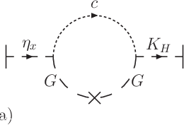
The Feynman graphs that give rise to the term ∂ηx(δ​I​Γ1−loop/δ​KH)\partial_{\eta_{x}}(\delta{\rm I}\hskip-1.9919pt\Gamma^{\mathrm{1-loop}}/\delta K_{H}) in (4.14) are shown in Fig. 1. Observe that for σ=1\sigma=1, only the graph in Fig. 1(a) contributes in this case.
Refer to caption
Refer to caption
Figure 1: The Feynman diagrams which contribute to the term ∂ηx(δ​I​Γ1−loop/δ​KH)\partial_{\eta_{x}}(\delta{\rm I}\hskip-1.9919pt\Gamma^{\mathrm{1-loop}}/\delta K_{H}) in (4.14). The second graph is required for σ≠1\sigma\neq 1 and takes account of the gauge dependence due to the Goldstone–gauge-boson mixing.

Let us first consider the RξR_{\xi} set of gauges, where σ=1\sigma=1. Calculating the Feynman graph in Fig. 1(a) at zero external momentum, we obtain

∂ηξ(δ​I​Γ1−loopδ​KH)=g2​v32​π2​[1λ​v2+m2​(mc2​ln⁡mc2μ¯2−mG2​ln⁡mG2μ¯2)+ 1+1ε].\partial_{\eta_{\xi}}\left(\frac{\delta{\rm I}\hskip-1.9919pt\Gamma^{\mathrm{1-loop}}}{\delta K_{H}}\right)\ =\ \frac{g^{2}v}{32\pi^{2}}\,\bigg[\,\frac{1}{\lambda v^{2}+m^{2}}\left(m_{c}^{2}\,\ln\frac{m_{c}^{2}}{\bar{\mu}^{2}}\>-\>m_{G}^{2}\,\ln\frac{m_{G}^{2}}{\bar{\mu}^{2}}\right)\ +\>1\>+\ \frac{1}{\varepsilon}\,\bigg]\;. (4.16)

Consequently, the gauge dependence of the 1-loop effective potential is determined by means of the NI (4.14):

∂ξ(Veff1−loop)Rξ\displaystyle\partial_{\xi}\Big(V^{\mathrm{1-loop}}_{\rm eff}\Big)_{R_{\xi}}\! =\displaystyle= g2​v232​π2[ξg2v2(lnλ​v2+m2+ξ​g2​v2μ¯2−lnξ​g2​v2μ¯2)\displaystyle\!\frac{g^{2}v^{2}}{32\pi^{2}}\,\bigg[\,\xi g^{2}v^{2}\bigg(\ln\frac{\lambda v^{2}+m^{2}+\xi g^{2}v^{2}}{\bar{\mu}^{2}}\ -\ \ln\frac{\xi g^{2}v^{2}}{\bar{\mu}^{2}}\,\bigg) (4.17)
+(λv2+m2)(lnλ​v2+m2+ξ​g2​v2μ¯2− 1−1ε)].\displaystyle\!+\ (\lambda v^{2}+m^{2})\,\bigg(\ln\frac{\lambda v^{2}+m^{2}+\xi g^{2}v^{2}}{\bar{\mu}^{2}}\ -\>1\>-\ \frac{1}{\varepsilon}\,\bigg)\,\bigg]\;.

It is easy to check that the above result coincides with that obtained after differentiating the analytical expression for the effective potential in  (3.5) with respect to ξ\xi.

We now turn to the non-trivial case of σ≠1\sigma\neq 1. In this case, one should consider the mixing between the would-be Goldstone boson GG and the gauge boson AμA^{\mu}, as shown in Fig. 1(b). In particular, taking both graphs of Fig. 1 into account, we may calculate the gauge dependence of the effective potential on the two GF parameters ξ\xi and σ\sigma:

∂ξ(Veff1−loop)Rξ/σ\displaystyle\partial_{\xi}\Big(V^{\mathrm{1-loop}}_{\rm eff}\Big)_{R_{\xi/\sigma}}\! =\displaystyle= g2​v232​π2{ξg2v2(lnλ​v2+m2+σ​ξ​g2​v2σ​μ¯2−lnξ​g2​v2μ¯2)\displaystyle\!\frac{g^{2}v^{2}}{32\pi^{2}}\bigg\{\;\xi g^{2}v^{2}\;\bigg(\ln\frac{\lambda v^{2}+m^{2}+\sigma\xi g^{2}v^{2}}{\sigma\bar{\mu}^{2}}\ -\ \ln\frac{\xi g^{2}v^{2}}{\bar{\mu}^{2}}\,\bigg) (4.18)
+12​(λ​v2+m2)1/2​[λ​v2+m2+4​ξσ​g2​v2​(σ−1)]1/2​ln⁡m¯G2m¯c2\displaystyle\!\hskip-17.07164pt+\ \frac{1}{2}\;(\lambda v^{2}+m^{2})^{1/2}\;\bigg[\;\lambda v^{2}\>+\>m^{2}\>+\>\frac{4\xi}{\sigma}\;g^{2}v^{2}(\sigma-1)\bigg]^{1/2}\;\ln\frac{\bar{m}_{G}^{2}}{\bar{m}_{c}^{2}}
+(λ​v2+m2)​(ln⁡m¯G2μ¯2+ln⁡m¯c2μ¯2+12​ln⁡mG2μ¯2+12​ln⁡mc2μ¯2− 2+1σ)\displaystyle\!\hskip-17.07164pt+\ (\lambda v^{2}+m^{2})\;\bigg(\,\ln\frac{\bar{m}_{G}^{2}}{\bar{\mu}^{2}}\ +\ \ln\frac{\bar{m}_{c}^{2}}{\bar{\mu}^{2}}\ +\ \frac{1}{2}\ln\frac{{m}_{G}^{2}}{\bar{\mu}^{2}}\ +\ \frac{1}{2}\ln\frac{{m}_{c}^{2}}{\bar{\mu}^{2}}\>-\ 2\ +\ \frac{1}{\sigma}\,\bigg)
−1ε(λv2+m2)(2−1σ)},\displaystyle\!\hskip-17.07164pt-\ \frac{1}{\varepsilon}\;(\lambda v^{2}+m^{2})\bigg(2-\frac{1}{\sigma}\bigg)\;\bigg\}\;,
∂σ−1(Veff1−loop)Rξ/σ\displaystyle\partial_{\sigma^{-1}}\Big(V^{\mathrm{1-loop}}_{\rm eff}\Big)_{R_{\xi/\sigma}}\! =\displaystyle= ξ​g2​v232​π2(λv2+m2)[1m¯G2−m¯c2(m¯G2lnm¯G2μ¯2−m¯c2lnm¯c2μ¯2)\displaystyle\!\frac{\xi g^{2}v^{2}}{32\pi^{2}}\ (\lambda v^{2}+m^{2})\;\bigg[\,\frac{1}{\bar{m}_{G}^{2}-\bar{m}_{c}^{2}}\ \bigg(\,\bar{m}_{G}^{2}\;\ln\frac{\bar{m}_{G}^{2}}{\bar{\mu}^{2}}\ -\ \bar{m}_{c}^{2}\;\ln\frac{\bar{m}_{c}^{2}}{\bar{\mu}^{2}}\,\bigg) (4.19)
− 1−1ε].\displaystyle\!\hskip-17.07164pt-\ 1\>-\ \frac{1}{\varepsilon}\;\bigg]\;.

Again, we have checked that the same result is obtained, if the analytical expression for the 1-loop effective potential in (3.6) is differentiated with respect to the GF parameters ξ\xi and σ−1\sigma^{-1}, in agreement with the NI.

From (4.18) and (4.19), it is then not difficult to prove the gauge independence of the 1-loop effective potential at its extrema. To zeroth order of loop expansion, the extrema of the Higgs potential, determined from (2.8), are

v= 0,v2=−m2λ.v\ =\ 0\;,\qquad v^{2}\ =\ -\frac{m^{2}}{\lambda}\ . (4.20)

Up to an unspecified additive cosmological constant, the first solution corresponding to a local maximum gives a vanishing effective potential, i.e. Veff1−loop​(v=0)=0V^{\mathrm{1-loop}}_{\mathrm{eff}}(v=0)=0, whereas the second one, v2=−m2/λv^{2}\ =\ -m^{2}/\lambda which corresponds to the global minimum of the effective potential to 𝒪⁡(ℏ){\cal O}(\hbar), gives

(Veff1−loop)Rξ/σ\displaystyle\Big(V^{\mathrm{1-loop}}_{\mathrm{eff}}\Big)_{R_{\xi/\sigma}}\! =\displaystyle= m464​π2[ 4ln−2​m2μ¯2− 2lnm2μ¯2− 3+g4λ2( 3lng2(−m2/λ)μ¯2−52)\displaystyle\!\frac{m^{4}}{64\pi^{2}}\ \bigg[\,4\ln\frac{-2m^{2}}{\bar{\mu}^{2}}\ -\ 2\ln\frac{m^{2}}{\bar{\mu}^{2}}\ -\ 3\ +\ \frac{g^{4}}{\lambda^{2}}\;\bigg(\,3\ln\frac{g^{2}(-m^{2}/\lambda)}{\bar{\mu}^{2}}\ -\ \frac{5}{2}\,\bigg) (4.21)
− 4∑i=1,2hi4λ2(lnhi2(−m2/λ)μ¯2−1)−1ε( 2+3​g2λ2−4∑i=1,2hi4λ2)].\displaystyle\!\hskip-42.67912pt-\ 4\;\sum_{i=1,2}\;\frac{h_{i}^{4}}{\lambda^{2}}\ \bigg(\,\ln\frac{h_{i}^{2}(-m^{2}/\lambda)}{\bar{\mu}^{2}}-1\bigg)\ -\ \frac{1}{\varepsilon}\bigg(\,2\>+\ \frac{3g^{2}}{\lambda^{2}}\ -4\,\frac{\sum_{i=1,2}\;h_{i}^{4}}{\lambda^{2}}\,\bigg)\;\bigg]\;.\qquad

This completes our proof that, up to 1-loop level, the vacuum energy of the Abelian Higgs model is gauge invariant in this general Rξ/σR_{\xi/\sigma} class of non-linear gauges.

5 1-loop Renormalization

In this section, we present the 1-loop constant and wavefunction renormalizations in the non-linear Rξ/σR_{\xi/\sigma} gauges in the MS¯\overline{\rm MS} scheme. To this end, we use the so-called displacement operator formalism, or DD-formalism in short, which was developed in [10] as an alternative approach to systematically performing renormalization to all orders in perturbation theory.

According to the DD-formalism, the renormalized 1PI nn-point correlation functions, denoted hereafter with a script RR, are related to the unrenormalized ones through:

ϕRn​I​ΓϕnR​(λR,σR,ξR,μ)=eD​(ϕRn​I​Γϕn​(λR,σR,ξR,μ,ε)),\phi_{R}^{n}\,{\rm I}\hskip-1.9919pt\Gamma^{R}_{\phi^{n}}(\lambda_{R},\sigma_{R},\xi_{R};\mu)\ =\ e^{D}\,\Big(\phi_{R}^{n}{\rm I}\hskip-1.9919pt\Gamma_{\phi^{n}}(\lambda_{R},\sigma_{R},\xi_{R};\mu,\varepsilon)\Big)\;, (5.1)

where DD is the displacement operator that takes on the form,

D=δ​ϕ​∂∂ϕR+δ​λ​∂∂λR+δ​σ​∂∂σR+δ​ξ​∂∂ξR,D\ =\ \delta\phi\frac{\partial}{\partial\phi_{R}}\>+\>\delta\lambda\frac{\partial}{\partial\lambda_{R}}\>+\>\delta\sigma\frac{\partial}{\partial\sigma_{R}}\>+\>\delta\xi\frac{\partial}{\partial\xi_{R}}\;, (5.2)

where ϕ\phi represents all the fields in the model and λ\lambda all the coupling and mass parameters, i.e. λ,m2,g,h1,2\lambda,\ m^{2},\ g,\ h_{1,2}, including the VEV vv of the Higgs field. In addition, the counterterm renormalizations, δ​ϕ\delta\phi, δ​λ\delta\lambda etc, are defined as, δ​ϕ=ϕ−ϕR=(Zϕ1/2−1)​ϕR\delta\phi=\phi-\phi_{R}=(Z^{1/2}_{\phi}-1)\phi_{R}, δ​λ=λ−λR=(Zλ−1)​λR\delta\lambda=\lambda-\lambda_{R}=(Z_{\lambda}-1)\lambda_{R} etc. Since the Rξ/σR_{\xi/\sigma} gauge obeys the HLET, vv does not need to have its own counterterm and it is renormalized via the Higgs wavefunction, i.e. v=ZH12​vRv=Z_{H}^{\frac{1}{2}}v_{R}.

We may now perform a loopwise expansion of the operator eDe^{D} in (5.1),

eD=1+D(1)+(D(2)+12​D(1)​2)+…e^{D}=1+D^{(1)}+(D^{(2)}+\frac{1}{2}D^{(1)2})+... (5.3)

where the superscript (n)(n) on DD denotes the loop order, i.e.

D(n)=δ​ϕ(n)​∂∂ϕR+δ​λ(n)​∂∂λR+δ​σ(n)​∂∂σR+δ​ξ(n)​∂∂ξR.D^{(n)}\ =\ \delta\phi^{(n)}\frac{\partial}{\partial\phi_{R}}\>+\>\delta\lambda^{(n)}\frac{\partial}{\partial\lambda_{R}}\>+\>\delta\sigma^{(n)}\frac{\partial}{\partial\sigma_{R}}\>+\>\delta\xi^{(n)}\frac{\partial}{\partial\xi_{R}}\;. (5.4)

Correspondingly, the parameter or counterterm shifts δ​ϕ(n),δ​λ(n),δ​σ(n)\delta\phi^{(n)},\ \delta\lambda^{(n)},\ \delta\sigma^{(n)} and δ​ξ(n)\delta\xi^{(n)} are loopwise defined as

δ​ϕ(n)=Zϕ12​(n)​ϕR,δ​λ(n)=Zλ(n)​λR,δ​σ(n)=Zσ(n)​σR,δ​ξ(n)=Zξ(n)​ξR.\delta\phi^{(n)}\ =\ Z_{\phi}^{\frac{1}{2}(n)}\phi_{R},\qquad\delta\lambda^{(n)}\ =\ Z_{\lambda}^{(n)}\lambda_{R},\qquad\delta\sigma^{(n)}\ =\ Z_{\sigma}^{(n)}\sigma_{R},\qquad\delta\xi^{(n)}\ =\ Z_{\xi}^{(n)}\xi_{R}\ . (5.5)

Applying the DD-formalism to 1-loop, we have

ϕRn​ΓϕnR⁡(1)​(λR,σR,ξR,μ)=D(1)​(ϕRn​Γϕn(0)​(λR,σR,ξR,μ))+ϕRn​Γϕn(1)​(λR,σR,ξR,μ,ε).\phi_{R}^{n}\Gamma^{R(1)}_{\phi^{n}}(\lambda_{R},\sigma_{R},\xi_{R};\mu)\ =\ D^{(1)}\left(\phi_{R}^{n}\Gamma^{(0)}_{\phi^{n}}(\lambda_{R},\sigma_{R},\xi_{R};\mu)\right)+\phi_{R}^{n}\Gamma^{(1)}_{\phi^{n}}(\lambda_{R},\sigma_{R},\xi_{R};\mu,\varepsilon)\;. (5.6)

Employing (5.6) in the MS¯\overline{\rm MS} scheme, we may calculate the 1-loop constant and wavefunction renormalizations in the non-linear Rξ/σR_{\xi/\sigma} gauge. These are given by

ZH\displaystyle Z_{H} =\displaystyle= 1+1(4​π)2​ε​(3​g2+ξ​g2−2​∑i=12hi2+ξ​g2σ​(σ−1)),\displaystyle 1+\frac{1}{(4\pi)^{2}\varepsilon}\left(3g^{2}+\xi g^{2}-2\sum_{i=1}^{2}h_{i}^{2}+\frac{\xi g^{2}}{\sigma}(\sigma-1)\right)\;,
ZG\displaystyle Z_{G} =\displaystyle= 1+1(4​π)2​ε​(3​g2−3​ξ​g2−2​∑i=12hi2+ξ​g2σ​(σ−1)),\displaystyle 1+\frac{1}{(4\pi)^{2}\varepsilon}\left(3g^{2}-3\xi g^{2}-2\sum_{i=1}^{2}h_{i}^{2}+\frac{\xi g^{2}}{\sigma}(\sigma-1)\right)\;,
Zσ\displaystyle Z_{\sigma} =\displaystyle= 1+1(4​π)2​ε​(−3​g2+3​ξ​g2+2​λ+2​∑i=12hi2−ξ​g2σ​(σ−1)+ξ​g2σ​(σ−1)2),\displaystyle 1+\frac{1}{(4\pi)^{2}\varepsilon}\left(-3g^{2}+3\xi g^{2}+2\lambda+2\sum_{i=1}^{2}h_{i}^{2}-\frac{\xi g^{2}}{\sigma}(\sigma-1)+\frac{\xi g^{2}}{\sigma}(\sigma-1)^{2}\right)\;,
Zξ\displaystyle Z_{\xi} =\displaystyle= 1+1(4​π)2​ε​(−143​g2+2​ξ​g2+2​λ+2​∑i=12hi2−2​ξ​g2σ​(σ−1)),\displaystyle 1+\frac{1}{(4\pi)^{2}\varepsilon}\left(-\frac{14}{3}g^{2}+2\xi g^{2}+2\lambda+2\sum_{i=1}^{2}h_{i}^{2}-2\frac{\xi g^{2}}{\sigma}(\sigma-1)\right)\;,
ZA\displaystyle Z_{A} =\displaystyle= 1+1(4​π)2​ε​(−53​g2),\displaystyle 1+\frac{1}{(4\pi)^{2}\varepsilon}\left(-\frac{5}{3}g^{2}\right)\;,
Zc\displaystyle Z_{c} =\displaystyle= 1,\displaystyle 1\;,
Zg\displaystyle Z_{g} =\displaystyle= 1+1(4​π)2​ε​(56​g2),\displaystyle 1+\frac{1}{(4\pi)^{2}\varepsilon}\left(\frac{5}{6}g^{2}\right)\;,
Zλ\displaystyle Z_{\lambda} =\displaystyle= 1+1(4​π)2​ε​(−6​g2+10​λ+4​∑i=12hi2+3​g2λ−4​∑i=12hi4λ),\displaystyle 1+\frac{1}{(4\pi)^{2}\varepsilon}\left(-6g^{2}+10\lambda+4\sum_{i=1}^{2}h_{i}^{2}+\frac{3g^{2}}{\lambda}-\frac{4\sum_{i=1}^{2}h_{i}^{4}}{\lambda}\right)\;,
Zm2\displaystyle Z_{m^{2}} =\displaystyle= 1+1(4​π)2​ε​(−3​g2+4​λ+2​∑i=12hi2),\displaystyle 1+\frac{1}{(4\pi)^{2}\varepsilon}\left(-3g^{2}+4\lambda+2\sum_{i=1}^{2}h_{i}^{2}\right)\;,
Z1,2L\displaystyle Z_{1,2}^{L} =\displaystyle= 1+1(4​π)2​ε​(−g2​ξ−h1,22+ξ​g2σ​(σ−1)),\displaystyle 1+\frac{1}{(4\pi)^{2}\varepsilon}\left(-g^{2}\xi-h_{1,2}^{2}+\frac{\xi g^{2}}{\sigma}(\sigma-1)\right)\;,
Z1,2R\displaystyle Z_{1,2}^{R} =\displaystyle= 1+1(4​π)2​ε​(−h1,22),\displaystyle 1+\frac{1}{(4\pi)^{2}\varepsilon}\left(-h_{1,2}^{2}\right)\;,
Zh1,2\displaystyle Z_{h_{1,2}} =\displaystyle= 1+1(4​π)2​ε​(−32​g2+h1,22+∑i=12hi2+2​ξ​g2σ​(σ−1)).\displaystyle 1+\frac{1}{(4\pi)^{2}\varepsilon}\left(-\frac{3}{2}g^{2}+h_{1,2}^{2}+\sum_{i=1}^{2}h_{i}^{2}+2\frac{\xi g^{2}}{\sigma}(\sigma-1)\right)\;. (5.7)

Observe that Green’s functions in the RξR_{\xi} gauge, where σR=1\sigma_{R}=1, would require an additional renormalization constant, given by δ​σ(1)=Zσ=1(1)−1\delta\sigma^{(1)}=Z_{\sigma=1}^{(1)}-1, beyond the 1-loop level, in order to render them ultra-violet finite. For instance, this will be the case, when one is computing nn-point correlation functions that involve Higgs bosons or left-handed fermions in the Abelian Higgs model under study. The only exception to this is the Landau gauge ξ=0+\xi=0^{+}, which does not require a renormalization counterterm. The reason is that unlike σ\sigma, the GF parameter ξ\xi renormalizes multiplicatively, so the condition ξ=0\xi=0 will not be affected by renormalization. Moreover, in the Landau gauge, the role of the GF parameter σ\sigma is redundant, since any σ\sigma-dependence of the counterterms contains a factor of ξ\xi as well and therefore it vanishes in the limit ξ→0+\xi\to 0^{+} [cf. (5.7)].

6 Conclusions

We have calculated the 1-loop effective potential of an Abelian Higgs model within the Rξ/σR_{\xi/\sigma} class of non-linear gauges. The Rξ/σR_{\xi/\sigma} class involves two GF parameters ξ\xi and σ\sigma and constitutes a renormalizable extension of the Feynman–’t Hooft RξR_{\xi} set of gauges. In particular, it enables one to consistently study the gauge dependence of nn-point correlation functions beyond the 1-loop level. Another advantage of the Rξ/σR_{\xi/\sigma} GF scheme is that it preserves the Higgs-boson low-energy theorem, which has found to have several applications in particle phenomenology [8] including those in BB-meson physics [18].

In the Rξ/σR_{\xi/\sigma} class of gauges, one has to properly consider Goldstone–gauge-boson mixing effects. Taking these effects into account, we have shown that the 1-loop effective potential evaluated at its extrema is independent of both the GF parameters ξ\xi and σ\sigma. This result is in agreement with the Nielsen identity, which we have derived here for the Abelian Higgs model in the Rξ/σR_{\xi/\sigma} gauge.

It is important to stress that the Goldstone–gauge-boson mixing vanishes at the tree level in the Feynman–’t Hooft RξR_{\xi} set of gauges, when σ=1\sigma=1, and in the Landau gauge ξ=0+\xi=0^{+}. Unlike in the Landau gauge, however, the mixing of the gauge field with its associated would-be Goldstone boson will reappear beyond the 1-loop level within the frequently used Feynman σ=1\sigma=1 gauge. We have therefore calculated the 1-loop counterterms for couplings, masses and field wavefunctions within the general Rξ/σR_{\xi/\sigma} class of gauges, for arbitrary values of the σ\sigma parameter. We hope that the pivotal study presented in this paper will be useful for future higher-order calculations and cross-checks of gauge independence of physical observables, within more realistic models of particle physics.

Acknowledgements

This work is supported in part by the STFC research grant: PP/D000157/1.

References

  • [1] S. R. Coleman and E. Weinberg, Phys. Rev. D 7 (1973) 1888.
  • [2] J. Goldstone, A. Salam and S. Weinberg, Phys. Rev. 127 (1962) 965.
  • [3] G. Jona-Lasinio, Nuovo Cim. 34 (1964) 1790.
  • [4] For instance, see,
    B. A. Bassett, S. Tsujikawa and D. Wands, Rev. Mod. Phys. 78 (2006) 537.
  • [5] J. I. Kapusta, Finite-Temperature Field Theory, Cambridge University Press, Cambridge, UK, 1989.
  • [6] N. K. Nielsen, Nucl. Phys. B 97 (1975) 527; Nucl. Phys. B 101 (1975) 173.
  • [7] A. Pilaftsis, Phys. Lett. B 422 (1998) 201.
  • [8] J. R. Ellis, M. K. Gaillard and D. V. Nanopoulos, Nucl. Phys. B 106 (1976) 292;
    M. A. Shifman, A. I. Vainshtein and V. I. Zakharov, Phys. Lett. B 78 (1978) 443;
    M. A. Shifman, A. I. Vainshtein, M. B. Voloshin and V. I. Zakharov, Sov. J. Nucl. Phys. 30 (1979) 711 [Yad. Fiz. 30 (1979) 1368].
  • [9] For reviews, see,
    M. A. Shifman, Phys. Rept. 209 (1991) 341;
    S. Dawson and H. E. Haber, Int. J. Mod. Phys. A 7 (1992) 107.
  • [10] D. Binosi, J. Papavassiliou and A. Pilaftsis, Phys. Rev. D 71 (2005) 085007.
  • [11] B. M. Kastening, Phys. Rev. D 51 (1995) 265.
  • [12] I. J. R. Aitchison and C. M. Fraser, Annals Phys. 156 (1984) 1;
    D. Metaxas and E. J. Weinberg, Phys. Rev. D 53 (1996) 836;
    D. Metaxas, Phys. Rev. D 63 (2001) 085009.
  • [13] C. Becchi, A. Rouet and R. Stora, Ann. Phys. (N.Y.) 98 (1976) 287.
  • [14] R. Jackiw, Phys. Rev. D 9 (1974) 1686.
  • [15] J. Zinn-Justin, Quantum Field Theory and Critical Phenomena, Fourth Edition, Oxford University Press, Great Clarendon Street, Oxford, UK, 2002.
  • [16] O. Piguet and K. Sibold, Nucl. Phys. B 253 (1985) 517.
  • [17] R. Häussling and E. Kraus, Z. Phys. C 75 (1997) 739.
  • [18] J. Ellis, J. S. Lee and A. Pilaftsis, Phys. Rev. D 76 (2007) 115011;
    R. N. Hodgkinson and A. Pilaftsis, arXiv:0807.4167 [hep-ph].