Perturbative approach to an exactly solved problem : the Kitaev honeycomb model

The model considered in this work is a spin-$1/2$ system proposed by Kitaev [7] in which spins are located at the vertices of a honeycomb lattice. Since the honeycomb lattice is topologically equivalent to the brick-wall lattice, we shall always represent it as shown in Fig. 1a. In this lattice, one distinguishes three types of links ($x$, $y$, and $z$) to which one associates three different couplings and interactions. The Hamiltonian of the system is

where $\sigma_{i}^{\alpha}$ are the usual Pauli matrices at site $i$. In the following we assume, without loss of generality[7], that $J_{\alpha}\geq 0$ for all $\alpha$ and $J_{z}\geq J_{x},J_{y}$.

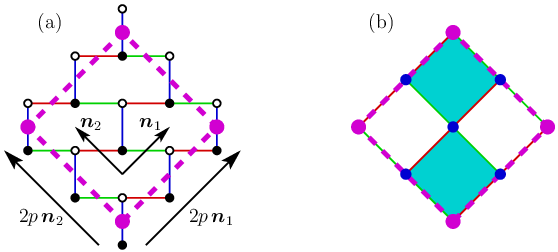
We will either work with an infinite system and open boundary conditions (a plane), or with a finite (or infinite) system and periodic boundary conditions (a torus). In the latter case and for reasons that will become clearer in the following (in particular, see Sec. V.2), we shall restrict ourselves to the periodic boundary conditions (PBC) depicted in Fig. 2. The number of sites $N_{\mathrm{s}}$ is $N_{\mathrm{s}}=2(2p)^{2}=8p^{2}$, with $p\in\mathbb{N}$ ($p=1$ in Fig. 2a). Let us anticipate what follows and mention that these boundary conditions are such that the lattice of $z$-dimers (Fig. 1b) can be bi-colored as shown in Fig. 2b).

A remarkable property of Hamiltonian (1), is that its elementary operators $K_{ij}=\sigma_{i}^{\alpha}\sigma_{j}^{\alpha}$ commute with plaquette operators $W_{p}$ so that $\left[H,W_{p}\right]=0$. For the plaquette $p$ shown in Fig. 1a, such an operator is defined as

Let us mention that in the expression of $W_{p}$ in terms of the $K$’s, one could have started at any site instead of site $1$ and/or one could have taken the product of $K^{\prime}s$ anti-clockwise instead of clockwise. Furthermore, the expression in terms of $\sigma$’s could also be written $W_{p}=\prod_{i}\sigma_{i}^{\mathrm{out}(i)}$ where $i$ runs over the set of six spins around the plaquette $p$, and where the notation $\mathrm{out}(i)$ means the “outgoing” direction at site $i$, with respect to the plaquette’s contour. An illustration of the $W_{p}$ operator is given in Fig. 3.

Since $W_{p}^{2}=\mathbb{I}$, the eigenvalues of the plaquette operators are $w_{p}=\pm 1$. Note that $\left[W_{p},W_{p^{\prime}}\right]=0$, as can be shown from the usual Pauli matrices algebra. As a consequence, $H$ and the $W_{p}$’s can be diagonalized simultaneously. Following Kitaev, we will call a vortex sector a subspace of the Hilbert space with a given map of the $w_{p}$’s. By definition a vortex is a plaquette for which $w_{p}=-1$, so that for example, the vortex-free sector is defined by $w_{p}=+1$ for all $p$’s.

In fact, all loop operators made of “outgoing spins” (see Figs. 4 and 5) are conserved and all commute with each other, which can be verified in the same way as for the $W_{p}$’s. However, not all of them can be set independently to $\pm 1$. Some relations among them arise from the following fact (which can be checked by studying all possible cases) : the product of $W_{p}$ and a nearby loop operator $\mathcal{L}$ gives a new loop operator $\mathcal{L}^{\prime}=W_{p}\mathcal{L}$, as illustrated on a particular example in Fig. 4.

As an illustration of other relations involving loop operators around the torus, with the loops of Fig. 5 one has

where we have denoted, for example, $\mathcal{L}_{\mathrm{a}}=\prod_{i\in\mathcal{C}_{\mathrm{a}}}\sigma_{i}^{\mathrm{out}(i)}$. The minus sign in the last equation above comes from the crossing of $\mathcal{L}_{\mathrm{b}}$ and $\mathcal{L}_{\mathrm{c}}$. In the three expressions above, the product of plaquette operators could also have been taken over the complementary set of plaquettes. Indeed, on the torus the relations among loop operators yield the following constraint

showing in particular that the number of vortices has to be even in a system with PBC.

From examples shown in Fig. 5, one can deduce that all $W_{p}$’s [except one, because of Eq. (6)], $\mathcal{L}_{\mathrm{b}}$ and $\mathcal{L}_{\mathrm{c}}$ can be set independently to $\pm 1$, which then imposes all other conserved quantities.

The above discussed local conserved quantities are not sufficient to fully diagonalize the Hamiltonian. Indeed, if $N_{\mathrm{s}}$ is the number of sites, then there is a total of $N=N_{\mathrm{s}}/2$ plaquettes, but only $N-1$ independent ones. With the two cycles around the torus, this gives $N+1$ independent conserved quantities, which is obviously smaller than $N_{\mathrm{s}}$.

However, $H$ has a crucial property : it can be transformed into a free Majorana fermions Hamiltonian and is thus exactly solvable. Let us also mention that another solution based on the Jordan-Wigner transformation maps the spin Hamiltonian $H$ onto a spinless fermions system with $p$-wave pairing [9, 11, 12].

As shown by Kitaev [7], the ground state of $H$ lies in the vortex-free sector and the phase diagram contains, in this sector, two phases : a gapped phase for $J_{z}>J_{x}+J_{y}$ and a gapless phase for $J_{z}\leq J_{x}+J_{y}$. In the gapped phase the low-energy excitations are Abelian anyons (semions) whereas in the gapless phase, the low-energy excitations are fermionic. The gapless phase acquires a gap in the presence of a magnetic field and then contains gapped non-Abelian anyon excitations. The phase diagram has also been investigated in other vortex configurations such as the vortex-full sector and similar phases have been obtained. More precisely, one has a gapped phase for $J_{z}^{2}>J_{x}^{2}+J_{y}^{2}$ and a gapless phase in the opposite case[14].

Our goal here is to determine the low-energy spectrum for any vortex configuration. Of course, one may use the fermionic Hamiltonian mentioned above but, it can only be exactly diagonalized for translation-invariant configuration. Here, we follow an alternative route by focusing on the isolated-dimer limit $J_{z}\gg J_{x},J_{y}$.

The very first step of our analysis consists in mapping the four possible states of the two spins of a $z$-dimer onto those of an effective spin and a hardcore boson. More precisely, denoting $|\!\uparrow\rangle$ ($|\!\downarrow\rangle$) the eigenstate of $\sigma_{z}$ with eigenvalue $+1$ ($-1$), an isolated $z$-dimer can be in one of the two low-energy states $\{|\!\uparrow\uparrow\rangle,|\!\downarrow\downarrow\rangle\}$ with energy $-J_{z}$, or in one of the two high-energy states $\{|\!\uparrow\downarrow\rangle,|\!\downarrow\uparrow\rangle\}$ with energy $+J_{z}$. Keeping in mind that our aim is to perform a perturbation theory in the limit $J_{z}\gg J_{x},J_{y}$, it is natural to interpret the change from a ferromagnetic to an anti-ferromagnetic configuration as the creation of a particle with an energy cost $2\,J_{z}$. By construction, such a particle is a hardcore boson. The remaining degree of freedom can be described by a spin 1/2, indicating which of the two configurations is realized. There are many possible parametrizations but here we choose the following

The left (right) spin is the one of the black (white) site of the dimer ($|\!\uparrow\downarrow\rangle=|\!\uparrow_{\bullet}\downarrow_{\circ}\rangle$, etc). Double arrows represent the state of the effective spin which is here the same as the state of the left (black) spin.

Within such a mapping, effective spins and hardcore bosons live on the effective square lattice of $z$-dimers (see Fig. 1). This lattice is shown again in Fig. 2b, together with the PBC, which are such that it can be bi-colored. In what follows, the sites of the effective lattice will be denoted with bold letters, such as ${\boldsymbol{i}}$.

Let us now write the Hamiltonian (1) in this language. Therefore, we first translate the action of the spin operators in the effective-spin boson (ESB) formalism. It is easy to check that one has

The operators $\tau^{\alpha}_{\boldsymbol{i}}$ ($\alpha=x,y,z$) are the Pauli matrices acting on the effective spin at site ${\boldsymbol{i}}$, while $b^{\phantom{\dagger}}_{\boldsymbol{i}}$ and $b^{\dagger}_{\boldsymbol{i}}$ are hardcore bosonic annihilation and creation operators, satisfying the usual on-site anticommutation relation $\{b^{\phantom{\dagger}}_{\boldsymbol{i}},b^{\dagger}_{\boldsymbol{i}}\}=\mathbb{I}$ (and operators on different sites commute). Setting once for all $J_{z}=1/2$ so that creating a boson costs an energy $1$ in the isolated-dimer limit, the Hamiltonian (1) reads

where $N$ is the number of $z$-dimers (or, equivalently, of square plaquettes), and

These operators are built from local hopping and pair creation operators

We emphasize that the mapping (8) explicitly breaks the symmetry between white and black sites of the original brick-wall lattice. This is responsible for the apparent breaking of symmetry between the $x/{\boldsymbol{n}}_{1}$ and $y/{\boldsymbol{n}}_{2}$ directions in Eq. (13). However, for all the physically observable results, this symmetry remains intact (see for example the series expansion of eigenenergies in Appendix C). Note however that the ${\boldsymbol{n}}_{1}+{\boldsymbol{n}}_{2}$ and ${\boldsymbol{n}}_{1}-{\boldsymbol{n}}_{2}$ directions are not equivalent, as can be seen from the underlying brick-wall lattice.

Let us now rephrase the conserved operators discussed in Sec. II.2 in the effective language. Using the notations depicted in Fig. 1b, as well as the mapping (8), the plaquette operators transform into

Note that $(-1)^{b^{\dagger}_{\boldsymbol{i}}b^{\phantom{\dagger}}_{\boldsymbol{i}}}=1-2b^{\dagger}_{\boldsymbol{i}}b^{\phantom{\dagger}}_{\boldsymbol{i}}$. In the same vein, for the cycles around the torus shown in Figs. 5b-5c, which are reproduced for the effective lattice in Figs. 6b-6c, one has $\mathcal{L}_{\mathrm{b}}=\prod_{{\boldsymbol{i}}\in\mathcal{C}_{\mathrm{b}}}\left[-(-1)^{b^{\dagger}_{\boldsymbol{i}}b^{\phantom{\dagger}}_{\boldsymbol{i}}}\tau^{x}_{\boldsymbol{i}}\right]=\prod_{{\boldsymbol{i}}\in\mathcal{C}_{\mathrm{b}}}\left[(-1)^{b^{\dagger}_{\boldsymbol{i}}b^{\phantom{\dagger}}_{\boldsymbol{i}}}\tau^{x}_{\boldsymbol{i}}\right]$ (since there is an even number of sites on the contour with the PBC chosen here), as well as $\mathcal{L}_{\mathrm{c}}=\prod_{{\boldsymbol{i}}\in\mathcal{C}_{\mathrm{c}}}\tau^{x}_{\boldsymbol{i}}$. The expression for $\mathcal{L}_{\mathrm{d}}$ (see Fig. 5d), namely $\mathcal{L}_{\mathrm{d}}=\prod_{{\boldsymbol{i}}\in\mathcal{C}_{\mathrm{d}}}\omega_{\boldsymbol{i}}$, is a bit more complicated, but it should be clear from Fig. 6d what the $\omega_{\boldsymbol{i}}$’s are. Finally, for the contour shown in Fig. 6a (which is in correspondence with Fig. 5a), one has $\prod_{p\subset\mathcal{C}_{\mathrm{a}}}W_{p}=\prod_{{\boldsymbol{i}}\in\mathcal{C}_{\mathrm{a}}}\omega_{\boldsymbol{i}}=\mathcal{L}_{\mathrm{a}}$ with the $\omega_{\boldsymbol{i}}$’s indicated in the figure, and with $p\subset\mathcal{C}_{\mathrm{a}}$ meaning the plaquettes $p$ enclosed in the contour $\mathcal{C}_{\mathrm{a}}$. With these notations, one can easily check that Eq. (5) still holds.

The elementary hopping and pair creation operators, namely $t_{\boldsymbol{i}}^{\boldsymbol{j}}$ and $v_{\boldsymbol{i}}^{\boldsymbol{j}}$ with ${\boldsymbol{i}}$ and ${\boldsymbol{j}}$ nearest neighbors, have a very remarkable property : they all commute with the $W_{p}$’s, as well as with any other loop operator

The original spin problem on the honeycomb lattice is thus mapped onto a quadratic hardcore boson problem on an effective square lattice, with conserved plaquette and loop operators. Let us underline that this mapping is exact and just provides an alternative description of the spin problem. The resulting Hamiltonian (9) remains difficult to diagonalize (except, of course, if one remembers that the model can be fermionized), since (i) bosons are hard core which prevents the use of a Bogoliubov transformation, (ii) bosonic and spin degrees of freedom are correlated. The conserved plaquette operators will of course be useful in simplifying and solving the problem as recently underlined in Ref. 15.

The starting point of the present perturbation theory is the isolated-dimer limit, namely $J_{x}=J_{y}=0$. In this limit, the spectrum is made of equidistant and degenerate levels separated by an energy gap $\Delta=2J_{z}=1$. To compute the perturbative spectrum, there are of course several methods among which the Green’s function formalism initially used by Kitaev [7]. However, if this approach is efficient to obtain the first nontrivial (nonconstant) correction, it becomes tricky to implement at higher orders.

Here, following Ref. 13, we use an alternative approach based on continuous unitary transformations (CUTs) conjointly proposed by Wegner [34] and Głazek and Wilson [35, 36]. We refer the interested reader to Ref. 37 for a recent pedagogical introduction. Its perturbative version denoted PCUTs is especially well-suited to the problem at hand. This technique is detailed in several works [38, 39]. Let us simply mention that the CUTs method requires the choice of a generator that drives the flow of the operators. All the results given here have been obtained with the so-called quasiparticle number-conserving generator first proposed by Mielke [40] for finite matrices and generalized to many-body systems by Knetter and Uhrig[39].

The latter have computed the perturbative expansion for any Hamiltonian of the form

provided two hypothesis are satisfied:

• •

  the unperturbed Hamiltonian $Q$ has an equidistant spectrum bounded from below ;

• •

  the perturbing Hamiltonian $\sum_{n=-2}^{+2}T_{n}$ is such that $[Q,T_{n}]=n\,T_{n}$.

Clearly, the Hamiltonian (9) meets these two criteria (up to a constant term) noting that in the present case, one has $T_{\pm 1}=0$. Here, we have included the ”small” parameters, namely $J_{x}$ and $J_{y}$, in the definition of the $T_{n}$ operators, which is not the convention usually adopted in the CUTs community.

The CUTs method together with the quasiparticle number-conserving generator unitarily transforms the Hamiltonian (16) into an effective Hamiltonian $H_{\mathrm{eff}}=U^{\dagger}HU$ commuting with $Q$, $U$ being a unitary operator. We give the first terms of the expansion up to order 4 in Appendix A. As can be seen in Table 1, the number of terms appearing in the perturbative expansion quickly increases with the order. For instance, at order 2, the effective Hamiltonian reads in our case

whereas at order 10, there are more than $10^{4}$ operators to consider.

Writing $H_{\mathrm{eff}}$ this way is only the very first part of the job since one next has to (i) determine its action in each subspace of a given quasiparticle (QP) number $q$ ; (ii) diagonalize $H_{\mathrm{eff}}$ in each of these subspaces. This is the object of the next sections : we first study the lowest-energy states ($q=0$ QP) which is the main contribution of our work ; then we turn to the $q=1$ QP states and recover the high-energy gap from the QP dispersion ; we end by $q\geqslant 2$ QP states, whose properties determine the statistics of the QPs, and we will see that the QPs behave as fermions which are, furthermore, non interacting. This fact is at the origin of a tremendous simplification of the effective Hamiltonian. Indeed, we found that $H_{\mathrm{eff}}$ can be written, at all orders and in the thermodynamical limit, as

We shall discuss each term in detail in the following sections, but let us mention that $E_{0}$, $\mu$, the $C$’s and the $D$’s are coefficients whose series expansion are computed. The $S$ operators are strings of spin operators $\tau_{\boldsymbol{j}}^{\alpha}$ and of phase factors $(-1)^{b^{\dagger}_{\boldsymbol{j}}b^{\phantom{\dagger}}_{\boldsymbol{j}}}$ on the cluster $\{{\boldsymbol{j}}_{1},\ldots,{\boldsymbol{j}}_{n}\}$. This very special form of multi-particle terms [remember $(-1)^{b^{\dagger}_{\boldsymbol{j}}b^{\phantom{\dagger}}_{\boldsymbol{j}}}=1-2b^{\dagger}_{\boldsymbol{j}}b^{\phantom{\dagger}}_{\boldsymbol{j}}$], leading to phase factors and spin-strings only, is responsible for the emergence of fermions in the model.

For a finite-size system with PBC, new terms appear in the effective Hamiltonian. They involve loop operators around the torus, and appear at a minimal order being the linear size $2p$ of the lattice. Such loop operators are associated to contours as the ones shown in Figs. 5 and 6, namely $\mathcal{L}_{\mathrm{b}}$, $\mathcal{L}_{\mathrm{c}}$ and $\mathcal{L}_{\mathrm{b}}^{\prime}$ for the contours $\mathcal{C}_{\mathrm{b}}$, $\mathcal{C}_{\mathrm{c}}$ and $\mathcal{C}_{\mathrm{b}}^{\prime}$. The presence of such loop operators in the effective Hamiltonian shows that the eigenstates of the Hamiltonian are also eigenstates of these loop operators. Their effect is to lift the degeneracies between states (which for each energy is at least four in the thermodynamical limit, since some of the excitations are Abelian semions and the genus of a torus is 1, see Ref. 5). We shall not dive into the details of such finite-size corrections, since our approach allows us to directly tackle with the most interesting thermodynamical limit. However, let us make a remark about a numerical check of this statement for small system sizes. For a torus whose linear size is strictly smaller than 4, the loop operator terms around the torus dominate the expansion over the $W_{p}$’s, and for a size of 4 both types of terms start contributing at the same order. One should thus not be surprised to find a ground-state for $p=1$ which is not in the vortex-free sector [15].

Before we turn to a detailed analysis of each QP subspace, let us show that we do not miss any state using simple counting arguments. We have already seen in Sec. II, that one has $N+2$ conserved $\mathbb{Z}_{2}$ quantities (two loop operators, and $N$ plaquette operators), with the constraint $\prod_{p}W_{p}=\mathbb{I}$. There is in fact one more relation between the $W_{p}$’s, involving the number of bosons, which reads

showing that the parity of the number of vortices living on white plaquettes (see Fig. 2) has to be the same as the parity of the number of bosons. The last equality simply comes from the previously mentioned constraint (6). The first equality can be checked using the expression (14) of the $W_{p}$’s. Indeed, for a site ${\boldsymbol{i}}$ having a white plaquette on its left, and another one on its right, the product of the two associated $W_{p}$’s will give $\tau_{\boldsymbol{i}}^{y}\times(-1)^{b^{\dagger}_{\boldsymbol{i}}b^{\phantom{\dagger}}_{\boldsymbol{i}}}\tau_{\boldsymbol{i}}^{y}=(-1)^{b^{\dagger}_{\boldsymbol{i}}b^{\phantom{\dagger}}_{\boldsymbol{i}}}$. In the same way, for a site ${\boldsymbol{i}}$ having a white plaquette above it, and another one under it, the product of the two associated $W_{p}$’s will give $\tau_{\boldsymbol{i}}^{z}\times(-1)^{b^{\dagger}_{\boldsymbol{i}}b^{\phantom{\dagger}}_{\boldsymbol{i}}}\tau_{\boldsymbol{i}}^{z}=(-1)^{b^{\dagger}_{\boldsymbol{i}}b^{\phantom{\dagger}}_{\boldsymbol{i}}}$. Let us note that (19) has a meaning in the two bases we are working in, the initial one and the unitarily transformed one. Indeed, in the initial basis, the Hamiltonian $H$ commutes with the parity operator $(-1)^{Q}$ ; in the rotated basis, $H_{\mathrm{eff}}$ commutes with $Q$.

We thus see that in a subspace with a given number of QP’s, there are $N$ independent conserved $\mathbb{Z}_{2}$ quantities. Thus, $N$ being the number of effective spins $\tau_{\boldsymbol{i}}$, there is no remaining effective spin degree of freedom once the $\mathbb{Z}_{2}$ quantities are chosen. As a conclusion, the $q$-QP subspace has dimension $d_{q}=2^{N}\begin{pmatrix}N\\ q\end{pmatrix}$, with the usual notation for binomial coefficients. This shows that we miss no state, since

where $N_{\mathrm{s}}$ is the total number of spins in the brick-wall lattice.

This discussion furthermore sheds light on the fact that in order to compute eigenenergies, a perturbative expansion of the Kitaev model (as opposed to exact numerics) is really of interest only in the $0$-QP subspace. Indeed, we have just seen that there are $N$ independent $\mathbb{Z}_{2}$ conserved quantities. It is thus clear that as soon as we will have written down the effective Hamiltonian in the $0$-QP subspace, the Hamiltonian will already be diagonal, whatever the vortex configuration, although writing down the eigenstates of the $\mathbb{Z}_{2}$ quantities in the basis of effective spin operators still has to be done. However, in the $1$-QP subspace, one will have to diagonalize an $N\times N$ matrix (numerically in the case of a nonperiodic vortex configuration), which is identical to what one has to do when solving the problem exactly as Kitaev did. For $q\geqslant 2$, the perturbative expansion looks even more complicated than the exact solution, but this is an artifact, since we recover free fermions.

In the 0-QP sector, and in the thermodynamical limit the effective Hamiltonian (18) simplifies and reads

where $\{p_{1},p_{2},\ldots,p_{n}\}$ denotes a set of $n$ plaquettes and the $W_{p}$’s are the conserved plaquette operators introduced in Sec. II. Note than when restricted to the 0-QP sector they simplify to $\left.W_{p}\right|_{q=0}=\tau_{\mbox{\tiny L}}^{y}\,\tau_{\mbox{\tiny U}}^{z}\,\tau_{\mbox{\tiny R}}^{y}\,\tau_{\mbox{\tiny D}}^{z}$ [see Eq. (14)].

As mentioned at the end of the previous section, obtaining eigenenergies only requires a minimal amount of work, namely replacing each $W_{p}$ by numbers $w_{p}=\pm 1$, and doing the same with loop operators, without forgetting about the constraints among these quantities. The perturbative expansion of the coefficients $E_{0}$ and $C_{p_{1},\ldots,p_{n}}$ are given in Appendix C. Let us note that $\{p_{1},p_{2},\ldots,p_{n}\}$ does not need to be a linked cluster of plaquettes (as seen for $C_{p,p+2n_{1}}$ that is nonvanishing at order 10), and that translational invariance of the Hamiltonian implies that the $C_{p_{1},\ldots,p_{n}}$ coefficients only depend on $n-1$ relative positions of the plaquettes.

The lowest nontrivial order involving the $W_{p}$’s (order 4) has been derived by Kitaev [7] ($C_{p}=J_{x}^{2}J_{y}^{2}/2$) and led him to identify the effective low-energy theory with the toric code [6]. One of the main results of our work is to show that, at order 6 and beyond, one obtains a multi-plaquette expansion in the effective low-energy Hamiltonian. In other words vortices interact, though they remain static as they have to since the $W_{p}$’s are conserved. The interaction energies between vortices are not directly the $C$ coefficients. One should write $w_{p}=1-2n_{p}$ where $n_{p}$ is the number of vortices at plaquette $p$ ($0$ or $1$), then look at coefficients in the expansion in terms of the $n_{p}$’s. The results of such an analysis for two-vortex interaction energies in the case $J_{x}=J_{y}=J$ are illustrated in Fig. 7 which shows that the interaction (i) lowers the energy and is therefore attractive, (ii) is anisotropic even for $J_{x}=J_{y}=J$ which is clear from the structure of the underlying brick-wall lattice, (iii) decreases with the distance $d$ between vortices as expected in a gapped system. Note that for a finite-size system with PBC, the two-vortex configurations with a central vortex and another vortex at one of 1, 5, 6 and 7 sites (see Fig. 7) are forbidden since they violate the constraint (19). A one-vortex configuration is also forbidden since it violates the constraint (6). These configurations would be allowed in an infinite system, or in a finite system with open boundary conditions.

A most remarkable point which emerges from the analysis of $H_{\mathrm{eff}}|_{0}$ is that its eigenstates are those of the $W_{p}$’s. They are thus the same at any order $(\geq 4)$, and are those of the toric code[6], although their eigenenergy changes with the perturbation order (we emphasize we are talking about eigenstates of $H_{\mathrm{eff}}|_{0}$, not of the original Hamiltonian $H$). We graphically sketch the construction of these eigenstates in the next subsection, which will also prove to be useful for the $(q\geqslant 1)$ QP sectors, and show explicitly that they obey anyonic, more precisely semionic, statistics. Our discussion of the toric code focuses on peculiarities related to our way of studying the problem, that is not restricted to the 0-QP subspace. For more details about the toric code model, we refer the interested reader to Refs. 6, 7, 5.

The spectrum we obtained in the 0-QP subspace gives the lowest eigenenergies for each configuration of the $W_{p}$’s. In this section, we explain how to compute the high-energy spectrum for states with one quasiparticle, for each $W_{p}$’s configuration, and how to build the associated eigenstates. This is achieved by diagonalizing $H_{\mathrm{eff}}$ in the 1-QP subspace (whose dimension is $d_{1}=N2^{N}$, see the end of Sec. IV). In this subspace, the effective Hamiltonian (18) reads

where the second sum is performed over all non self-retracing paths of length $n$ starting at site ${\boldsymbol{j}}_{1}$ and ending at site ${\boldsymbol{j}}_{n}$, with possibly ${\boldsymbol{j}}_{n}={\boldsymbol{j}}_{1}$ when working at order 4 or higher. This is the reason why we give the expansion up to this order but we would like to emphasize that obtaining orders up to 10 for $H_{\mathrm{eff}}|_{q=1}$ is of the same complexity as for $H_{\mathrm{eff}}|_{q=0}$. Self-retracing paths are renormalizing the chemical potential $\mu$. Note that a hopping process of one quasiparticle around a loop is nothing but the product of the $W_{p}$’s enclosed in the loop, as can be easily checked. This explains why at order 4, one obtains some terms proportional to $b^{\dagger}_{\boldsymbol{i}}b^{\phantom{\dagger}}_{\boldsymbol{i}}W_{p}$, where the plaquette $p$ shares site ${\boldsymbol{i}}$ (see Appendix D).

From now on ($q\geqslant 1$) the phase factors appearing in the $W_{p}$’s [see Eq. (14)] must be taken into account. The operators $S$ have a structure similar to that of the $W_{p}$’s, except that they are open string operators. They involve $\tau_{\boldsymbol{j}}^{\alpha}$ as well as phase factors $(-1)^{b^{\dagger}_{\boldsymbol{j}}b^{\phantom{\dagger}}_{\boldsymbol{j}}}$ as follows

where the $\varphi_{{\boldsymbol{j}}_{1},\ldots,{\boldsymbol{j}}_{n}}$ are phase factors which reduce to the identity in the $1$-QP subspace, and will be discussed later on (see Sec. VII). The two-site ${\mathcal{T}}_{\boldsymbol{i}}^{\boldsymbol{j}}$ operators are built from the same $\tau_{\boldsymbol{j}}^{\alpha}$ operators as the hoppings $t_{\boldsymbol{i}}^{\boldsymbol{j}}$, namely

Note that in the $1$-QP subspace, one can also write the hopping term of the Hamiltonian as[13]

As can be seen when looking at the form of the hopping operators, bosonic and spin degrees of freedom are coupled so that one has to tackle a polaron-like problem. However, we shall now show that since all hopping operators $t_{\boldsymbol{i}}^{\boldsymbol{j}}$ commute with all $W_{p}$’s as well as with all loop operators $\mathcal{L}$, the $1$-QP problem is equivalent to that of one particle hopping in a static magnetic field.

As a first step, we build a basis of the $1$-QP subspace. We denote by $|\{w_{p}\},l^{x},l^{y}\rangle_{0}$ a state of the $0$-QP subspace, which is an eigenstate of the $W_{p}$’s and of $\mathcal{L}^{x}$ and $\mathcal{L}^{y}$, and built as explained in Sec. V.2. We choose as the origin $O$ the site we have already denoted with a large (magenta) filled circle (see Figs. 2 and 6, as well as Fig. 14b). Let us then consider the state $|\{w_{p}^{\prime}\},l^{x},l^{y};O\rangle_{1}=b^{\dagger}_{O}|\{w_{p}\},l^{x},l^{y}\rangle_{0}$ belonging to the $1$-QP subspace, and with one QP at the origin. From formula (14), it is clear that adding a particle at the origin changes the value of two plaquettes, as illustrated in Fig. 14a for the action of $b^{\dagger}_{O}$ on the ground state, which is the reason why we made a distinction between $w_{p}$ and $w_{p}^{\prime}$. Note that all this is perfectly consistent with Eq. (19), as well as with the conclusion of Ref. 42. Indeed, in this paper, Levin and Wen showed that fermions are always created in pairs, and this is the case here since a bound object of an “electric” vortex and a “magnetic” vortex is a fermion (see Sec. V.2) and our quasiparticles will turn out to be fermions (see Sec. VII).

Other states $|\{w_{p}^{\prime}\},l^{x},l^{y};{\boldsymbol{i}}\rangle_{1}$ with a particle at site ${\boldsymbol{i}}$ are obtained by applying an operator $S_{O,\ldots,{\boldsymbol{i}}}b^{\dagger}_{\boldsymbol{i}}b^{\phantom{\dagger}}_{O}$ onto $|\{w_{p}^{\prime}\},l^{x},l^{y};O\rangle_{1}$ in order to make the particle hop, without affecting the conserved $\mathbb{Z}_{2}$ quantities. Note that

However, we still need a convention for the path to be taken (which will amount to choose a gauge for the magnetic field the particles are hopping in) to obtain a well-defined basis. The path from $O$ to ${\boldsymbol{i}}$ is taken to first be in the ${\boldsymbol{n}}_{1}$ direction as much as needed, then in the ${\boldsymbol{n}}_{2}$ direction. For example, in Fig. 14b, ${\boldsymbol{i}}=3{\boldsymbol{n}}_{1}+2{\boldsymbol{n}}_{2}$ and the $S$ operator is depicted as an oriented thick (cyan) line in this figure, with first 3 moves in direction ${\boldsymbol{n}}_{1}$ and then 2 moves in direction ${\boldsymbol{n}}_{2}$.

Let us now consider the effective Hamiltonian at order $1$, for which the hopping part is nothing but $T_{0}$, and study its action on a state $|\{w_{p}\},l^{x},l^{y};{\boldsymbol{i}}\rangle_{1}$. From the way the states have been built, it is obvious that $t_{\boldsymbol{i}}^{{\boldsymbol{i}}+{\boldsymbol{n}}_{2}}|\{w_{p}\},l^{x},l^{y};{\boldsymbol{i}}\rangle_{1}=|\{w_{p}\},l^{x},l^{y};{\boldsymbol{i}}+{\boldsymbol{n}}_{2}\rangle_{1}$, and for the same reason and the fact that $\mathcal{T}_{\boldsymbol{i}}^{\boldsymbol{j}}$ is unitary, $t_{\boldsymbol{i}}^{{\boldsymbol{i}}-{\boldsymbol{n}}_{2}}|\{w_{p}\},l^{x},l^{y};{\boldsymbol{i}}\rangle_{1}=|\{w_{p}\},l^{x},l^{y};{\boldsymbol{i}}-{\boldsymbol{n}}_{2}\rangle_{1}$. We then turn to the hopping term $t_{\boldsymbol{i}}^{{\boldsymbol{i}}+{\boldsymbol{n}}_{1}}$ and study its action on the state $|\{w_{p}\},l^{x},l^{y};{\boldsymbol{i}}\rangle_{1}$. In other words, we wish to compute the matrix element

All needed states are represented in Fig. 15 : $|\{w_{p}\},l^{x},l^{y};{\boldsymbol{i}}\rangle_{1}$ in (a), $t_{\boldsymbol{i}}^{{\boldsymbol{i}}+{\boldsymbol{n}}_{1}}\,|\{w_{p}\},l^{x},l^{y};{\boldsymbol{i}}\rangle_{1}$ in (b) and $|\{w_{p}\},l^{x},l^{y};{\boldsymbol{i}}+{\boldsymbol{n}}_{1}\rangle_{1}$ in (c).

Using the notations of Fig. 15 ($S_{\mathrm{a}}$ is the oriented product of spin operators $\mathcal{T}_{\boldsymbol{i}}^{\boldsymbol{j}}$ on the contour shown in (a), starting at the origin, the same for $S_{\mathrm{b}}$ and $S_{\mathrm{c}}$, but for $S_{\mathrm{d}}$ the product starts and ends at the particle’s position), it is easy to see that $S_{\mathrm{d}}t_{\boldsymbol{i}}^{{\boldsymbol{i}}+{\boldsymbol{n}}_{1}}\,|\{w_{p}\},l^{x},l^{y};{\boldsymbol{i}}\rangle_{1}=|\{w_{p}\},l^{x},l^{y};{\boldsymbol{i}}+{\boldsymbol{n}}_{1}\rangle_{1}$. Then, using the fact that $S_{\mathrm{d}}^{2}=\mathbb{I}$,

Furthermore a calculation on Pauli matrices shows that the action of $S_{\mathrm{d}}$ on the state $|\{w_{p}\},l^{x},l^{y};{\boldsymbol{i}}+{\boldsymbol{n}}_{1}\rangle_{1}$ is the same as the product of the plaquette operators encircled by the closed contour of $S_{\mathrm{d}}$, which on the example of Fig. 15 reads $W_{p_{1}}W_{p_{2}}W_{p_{3}}$. We finally obtain

where the product has to be taken over all encircled plaquettes $\mathcal{E}_{{\boldsymbol{i}},{\boldsymbol{i}}+{\boldsymbol{n}}_{1}}$ as illustrated on a particular example in Fig. 15. The case of a hopping in the $-{\boldsymbol{n}}_{1}$ direction can of course be deduced from the above matrix elements by hermitian conjugation.

For some hopping processes, the matrix element not only involves a product of $w_{p}$’s but also a loop operator around the torus. This is illustrated in Fig. 16 for a hopping in the ${\boldsymbol{n}}_{2}$ direction, starting from site ${\boldsymbol{i}}=i_{x}{\boldsymbol{n}}_{1}+(2p-1){\boldsymbol{n}}_{2}$ ($i_{x}=2$ and $p=2$ in the figure).

In this case, one has $S_{\mathrm{d}}=\mathcal{L}^{y}_{i_{x}}$ (i. e., the loop operator in the $y$-direction, around the torus, going through the sites ${\boldsymbol{i}}=i_{x}{\boldsymbol{n}}_{1}+p{\boldsymbol{n}}_{2}$ where $p$ takes all possible values), so that

As explained in Secs. II and III the value of $l^{y}_{i_{x}}$ is determined from the one of $l^{y}=l^{y}_{1}$ and from the value of the plaquettes in between these two loop operators.

All the above examples lead to the following conclusion. The matrix elements of the effective Hamiltonian at lowest order, in the $1$-QP subspace, are the same as what one would obtain for a particle with hopping amplitudes $-J_{x}$ and $-J_{y}$ in the ${\boldsymbol{n}}_{1}$ and ${\boldsymbol{n}}_{2}$ direction of the square lattice, in a magnetic field whose (reduced) fluxes in plaquettes or cycles around the torus are $\Phi/\Phi_{0}=0$ or $\Phi/\Phi_{0}=1/2$ (where $\Phi_{0}$ is the flux quantum). This comes from the fact that, for example, hopping around a plaquette $p$ gives a phase factor $1$ for the two hoppings in the $\pm{\boldsymbol{n}}_{2}$ directions, and an overall $w_{p}$ for the hoppings in the $\pm{\boldsymbol{n}}_{1}$ directions. The overall contribution is then $w_{p}$, which takes value $w_{p}=\exp[2\mathrm{i}\pi\Phi/\Phi_{0}]$. This analysis can be extended to the case of hoppings of the kind represented in Fig. 16 where the PBC play a role.

When tackling higher-order corrections, hoppings become longer-ranged as seen in Eq. (26), but the above considerations still apply because of Eq. (30). It is then easy to compute the 1-QP spectrum for a given map of the $\mathbb{Z}_{2}$ conserved quantities. As already explained, when the map does not possess translational invariance, one can only compute the spectrum numerically. When the $w_{p}$’s are translationally invariant, an analytic solution is available, and for example, in the vortex-free subspace, the dispersion relation obtained at order 2 (see Appendix D) is

where the wave vector $(k_{x},k_{y})$ belongs to $[-\pi,\pi]\times[-\pi,\pi]$. The gap in this sector is then obtained by minimizing $E_{\rm free}$ which yields $\Delta^{\rm free}=1-2(J_{x}+J_{y})$. Note that, in this case, the perturbative result at order 1 coincides with the nonperturbative result obtained by Kitaev [7] (see also Sec. VIII) and one recovers the transition point at $J_{x}+J_{y}=1/2=J_{z}$.

Results for other sectors (vortex-full, or one vortex every two plaquettes) can also be obtained. We mainly used them to check the validity of the coefficients we computed perturbatively, as explained in Sec. VIII.

As a final remark about the $1$-QP subspace, let us mention a difference with what is obtained when using exact fermionization methods. With these methods, the low-energy subspace already contains many fermions, and one then considers fermionic excitations on top of this complicated vacuum to reach high-energy states. In our approach, the low-energy states are really empty of fermions, and the excitations are only made of one particle, which can thus be qualified of Landau quasiparticle.

To obtain Fermi statistics, the phase factors appearing in the string operators $S$ [see Eq. (18)] are of utmost importance. These factors do neither appear at the end sites of the string operators $S$ [so in particular not at all for nearest-neighbor hoppings which are simply the $t_{\boldsymbol{i}}^{\boldsymbol{j}}$ operators of Eq. (13)], nor at points of turning back, but only at intermediate sites between two truly different other sites. The six possibilities are shown in Fig. 17, where the phase factors occur only for the three topmost hoppings [phase factors for hoppings not represented in the figure can be inferred from hermitian conjugation and Eq. (28)]. In the figure, oriented thick (cyan) lines represent the string operators $S$, and the sites ${\boldsymbol{j}}_{2}$ marked with a large dot are the ones involving a phase factor $(-1)^{b^{\dagger}_{{\boldsymbol{j}}_{2}}b^{\phantom{\dagger}}_{{\boldsymbol{j}}_{2}}}$. As an example, the string operator associated to a three-site hopping as the one shown top left in Fig. 17 reads

In fact, in $S_{\ldots,{\boldsymbol{j}}_{1},{\boldsymbol{j}}_{2},{\boldsymbol{j}}_{3},\ldots}$, a phase factor appears at the intermediate site ${\boldsymbol{j}}_{2}$ if ${\mathcal{T}}_{{\boldsymbol{j}}_{1}}^{{\boldsymbol{j}}_{2}}$ and ${\mathcal{T}}_{{\boldsymbol{j}}_{2}}^{{\boldsymbol{j}}_{3}}$ commute, and does not appear if they anticommute.

Rigorously, it is impossible to introduce creation/annihilation operators for single fermions, because fermions should always be created/annihilated in pairs. In fact, after choosing a site $O$ as an origin, and after choosing a reference path from site $O$ to site ${\boldsymbol{i}}$ (as was done in Sec. VI), the operator (running on this reference path) $c^{\dagger}_{\boldsymbol{i}}\sim S_{O,\ldots,{\boldsymbol{i}}}^{\mathrm{ref}}b^{\dagger}_{\boldsymbol{i}}$ can be considered as a fermionic creation operator at site ${\boldsymbol{i}}$, once the origin $O$ has been sent to infinity (using the same trick as when constructing a Dirac monopole in electrodynamics). It should be clear from arguments similar to those of Sec. VI that such an operator creates a high-energy (spinless) fermion at site ${\boldsymbol{i}}$, but also creates (or destroys if there is already one) one low-energy fermion made of two vortices, top and right of site $O$, as in Fig. 14. It however commutes with all other $W_{p}$ operators, except with these two.

The fermionic anticommutation relations between fermion operators at sites ${\boldsymbol{i}}$ and ${\boldsymbol{j}}$ can be checked by exhausting all possible crossings of two reference paths $O,\ldots,{\boldsymbol{i}}$ and $O,\ldots,{\boldsymbol{j}}$.

References

• [1] J. M. Leinaas and J. Myrheim, Nuovo Cimento Soc. Ital. Fis., B 37, 1 (1977).
• [2] F. Wilczek, Phys. Rev. Lett. 48, 1144 (1982a).
• [3] F. Wilczek, Phys. Rev. Lett. 49, 957 (1982b).
• [4] D. H. Feldman, Y. Gefen, A. Kitaev, K. T. Law, and A. Stern, Phys. Rev. B 76, 085333 (2007).
• [5] http://www.theory.caltech.edu/people/preskill/ph229/.
• [6] A. Y. Kitaev, Ann. Phys. (N.Y.) 303, 2 (2003).
• [7] A. Kitaev, Ann. Phys. (N.Y.) 321, 2 (2006).
• [8] J. K. Pachos, Ann. Phys. (N.Y.) 322, 1254 (2007).
• [9] X.-Y. Feng, G.-M. Zhang, and T. Xiang, Phys. Rev. Lett. 98, 087204 (2007).
• [10] D.-H. Lee, G.-M. Zhang, and T. Xiang, Phys. Rev. Lett. 99, 196805 (2007).
• [11] H.-D. Chen and J. Hu, Phys. Rev. B 76, 193101 (2007).
• [12] H.-D. Chen and Z. Nussinov, J. Phys. A 41, 075001 (2008).
• [13] K. P. Schmidt, S. Dusuel, and J. Vidal, Phys. Rev. Lett. 100, 057208 (2008).
• [14] V. Lahtinen, G. Kells, A. Carollo, T. Stitt, J. Vala, and J. K. Pachos, Ann. Phys. (N.Y.) 323, 2286 (2008).
• [15] G. Kells, A. T. Bolukbasi, V. Lahtinen, J. K. Slingerland, J. K. Pachos, and J. Vala, Phys. Rev. Lett. 101, 240404 (2008).
• [16] S. Dusuel, K. P. Schmidt, and J. Vidal, Phys. Rev. Lett. 100, 177204 (2008a).
• [17] G. Baskaran, S. Mandal, and R. Shankar, Phys. Rev. Lett. 98, 247201 (2007).
• [18] S. Yang, S.-J. Gu, C.-P. Sun, and H.-Q. Lin, Phys. Rev. A 78, 012304 (2008).
• [19] J.-H. Zhao and H.-Q. Zhou, arXiv:0803.0814.
• [20] S.-H. Gu and H.-Q. Lin, arXiv:0807.3491.
• [21] K. Sengupta, D. Sen, and S. Mondal, Phys. Rev. Lett. 100, 077204 (2008).
• [22] S. Mondal, D. Sen, and K. Sengupta, Phys. Rev. B 78, 045101 (2008).
• [23] J. Yu, S.-P. Kou, and X.-G. Wen, arXiv:0709.2276.
• [24] S. Yang, D. L. Zhou, and C. P. Sun, Phys. Rev. B 76, 180404(R) (2007).
• [25] S. Mandal and N. Surendran, arXiv:0801.0229.
• [26] H. Yao and S. A. Kivelson, Phys. Rev. Lett. 99, 247203 (2007).
• [27] S. Dusuel, K. P. Schmidt, J. Vidal, and R. L. Zaffino, Phys. Rev. B 78, 125102 (2008b).
• [28] L.-M. Duan, E. Demler, and M. D. Lukin, Phys. Rev. Lett. 91, 090402 (2003).
• [29] A. Micheli, G. K. Brennen, and P. Zoller, Nat. Phys. 2, 341 (2006).
• [30] L. Jiang, G. K. Brennen, A. V. Gorshkov, K. Hammerer, M. Hafezi, E. Demler, M. D. Lukin, and P. Zoller, Nat. Phys. 4, 482 (2008).
• [31] M. Aguado, G. K. Brennen, F. Verstraete, and J. I. Cirac, Phys. Rev. Lett. 101, 260501 (2008).
• [32] J. Q. You, X.-F. Shi, and F. Nori, arXiv:0809.0051.
• [33] J. Vidal, K. P. Schmidt, and S. Dusuel, arXiv:0801.4620. This comment has not been accepted for publication by the Proceedings of the National Academy of Sciences whose editors consider that they are not in “arbitration business”. Given that this review has a special section dedicated to comments (called Letters), any reader will appreciate this editorial decision.
• [34] F. Wegner, Ann. Phys. (Leipzig) 3, 77 (1994).
• [35] S. D. Głazek and K. G. Wilson, Phys. Rev. D 48, 5863 (1993).
• [36] S. D. Głazek and K. G. Wilson, Phys. Rev. D 49, 4214 (1994).
• [37] S. Dusuel and G. S. Uhrig, J. Phys. A 37, 9275 (2004).
• [38] J. Stein, J. Stat. Phys. 88, 487 (1997).
• [39] C. Knetter and G. S. Uhrig, Eur. Phys. J. B 13, 209 (2000).
• [40] A. Mielke, Eur. Phys. J. B 5, 605 (1998).
• [41] X.-G. Wen, Phys. Rev. Lett. 90, 016803 (2003).
• [42] M. Levin and X.-G. Wen, Phys. Rev. B 67, 245316 (2003).
• [43] R. Rammal, J. Phys. (Paris) 46, 1345 (1985).
• [44] E. H. Lieb, Phys. Rev. Lett. 73, 2158 (1994).
• [45] C. Knetter, K. P. Schmidt, and G. S. Uhrig, Eur. Phys. J. B 36, 525 (2004).
• [46] C. Zhang, V. W. Scarola, S. Tewari, and S. Das Sarma, arXiv:0801.4918.
• [47] I. S. Tupitsyn, A. Kitaev, N. V. Prokof’ev, and P. C. E. Stamp, arXiv:0804.3175.
• [48] J. Vidal, S. Dusuel, and K. P. Schmidt, arXiv:0807.0487.
• [49] http://t1.physik.uni-dortmund.de/uhrig/suppl.html.