Transferring and bounding single photon in waveguide controlled
by quantum node based on atomic ensemble
Abstract
We study the scattering process of photons confined in a one dimensional optical waveguide by a laser controlled atomic ensemble. The investigation leads to an alternative setup of quantum node controlling the coherent transfer of single photon in such one dimensional continuum. To exactly solve the effective scattering equations by using the discrete coordinate approach, we simulate the linear waveguide as a coupled resonator array at the high energy limit. We generally calculate the transmission coefficients and its vanishing at resonace reflects the good controllability of our scheme. We also show that there exist two bound states to describe the localize photons around the cavity.
pacs
42.55.Tv, 03.65.Nk, 03.67.LxI Introduction
Single photon source and single photon detection is very crucial to the quantum information processing[1]. Essentially, this importance is “rooted in” the coherent manipulation of single photon through the controllable quantum node at the single photon level. There are many protocols to implement such quantum node, for example, a two or three-level system (hereafter the term “atom” is used to refer to these kind of systems) inside a waveguide[2, 3, 4] based on the absorption and reemission of the single photon. However, the absorbing cross section is much smaller in this kind of quantum node. When an atom is inserted into a cavity with high quality factor, the cross section will be largely improved between an atom and single photon due to photon moving to and fro inside the cavity. With this microcavity based setup, quantum nodes are also proposed on coupled-resonator array by embedding a two or three level atom[5, 6]. Even with such cavity enhanced coupling a much stronger coupling is hardly to achieve. An alternative approach to alter this situation is to interact photons with a coherent ensemble of atoms[7, 8, 9, 10, 11]. Here, the atomic coherence results from the fact the inter-atomic distance is less than the wavelength of their radiation from atoms. Therefore, if one naturally replace the single atom with an ensemble of N identical atoms, a -time enhancement appears in the effective coupling.
Actually, this enhancement effects have been extensively explored for the free space case or in a single cavity[12, 13]. In this paper, we will concern this ensemble enhancement effect in the transferring photons confined in waveguide. We understand this case as a semi-free case where all atoms are confined in a cavity while the photon can propagate in the waveguide (see the Figure 1). In present investigation we adapt the discrete coordinate approach of scattering[5, 6]. In this approach the waveguide is approximated as a coupled resonator array with some dispersion relations. The physics of such approximation is rooted in the studies of photonic crystal waveguide defect based[14]. This method seems to be universal since it can give the exact solutions both in the continuum limits with higher and lower energy[5]. We first model the 1D waveguide as a coupled resonator array and also consider the collective excitation of an atomic ensemble in the single excitation with lower energy. Then, the photon transfer in the waveguide is described as a coherent hopping of photon along the coupled cavity array. The atomic ensemble localized in a cavity within this array behaves as the scatterer. By using of the scattering theory, we obtain the single photon transmission rate in the coupled resonator array. And we find there exist two bound states to describe the localize photons.
This paper is organized as follow: in Sec.II, we present our model, a coupled-cavity array with atomic ensemble separately inside its corresponding cavity. In Sec.III, we consider the transport property in one-excitation subspace under discrete coordinate approximation. Then we consider the role of the enhanced coupling for the single photon transfer in the coupled resonator array in Sec.IV. Through the scattering equation in the discrete coordinate representation, we study the photon scattering by the atomic ensemble in Sec.V. In Sec.VI, we also obtain the two bound states to describe the photon localization. Then we make our conclusions in Sec.VII.
II Modeling hybrid system for controlling photon transfer
Schematic description of our system is shown in Fig.1 where photons propagating in the one dimensional waveguide are coupled to the atomic ensemble in a gas cell.

We assume there is no inter-atom interaction for a dilute gas in the cell. The characteristic size of the gas cell is comparable to the wave length of the atomic radiation. The waveguide supports the input and output propagating optical modes. To put the our system into a mathematical formalism, we introduce the bosonic field operator and for a right-going and a left-going photon respectively[3], then its corresponding Hamiltonian reads
| (1) |
where stands for the group velocity of the photon in the waveguide.
The gas-cell, localized around point , is filled in with an ensemble of two level systems. And this ensemble is coupled to input and output fields inside waveguide. Actually, in order to achieve a tunable two-level atomic ensemble, we employ three-level atoms of a -type level structure: the ground state , the excited state and an auxiliary state , shown in Fig. 1(c). The transition between levels and is driven by a classical control field, and the transition between levels and couples via dipole moments to the cavity resonance mode. Through the stimulated Raman process, a tunable and much stable two-level atomic ensemble is achieved[16].
The model Hamiltonian for the total system reads
| (2) |
where flips the energy level of atom to of the same atom, is the energy level spacing of the atomic system, is the light-atom coupling strength in the waveguide, and characterizes the inhomogeneity of couplings of each atom to the cavity photons. In experiments, the coupling coefficients depends on the position of the atom, but we take it uniform for an idealized consideration to abstract the dominate conclusions.
Next, we can deal with the photon transfer in the waveguide as the photon hopping in an infinite array of coupled cavities and central cavity contains an identical atomic ensemble.
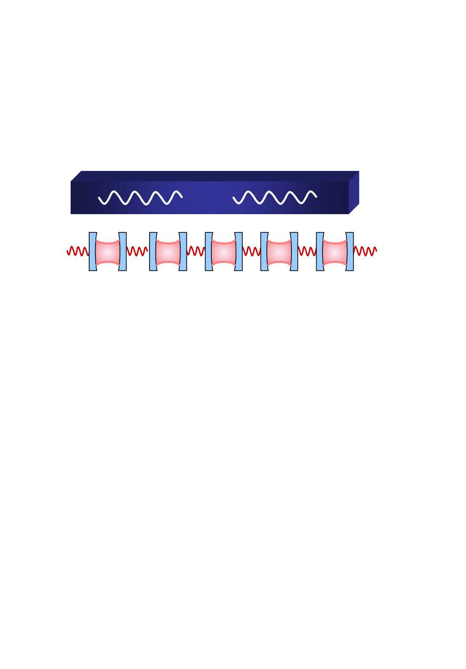
In the physical implementation, such kind of one-dimensional coupled resonator waveguide (CRW) can be realized by coupled superconducting transmission line resonators [17], coupled photonic-crystal microcavities or fibre-coupled toroidal microcavities. We will prove as follows that, for the “high energy” photons, the coupled resonator array will play the same role as that by the waveguide.
Usually, such nearest-neighbor interactions of cavities are modeled as a typical tight-binding coupling in terms of the creation and annihilation operators ( and ) of the modes localized in the th cavity. The model Hamiltonian for the CRW yields
| (3) |
where is the eigenfrequency of the cavity mode, and is the hopping constant between the neighboring sites. Here, the subscript index range from minus infinite to plus infinite.
The photonic spectrum of this CRW is continuous with its band extending from to . A propagating single photon in the CRW will occupy an energy
| (4) |
where is the momentum of the photon, and the lattice spacing is taken to be unit. In the low-energy regime , the long-wavelength approximation gives a quadratic spectrum
| (5) |
with , which is obtained by expanding the cosine function around zero. Then this system is reduced to the one that a particle with mass moves in a free space or a waveguide with no energy bound.
In the high-energy regime , the short-wavelength approximation leads to a linear spectrum
| (6) |
with , which is obtained by expanding the cosine function around .
III Quasi-spin wave excitations of atomic ensemble coupled to the photon hopping
In this section, we model the interaction between the hopping photons and the collective excitations of the atomic ensemble. Similar to the usual spin wave in the magnetic system, this collective excitation is described by a collective operator
| (7) |
where . Obviously, the above collective operators describe the collective excitation from the ground state with all atoms in the ground state. A single particle excitation is presented by . In the large limit, and under the low excitation condition that there are only a few atoms occupying the excited state , the collective operator satisfy the commutation relation
This means that the quasi-spin wave excitation is of bosonic type[18].
According to the reference [19], there also exist other collective modes, but they are decoupled with this mode by when the atoms is in the homogeneously broadening, i.e., all the energy level spacings are the same. Then the coupling between the atomic ensemble and the localized mode and in 0’th cavity reads
| (8) |
where the cavity mediated atom-photon coupling.
In terms of the quasi-spin-wave excitation of the atomic ensemble, the Hamiltonian in the low-energy regime reduces to
| (9) | |||||
In the high-energy regime, the Hamiltonian yields
| (10) | |||||
In the above equations, we have neglected constants terms, and the summation of over the atoms is inside a small but macroscopic volume around the position . Obviously, due to the cooperative motion of all atoms, the atom-photon interaction is enhanced by times. Thus our quantum node has a strong coupling to light, so that it can preform a fast control for the photon transfer.
IV Coherent scattering of photons by atomic ensemble
In this section, we consider the role of the enhanced coupling for the single photon transfer in the coupled resonator array. The strong coupling between the quasi-spin-wave and the cavity field leads to the emergence of dressed states of atoms by photons, which is called polaritons[20]. Polaritons are quasiparticles, which were introduced to reveal the physical mechanism for the temporary transfer of excitations to and from the medium many years ago[21, 22].
In our system, there are two polaritons, which are described by polariton operators
| (11a) | |||||
| (11b) | |||||
Here, the superpositions of the two operators and are defined by the angle
| (12) |
with the parameters
| (13) |
Obviously, polariton operators and still obey bosonic commutation relations.
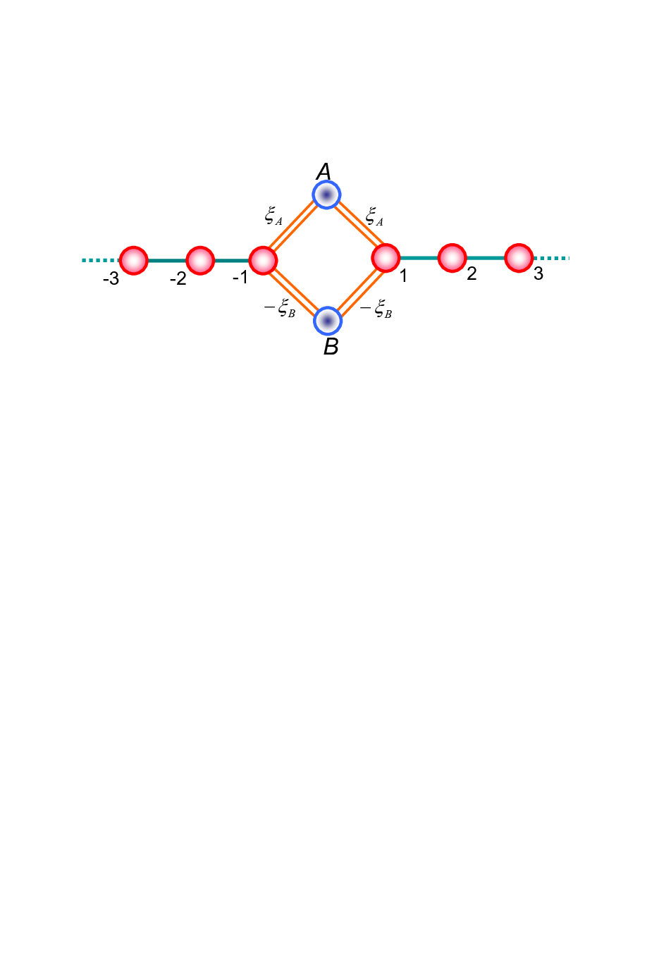
With quasi-particle operators and , the interaction between the atoms and the th cavity is diagonalized as
| (14) | |||||
where,
| (15) |
means that, in the atomic medium, the electromagnetic field will be split into two displacement vectors, which depicted by and respectively, corresponding to higher energy and lower energy .
In terms of the two dressed collective excitation operators and , we rewrite the total Hamiltonian
| (16) |
where and , which depends on the hopping constant respectively and represent the effective couplings of -polariton and -polariton to the hopping photons. This Hamiltonian describes a local two channel scattering process illustrated in Fig. 3 schematically. The energy difference between the two channel is determined by both the Jaynes-Cummings coupling constant and the numbers of atom in the unit volume, and so there exists an obvious -enhanced effects in the polariton split.
We confine ourselves to the single excitation subspace, since the total excitation number commutes with the Hamiltonian of the system. In the coordinator representation, the eigenstates in the single-excited subspace reads
| (17) |
where is the probability amplitude for finding the single photon at the th site, () is the probability amplitude of the single photon to localize at the th cavity by the formation of polaritons. The discrete Schrodinger equation gives the continuity of the wave functions in the scattering region around the atomic gas cell
| (18a) | ||||
| (18b) | ||||
| (18c) | ||||
| (18d) | ||||
V Photon transmission controlled by atomic ensemble
In this section, we study the photon scattering by the two polaritons through the above scattering equation in the discrete coordinate representation. Actually, the above equations (18) are the re-expression of the original discrete coordinate scattering equation first presented in Ref.[5]. All the results about the transmission and reflection with Fano line and Breit-Wigner line are valid in the present studies. To emphasize the role of the dressed states formed by atomic collective excitations coupled to the field of photon, we still apply the discrete coordinate equations (18) to calculate the transmission coefficient.

We assume an incoming wave within the CRW with energy , incident from the left, results in a reflected and transmitted wave. The wave functions in the asymptotic regions on the left and right are given by
| (19) |
By canceling the probability amplitude and in the boundary condition of Eq.(18), the transmission amplitude is obtained as
| (20) |
and the reflection amplitude also can be gotten by the relation .
We notice that the equation (20) is the same as that obtained in Ref.[5]. This point can be obviously seen by substituting the energy dispersive relation into Eq.(20). However, from the dressed state based representation in Eq.(20), the physical effects of photon scattering process can be feasibly explained with the two virtual channel pictures mentioned above. It can be observed from the above equations: i) transmission vanishes at the edge of band regardless of the location of energy level spacing, and these trivial zeros are caused by the vanishing group velocity at the ; ii) a vanishing transmission appears, once the energy level spacing is inside the energy band . Case two is related to the Fano resonance[23], which is the interference effect characterized by a certain discrete energy state interacting with the continuum. Indeed, as shown in Fig.4, the atomic ensemble provides the discrete energy state and the CRW provides the continuum here. It is the inside-band discrete state shown in Fig.4(a), which allows additional propagating path for the incident photon, and the destructive interference leads to perfect reflection.

All the above observations can be clearly seen in Fig.5. We compare Fig.5(d) three lines, the transmission probability gets much larger on the whole when the energy level spacing is tuned outside the band. The physical mechanism for this increasing transmission is schematically illustrated in Fig.4(b). In the scattering process when the energy level spacing is outside the band, the energy carried by the incident photon cannot excite quasi-spin-wave in the atomic ensemble, e.g. it occurs only a virtual exchange process of photons. However, since the atomic ensemble begins at the initial state with all atoms in a ground state and almost ended with the same state during the scattering process.
Let us understand the above increasing phenomenon of transmission from the point view of polaritons. The CRW on the left side of the th resonator forms a continuum with a propagation allowing bound , and so does the right side of the th resonator. The two continuum are connected by two discrete energy states at the point . These two discrete energy states correspond to the single quasi-particle excitation of different polaritons from the atomic-ensemble ground state . According to the previous definition in Eq.(15) and Eq.(14), the required energy for a single excitation of polariton is higher than that for a single excitation of polariton . Fig.5(a), (b) ,and(c) schematically shows the corresponding energy-level diagram. In Fig.5(a), the two energy levels of polariton are outside the band, the strong coupling removes both the single-excitated energy-level and the state of the resonator far away from the band, which almost blocks the tunneling process. Therefore the transmission is very small on the whole (see the Fig.5(d)’s a-line). When one of the polariton’s energy level is inside the band, there is some possibility for one discrete energy state inside the band just like Fig.5(b) and (c), which mediates the photonic hopping among the resonators. However, if the energy of one polariton approaches the middle of the band, the transmission probability becomes higher (see the Fig.5(d)’s b-line and c-line).
Finally let us come to the question which path will be taken with large probability in the scattering process of the single photon. Actually this question is answered intuitively in the discussion of the previous paragraph. We now give the relation between the single-photon scattering process and the probability for a photon to occur in the polaritons. From Eq.(18), the probability amplitude is obtained as
| (21a) | |||||
| (21b) | |||||
In Fig.6, we plot the probability and as the function of wave number . The read dash line presents the probability , and the blue solid line presents the probability . The parameters are taken as the same as Fig.5(d). In Fig.6(a), the atomic energy level spacing is inside the band. The case for outside the band is depicted in Fig.6(b,c).
In Fig.6(b), the atomic energy level spacing lies upper the band, while in Fig.6(b), lies below the band. It can been found that when is inside the band, and compare with each other. However, when the eigen-energy of the polariton is inside the band, as shown in Fig.5(b), there is a large probability for a single-photon to form the polariton at the point . Also when the energy level of polariton is inside the band, the probability becomes much larger, and becomes much smaller. Therefore, photon tends to form polariton rather than polariton .

The above observation can been understood from the difference between the coupling strength and . For the case shown in Fig.6(a), the coupling strength and approximately equal, therefore, compares with . However, in Fig.6(b,c), things become different. is much smaller than for the case shown in Fig.6(b), while for the case shown in Fig.6(c), the coupling strength is much smaller than . Therefore, by adjusting the energy level spacing of the atomic ensemble, one can choose the formation of polaritons in the th cavity.
VI Localized photons induced by polaritons
All the above arguments are based on the scattering approach with the discrete coordinate representation. In contrast to such delocalized states of scattering, there also exists the photon localization due to the formation of the polaritons, which are some quasi-particles described by the bound state. Actually, the bound state in continuum was first proposed in 1929 by von Neumann and Wigner[24]. From then on, there are so many studies to report its existence [25, 26, 27, 28, 29, 30]. The bound states are eigenstates of the whole system with some spatially localized properties. They are locally produced by lack of the periodicity in coordinator space and their corresponding eigenenergy is outside the energy band.
To find such bound state in our system, we return to the polariton free representation of scattering equation.
| (22) |
The above original Hamiltonian (22) is obviously equivalent to Eq. (16) with the polariton representation.
We assume
| (23) |
is a bound state with the site-dependent amplitude
| (24) |
Here, can be regarded the wave vector that connected with the energy by the dispersion relation for Bloch states.
The eigen-equation determines a set of discrete coordinator equations
| (25a) | ||||
| (25b) | ||||
which is the same as Eq.(18) with the polariton based representation.
As discovered in Refs.[5, 6], the above equations can be reduced into a scattering equation
| (26) |
with the effective potential
| (27) |
This local potential depend on the energy . It is crucial that this potential is resonant at the energy equal to the atomic energy level spacing . The resonance enhanced coupling to the Zero’th site will lead to a bound state with the imaginary momentum vector, so that being exponentially decay with is far away from the zero site.
This complex momentum vector can be determined by the equation
| (28a) | ||||
| (28b) | ||||
straightly formally given by Eq.(26). Then we obtain the transcendental equation for calculating the bound energy as
| (29) |
The above calculation gives the energy of the bound state as
| (30) |
When , and the energy , we can obtain only one the bound state energy satisfied all above requests from equation
| (31) |
We assume , and .
Considering Eq.(28b) and the energy is real, we obtain . So we can obtain complex momentum vector , that means it is one of the bound state. Similarly, when we can obtain the another bound state and it’s corresponding energy . We illustrate the bound state in the Fig.7(a) in the k-space and give the corresponding wave functions in the Fig.7(b) and Fig.7(c) respectively.
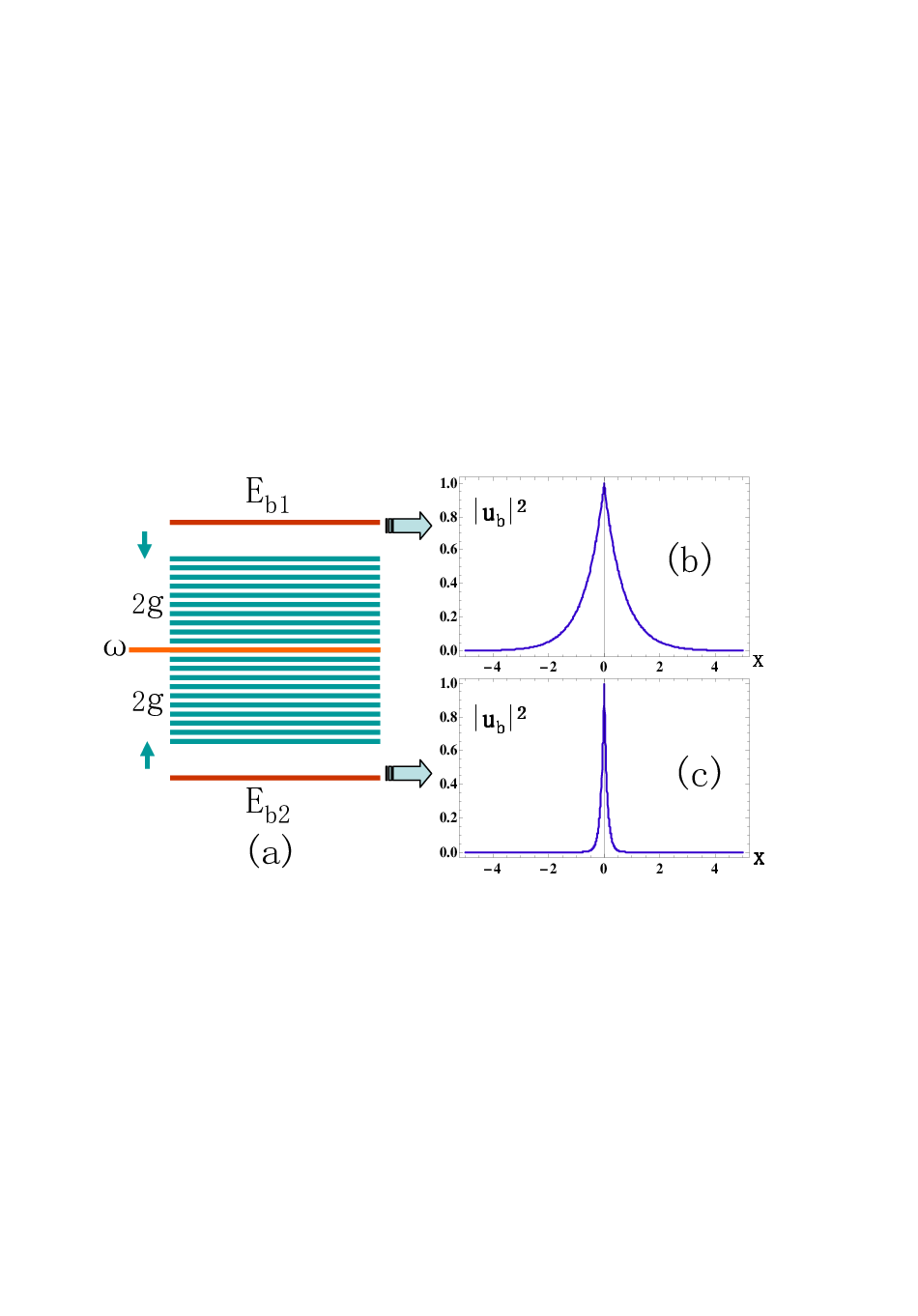
The above investigation display that there exist two localized single photon states with different energy.
VII Conclusion with a remarks
In summary, we have studied the scattering process of photons confined in a one dimensional optical waveguide by a laser controlled atomic ensemble. We show the possibility to bound single photon with an atomic ensemble based quantum node. Using the discrete coordinate approach, we exactly solve the effective scattering equations and gave the transmission rate of single photon in the coupled resonator array.
This investigation motivates us to proposed an active coherent control scheme for photon transferring in a waveguide by the localized atom ensemble. This construction can also create a local photon state called bound state. This finding implies a possibility to store the single photon state locally.
This work is supported by NSFC No. 90203018, No. 10474104, No. 60433050, No. 10325523, No. 10347128, No. 10075018 and No. 10704023, NFRPC No. 2006CB921205 and 2005CB724508, and the Scientific Research Fund of Hunan Provincial Education Department of China (Grant No. 07C579).
References
- [1] C. P. Sun, L. F. Wei, Y. X. Liu, and F. Nori, Phys. Rev. A 73, 022318 (2006).
- [2] D. E. Chang, A. S. Sørensen, E. A. Demler, and M. D. Lukin, Nat. Phys. 3, 807 (2007).
- [3] J. T. Shen and S. Fan, Phys. Rev. Lett. 95, 213001 (2005).
- [4] H. Dong, Z. R. Gong, H. Ian, L. Zhou, and C.P. Sun, arXiv:0805.3085.
- [5] L. Zhou, Z. R. Gong, Y. X. Liu, C. P. Sun, and F. Nori, Phys. Rev. Lett. 101, 100501 (2008).
- [6] Z. R. Gong, H. Ian, L. Zhou, and C. P. Sun, arXiv:0805.3042.
- [7] C. P. Sun, Y. Li, and X. F. Liu, Phys. Rev. Lett. 91, 147903 (2003).
- [8] Y. Li, and C. P. Sun, Phys. Rev. A 69, 051802 (2004).
- [9] M. D. Lukin, S. F. Yelin, and M. Fleischhauer, Phys. Rev. Lett. 84, 4232 (2000).
- [10] M. Fleischhauer and M. D. Lukin, Phys. Rev. Lett. 84, 5094 (2000).
- [11] D. F. Phillips, A. Fleischhauer, A. Mair, and R. L. Walsworth, Phys. Rev. Lett. 86, 783 (2001).
- [12] M. D. Lukin, Rev. Mod. Phys. 75, 457 (2003).
- [13] C. P. Sun, S. Yi, and L. You, Phys. Rev. A 67, 063815 (2003)
- [14] J. D. Joannopoulos, S. G. Johnson, J. N. Winn, and R. D. Meade, Photonic Crystals: Molding the Flow of Light (Princeton University Press, Princeton and Oxford, 2008).
- [15] Y. Xu, Y. Li, R. K. Lee, and A. Yariv, Phys. Rev. E 62, 7389 (2000).
- [16] F. M. Hu, L. Zhou, T. Shi, and C. P. Sun, Phys. Rev. A 76, 013819 (2007).
- [17] L. Zhou, Y.B. Gao, Z. Song, and C. P. Sun, Phys. Rev. A 77, 013831 (2008).
- [18] G. R. Jin, P. Zhang, Yu-xi Liu, and C. P. Sun, Phys. Rev. B 68, 134301 (2003).
- [19] Z. Song, P. Zhang, T. Shi, and C. P. Sun, Phys. Rev. B 71, 205314 (2005).
- [20] L. He, Y. X. Liu, S. Yi, C. P. Sun, and F. Nori, Phys. Rev. A 75, 063818 (2007).
- [21] S. M. Dutra and K. Furuya, Phys. Rev. A 55, 3832 (1997).
- [22] J. J. Hopfield, Phys. Rev. 112, 1555 (1958).
- [23] U. Fano, Phys. Rev. 124, 1866 (1961).
- [24] J. von Neumann and E. Wigner, Phys. Z. 30, 465 (1929).
- [25] F. H. Stillinger and D. R. Herrick, Phys. Rev. A 11, 446 (1975).
- [26] B. Gazdy, Phys. Lett. A 61, 89 (1977).
- [27] F. Capasso, C. Sirtori, J. Faist, D. L. Sivco, S.-N. G. Chu, and A. Y. Cho, Nature (London) 358, 565 (1992).
- [28] G. Ordonez, K. Na, and S. Kim, Phys. Rev. A 73, 022113 (2006).
- [29] H. Nakamura, N. Hatano, S. Garmon, and T. Petrosky, Phys. Rev. Lett. 99, 210404 (2007).
- [30] E. N. Bulgakov and A. F. Sadreev, Phys. Rev. B 78, 075105 (2008)