Critical behavior of loops and biconnected clusters on fractals of dimension $d<2$ .

Dibyendu Das Affiliation: Department of Physics, Indian Institute of Technology Bombay, Powai, Mumbai 400076, India Supravat Dey Affiliation: Department of Physics, Indian Institute of Technology Bombay, Powai, Mumbai 400076, India Jesper Lykke Jacobsen Affiliation: Laboratoire de Physique Théorique, Ecole Normale Supérieure, 24 rue Lhomond, 75321 Paris cedex 05, France Affiliation: Institut de Physique Th

\acute{e}

orique, CEA Saclay, 91191 Gif sur Yvette, France Deepak Dhar Affiliation: Department of Theoretical Physics, Tata Institute of Fundamental Research, Homi Bhabha Road, Mumbai - 400005, India

August 24, 2026

Abstract

We solve the O( $n$ ) model, defined in terms of self- and mutually avoiding loops coexisting with voids, on a $3$ -simplex fractal lattice, using an exact real space renormalization group technique. As the density of voids is decreased, the model shows a critical point, and for even lower densities of voids, there is a dense phase showing power-law correlations, with critical exponents that depend on $n$ , but are independent of density. At $n=-2$ on the dilute branch, a trivalent vertex defect acts as a marginal perturbation. We define a model of biconnected clusters which allows for a finite density of such vertices. As $n$ is varied, we get a line of critical points of this generalized model, emanating from the point of marginality in the original loop model. We also study another perturbation of adding local bending rigidity to the loop model, and find that it does not affect the universality class.

pacs

05.45.Df, 64.60.Ak, 05.50.+q, 64.60.Cn

I Introduction

The loop model is a very important model in statistical physics. It was defined originally in terms of the high temperature expansion of the $n$ -vector model [1, 2, 3]. The cases of $n=0,1,2$ correspond to well-studied cases of self-avoiding polymers [4], the critical Ising and the XY models [5], respectively. The model has been studied quite extensively in $d=2$ dimensions, in several variants, including fully packed or dilute versions, and with loops of more than one type. One can determine the critical exponents of the model on the hexagonal and square lattices using the Bethe Ansatz technique, the Coulomb gas method, and numerical techniques involving exact diagonalization of transfer matrices of systems on finite width cylinders [2, 3, 6, 7, 8, 9, 10]. The critical behavior of the model is also related to the dimer model, edge coloring model, compact polymer model (for $n\leq 2$ ) [11, 12, 10], and the hard hexagon model (for $n>2$ ) [13]. In the presence of a staggered field, the model gets related to the critical Potts model [14].

The loop model to be studied here is defined by the partition function

Z_{\rm loop}=\sum_{\cal C}n^{\cal L}\omega^{\cal V},

(1)

where the summation is over configurations ${\cal C}$ of self- and mutually-avoiding loops on a lattice. In the above, $n$ is the weight of a loop, $\omega$ is the weight of a vacancy (i.e., a lattice vertex not visited by any loop), ${\cal L}$ denotes the number of loops in a given configuration, and ${\cal V}$ the number of vacancies.

In Eq. (1), large values of $\omega$ correspond to a small average density of loops, and thus to the high-temperature phase of the $n$ -vector model. As $\omega$ is decreased, the average density of loops and the mean loop size increases, and diverges as $\omega$ tends to an $n$ -dependent critical value $\omega_{*+}(n)$ . The critical behavior of the loop model at $\omega_{*+}$ gives the critical behavior of the $n$ -vector model at its critical point in $d\geq 2$ . For $\omega<\omega_{*+}$ and $n\leq 2$ , the model shows a critical phase, which is called the dense phase. In $d=2$ , the critical exponents of the dense phase have been determined exactly [2, 7, 8, 9]. These vary with $n$ , but are independent of the precise value of $\omega$ .

The critical behavior of the loop model, and exponents of the dense phase have been less studied for $d\neq 2$ . One expects that the dense phase of the loop model for $d>2$ would be related to the the low-temperature phase of the $n$ -vector model. The latter shows power-law correlations in the entire low-temperature phase because of the existence of gapless Goldstone modes. In $d=2$ , Jacobsen et. al. [15] have shown that allowing loops to intersect or not leads to different critical behavior, and the dense phase of the loop model is different from the Goldstone phase.

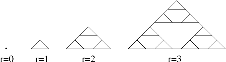
Refer to caption — Figure 1: The construction of the $3$ -simplex lattice is shown from level $r=0$ to $r=1$ and recursively for higher $r$ .

It therefore seems interesting to study the loop model in dimensions other than $d=2$ . In this paper, we study the loop model on fractal lattices with finite ramification index. We will take the $3$ -simplex lattice (see Fig. 1) as the simplest example of this type. The treatment is easily extended to other fractals. The loop model shows a nontrivial critical behavior for $n\leq 1$ on this fractal, and we determine the critical behavior near the dilute critical point $\omega_{*+}$ . We also study the critical properties of the dense phase. Further we define a generalization of the loop model, to be called the biconnected clusters model—or “bicon clusters model” for short—in which we allow the summation in the partition function to include all biconnected clusters, as shown in Fig. 2. A cluster is called bi-connected, iff between any two points of the cluster, there are at least two disjoint self-avoiding paths. Clearly all simple loops are biconnected. It turns out that this changes the critical behavior of the model, and we determine the new critical exponents.

A $d=2$ variant of the bicon model is known as the “net model” [16]. This model is relevant for the study of quantum models whose ground states are endowed with topological order. More generally, the constraint of $k$ -connectedness has also been imposed in classical models of clusters, such as percolation [17] and the Potts model [18].

There have been several studies of critical behavior of statistical mechanical systems on finitely ramified fractals [19]. The Ising model was the earliest to be studied on fractals [20]. It was followed by a study of self-avoiding polymers on a $3$ -simplex lattice [21]. Later self-interacting self-avoiding polymers [22], and other trails [23], have been studied. The Lee Yang edge singularity for Ising model was considered in [24]. The collapse transition of branched polymers was studied in [25]. The distribution of sizes of erased loops for loop-erased random walks was studied in [26]. In [27], it was studied how the number of self avoiding rings going through a site varies with the position of the site. Polymers with bending energy were studied on $3$ -simplex and other fractal lattices in [28]. For a recent review, see [29].

The detailed plan of the paper is as follows. In Section II we find the critical branches of the loop model, and in section III the exponents are calculated. In section IV we study the generalized “bicon model”, as mentioned above. In section V we study the loop model with extra energies for local bending. In section VI we summarize our results.

II The critical branches of the loop model

The recursive construction of the $3$ -simplex fractal lattice, through a series of levels $r$ , is illustrated in Fig. 1. Let $Z_{r}$ be the partition function at level $r$ , i.e. the sum of statistical weights of all configurations with loops contained within level $r$ , and denoted by an empty triangle in Fig. 3. We may have loops which close at levels higher than $r$ . Such a loop will come out of the corner vertices of an $r$ -th level triangle. The restricted partition function for configurations with such an open chain passing out of the corner vertices of a $r$ -th level triangle is denoted by $B_{r}$ and shown in Fig. 3.

These functions $Z_{r}$ and $B_{r}$ can be recursively related to their counterparts at the $(r+1)$ -th level by the following equations:

	$\displaystyle Z_{r+1}={Z_{r}}^{3}+n{B_{r}}^{3}$		(2)
	$\displaystyle B_{r+1}=Z_{r}{B_{r}}^{2}+{B_{r}}^{3}.$		(3)

At the $0$ -th level the lattice has just a single site. In that case $Z_{0}=\omega$ is the weight of it being empty, and $B_{0}=1$ is the weight that a loop passes through it. If we define $\omega_{r}=Z_{r}/B_{r}$ , then the recursion relation for the latter is

\displaystyle\omega_{r+1}=\frac{\omega_{r}^{3}+n}{\omega_{r}+1}.

(4)

At the $0$ -th level, $\omega_{0}=Z_{0}/B_{0}=\omega$ . The total free energy on an infinite lattice is

\displaystyle F(n,\omega)

\displaystyle=

\displaystyle\lim_{r\rightarrow\infty}\frac{1}{3^{r}}~{\rm ln}~Z_{r+1}.

(5)

Eq. (5) above may be rewritten, using $Z_{r+1}=Z_{r}^{3}(Z_{r+1}/Z_{r}^{3})$ , and after a little algebra we obtain

\displaystyle F(n,\omega)=\frac{1}{3}{\rm ln}(1+n{\omega}^{-3})+\frac{1}{3}F\left(n,\frac{\omega^{3}+n}{\omega+1}\right),

(6)

which is the usual form [30] of the recursion relation for the free energy under the real-space renormalization group (RG). Apart from $\omega_{*}=\infty$ , the finite-valued fixed points of the RG flow (4) are the roots of the following equation:

\omega_{*}^{3}-\omega_{*}^{2}-\omega_{*}+n=0.

(7)

The special case $n=0$ corresponding to self-avoiding polymers was studied earlier [21].

Eq. (7) has three real solutions for $-5/27\leq n\leq 1$ , and only one real solution for the regions $n>1$ and $n<-5/27$ (see Fig. 4). The three fixed points for the region $-5/27\leq n\leq 1$ are given by the formulae

	$\displaystyle\omega_{*}$	$\displaystyle=$	$\displaystyle\frac{1}{3}\left(1+4\cos\left(\frac{\theta}{3}\right)\right),$		(8)
	$\displaystyle n$	$\displaystyle=$	$\displaystyle\frac{1}{27}\left(11-16\cos(\theta)\right),$		(9)

where $\theta\in[0,3\pi]$ . The three solutions correspond to the following subdivision of the parameter range of $\theta$ :

•

For $\theta\in[0,\pi]$ , $n$ runs from $-5/27$ to $1$ , and $\omega$ from $5/3$ to $1$ . We shall refer to this line of fixed points as the dilute branch and denote it by $\omega_{*+}(n)$ . It is physical ( $n\geq 0$ ) for $\theta\geq\cos^{-1}(11/16)\simeq 0.8128$ .
•

For $\theta\in[\pi,2\pi]$ , $n$ runs from $1$ to $-5/27$ , and $\omega$ from $1$ to $-1/3$ . We shall refer to this as the dense branch and denote it by $\omega_{*-}(n)$ . It is physical ( $n\geq 0$ and $\omega\geq 0$ ) for $\theta\leq 2\pi-\cos^{-1}(11/16)\simeq 5.4704$ .
•

For $\theta\in[2\pi,3\pi]$ , $n$ runs from $-5/27$ to $1$ , and $\omega$ from $-1/3$ to $-1$ .

This unphysical critical point at negative $\omega$ may be called the Yang Lee edge singularity in our problem. We shall denote it by $\omega_{YL}$ . However, we note that the critical behavior at this ”Yang Lee edge singularity” is not independent of $n$ .

The three branches $\omega_{*+}$ , $\omega_{*-}$ and $\omega_{YL}$ are shown in figure 4. Note that unlike the two-dimensional loop model, where the critical region between the dilute and dense branches extends up to $n=2$ , the domain of criticality of the present model is smaller. But here too, the upper branch is a repulsive fixed line. Starting from any $\omega>\omega_{*+}$ the RG flows take one to $\omega=\infty$ while starting from any $\omega<\omega_{*+}$ the lower branch $\omega_{*-}(n)$ serves as a line of attraction of the RG flow. We will refer to the region with $\omega<\omega_{*+}$ as the dense phase.

For $n<-5/27$ , the dilute branch can be extended backwards by replacing $\theta=i{\tilde{\theta}}$ (with ${\tilde{\theta}}\in[0,\infty)$ ), i.e replacing “ $\cos$ ” by “ $\cosh$ ” and $\theta$ by ${\tilde{\theta}}$ in Eqs. (8) and (9). Although this regime is unphysical, we will show in section III.4 that the point $(n=-2,\omega=2)$ on it is of some signficance.

For $n>1$ , the nontrivial fixed point other than $\omega_{*}=\infty$ is negative, and is obtained by replacing $\theta=3\pi+i{\tilde{\theta}}$ (with ${\tilde{\theta}}\in[0,\infty)$ ), i.e. replacing “ $\cos$ ” by “ $-\cosh$ ” and $\theta$ by ${\tilde{\theta}}$ in Eqs. (8) and (9). There is no nontrivial critical point for positive $\omega$ . It can be shown [31] that the loop model for $n=2$ can be exactly mapped to a weighted $6$ -vertex model, which also can have no nontrivial critical point for positive weights in this regime.

III The exponents of the loop model

In two dimensions, for a generic point lying on the dilute branch or in the dense phase, the loop model is known to have an infinite set of exponents characterizing its critical behaviour [12, 32]. The full set of principal exponents consists of an infinite number of correlation exponents associated with defects called the $k$ -string defects, plus one thermal exponent.

A $k$ -string defect has an integer $k(\geq 1)$ number of “open chains” originating from a local neighborhood and terminating in an anti-defect very far away. Since chains are disallowed in the original loop model, such structures may be imagined to be created in isolation, as defects, upon application of suitable small external fields. A closed loop with two points marked on it is equivalent to a $2$ -string defect, and this observation can be used [12, 32, 14] to find the fractal dimension of the closed loops in the loop model. Although there is no upper bound on $k$ for ordinary Euclidean lattices, on fractals due to finite ramification, the exponent spectrum becomes finite. For the present model on the $3$ -simplex fractal lattice we can have such defects only with $k\leq 3$ . [On the Sierpinski gasket, one could have $k\leq 4$ .]

Apart from the $k$ -string defects, the loop model also has the thermal defect and different exponents associated with it, namely the specific heat exponent, the correlation length exponent, etc. Among the latter only one is independent and others can be related to it by identities. Thus there are four independent exponents for the loop model on the $3$ -simplex lattice, three $k$ -string exponents plus one thermal exponent, and we calculate them in the following subsections III.1-III.4.

III.1 The exponents related to thermal excitation

Let us define $(\omega-\omega_{*+})$ as the “thermal distance” from the critical point $\omega_{*+}$ . Starting from $\omega_{0}=\omega>\omega_{*+}$ , under succesive iteration of Eq. (4), the separation $\delta_{r}=(\omega_{r}-\omega_{*+})$ increases with increasing $r$ . We note that $\delta_{0}=(\omega-\omega_{*+})$ . Using Eqs. (4) and (7), we easily find that $\delta_{r}=\lambda_{T}^{r}\delta_{0}$ with

\displaystyle\lambda_{T}=\left(\frac{3-\omega_{*+}^{-1}}{1+n\omega_{*+}^{-3}}\right).

(10)

The thermal exponent $y_{T}$ is defined as usual by the fact that at the $r$ -th step of RG transformation, the thermal distance $\delta_{r}\sim(2^{y_{T}})^{r}\delta_{0}$ . Thus comparing the two expressions for $\delta_{r}$ we obtain

\displaystyle y_{T}=\frac{\ln{\lambda_{T}}}{\ln{2}}

(11)

The specific heat exponent $\alpha$ may be defined via the scaling behavior of the non-analytic part of the free energy, namely $F\sim(\omega-\omega_{*+})^{2-\alpha}$ . Substituting the latter scaling form into Eq. (6) and comparing the singular terms, a straightforward calculation yields

\displaystyle\alpha=2-\frac{\ln 3}{\ln\lambda_{T}},

(12)

where $\lambda_{T}$ is given by Eq. (10).

Thermal fluctuations create thermal defects and the correlation function $C({\bf R})$ for two such defects separated by distance $|{\bf R}|$ is defined for $\omega>\omega_{*+}$ as

\displaystyle C({\bf R})=\frac{1}{|{\bf R}|^{c}}f\left(\frac{|{\bf R}|}{\xi}\right).

(13)

The correlation length $\xi$ is finite for $\omega>\omega_{*+}$ and the scaling relation $\xi\sim(\omega-\omega_{*+})^{-\nu}$ defines the correlation length exponent $\nu$ . Under RG, if $\xi\sim b$ , since $(\omega-\omega_{*+})\sim b^{-y_{T}}$ it follows immediately that

\displaystyle\nu=1/y_{T}=\frac{\ln 2}{\ln\lambda_{T}}.

(14)

For $\omega=\omega_{*+}$ , in Eq. (13), $\xi\rightarrow\infty$ and $c=2x_{T}$ , where $x_{T}$ is called the thermal correlation exponent at criticality. From standard RG arguments [30] it can be shown that $x_{T}=d-y_{T}$ , where

\displaystyle d=\frac{\ln 3}{\ln 2}

(15)

is the box dimension of the $3$ -simplex fractal lattice. From Eqs. (12) and (14) we see that the hyperscaling relation $d\nu=2-\alpha$ holds.

Apart from the exponents of thermal origin discussed above, there are several other exponents caracterizing the behavior of other physically interesting observables, which can be expressed in terms of the exponents described above:

•

The fractal dimension of the loops given by $d_{f}$ relates the length $s$ and radius $R$ of a loop as $s\sim R^{d_{f}}$ . The exponent $d_{f}$ is distinct for the two critical regions $\omega=\omega_{*+}$ (dilute branch) and $\omega<\omega_{*+}$ (dense phase). We show in section III.3 that they can be easily related to the $2$ -string correlation exponent $x_{2}$ .
•

For $\omega>\omega_{*+}$ , the distribution of loop sizes $s$ has an exponential cutoff $\sim\exp(-as)$ . The cutoff length $a^{-1}\sim\xi^{d_{f}}$ , where $\xi$ is the finite correlation length in the disordered phase. One can find $a^{-1}$ as in the derivation of $\nu$ above.
•

For the critical regimes $\omega=\omega_{*+}$ and $\omega<\omega_{*+}$ , the probability distribution of loop size $s$ is an unbounded power law $\sim s^{-({\tau-1})}$ . The exponent $\tau$ is distinct for $\omega=\omega_{*+}$ and $\omega<\omega_{*+}$ , and it is easy to express the exponent $\tau$ in terms of the exponents $x_{2}$ and the fractal dimension $d_{f}$ of the loops (see section III.3).

The exponents like $d_{f}$ and $\tau$ can all be expressed in terms of the “ $k$ -string defect” exponents which we derive in the following three subsections.

III.2 A $1$ -string defect

Let the application of a small external magnetic field $h_{1}$ create an open chain, or a $1$ -string defect, with the magnetic scaling exponent $y_{1}$ associated with it. Assuming for $h_{1}=0$ the system is critical, a finite $h_{1}$ introduces a finite correlation length $\xi$ given by

\displaystyle\xi(h_{1})\sim h_{1}^{-{1/y_{1}}}.

(16)

Eq. (16) defines the scaling exponent $y_{1}$ . In real space RG, upon coarse-graining from level $r$ to level $(r+1)$ , $\xi$ increases by a factor of $2$ , while $h_{1}$ increases by a factor of $\lambda_{1}$ , i.e. $\xi(h_{1})=2\xi(\lambda_{1}h_{1})$ . Below, we will calculate $\lambda_{1}$ , and using this with Eq. (16), one gets

\displaystyle y_{1}=\frac{\ln\lambda_{1}}{\ln 2}.

(17)

The probability $G({\bf X-Y})$ [32] of $k$ strings originating at ${\bf X}$ and ending at ${\bf Y}$ in the critical phase is given by

\displaystyle G({\bf X-Y})\sim 1/|{\bf X}-{\bf Y}|^{2x_{k}}.

(18)

¿From standard RG analysis it is known [30] that the correlation exponent $x_{k}$ is related to $y_{k}$ via the relation:

\displaystyle x_{k}=d-y_{k}.

(19)

Thus for our $1$ -string defect, by using Eq. (17) and box dimension (15), we get

\displaystyle x_{1}=d-y_{1}=\frac{\ln(3/\lambda_{1})}{\ln 2}.

(20)

Now we proceed to obtain the scale factor $\lambda_{1}$ . First we note that an $1$ -string defect may have its one endpoint inside an $r$ -th level triangle. The corresponding restricted partition functions $A_{r}$ and $C_{r}$ are represented by diagrams $A$ and $C$ in Fig. 3. The recursion relations for ${\tilde{A}}_{r}=A_{r}/Z_{r}$ , ${\tilde{C}}_{r}=C_{r}/Z_{r}$ , and ${\tilde{D}}_{r}=D_{r}/Z_{r}$ are as follows:

$\displaystyle{\tilde{A}}_{r+1}$	$\displaystyle=$	$\displaystyle\frac{{{\tilde{A}}_{r}}(1+2\omega^{-1}_{r}+2{\omega^{-2}_{r}})+{{\tilde{C}}_{r}}{\omega^{-2}_{r}}(n+2)}{1+n{\omega^{-3}_{r}}}$	(21)
$\displaystyle{\tilde{C}}_{r+1}$	$\displaystyle=$	$\displaystyle\frac{({\tilde{A}}_{r}+3{\tilde{C}}_{r}){\omega^{-2}_{r}}}{1+n{\omega^{-3}_{r}}}$	(22)
$\displaystyle{\tilde{D}}_{r+1}$	$\displaystyle=$	$\displaystyle\frac{{{\tilde{A}}_{r}}^{2}+{{\tilde{C}}_{r}}^{2}\omega^{-1}_{r}(n+6)+4{\tilde{A}}_{r}\omega^{-1}_{r}{\tilde{C}}_{r}+2{{\tilde{A}}_{r}}^{2}\omega^{-1}_{r}+{\tilde{D}}_{r}(2\omega^{-1}_{r}+3{\omega^{-2}_{r}})}{1+n{\omega^{-3}_{r}}}$	(23)

We can linearize Eqs. (21)–(22) around the fixed point $(A^{*},C^{*},D^{*})=(0,0,0)$ , and we are left with the matrix

\displaystyle\left[\begin{array}[]{cc}a+2&~~a(n+2)\omega_{*}^{-2}\\ &\\ a\omega_{*}^{-2}&~~3a\omega_{*}^{-2}\\ \end{array}\right]

with $a=1/(1+n\omega_{*}^{-3})$ . The largest eigenvalue of the matrix is $\lambda_{1}$ and is given by

\displaystyle\lambda_{1}=\frac{1}{2\omega_{*}^{2}}\left(3a+\omega_{*}^{2}(a+2)+\sqrt{a^{2}(17+4n)-6a\omega_{*}^{2}(a+2)+\omega_{*}^{4}(a+2)^{2}}\right).

(28)

Note that in Eq. (28), $\omega_{*}$ must be replaced by $\omega_{*+}$ or $\omega_{*-}$ in order to describe the dilute or dense branch, respectively. Using Eq. (28), we may thus write ${\tilde{A}}_{r}\sim\lambda_{1}^{r}{\tilde{A}}_{0}$ . It is clear that $A_{0}$ is proportional to the small external field $h_{1}$ , and thus using Eq. (28), we may read off the values of $y_{1}$ and $x_{1}$ in Eqs. (17) and (20).

Another exponent of interest is $\gamma_{1}$ associated with the approach from above of the dilute critical branch. It is defined via the scaling behavior of the average open chain length $\langle l_{1}\rangle\sim(\omega-\omega_{*+})^{-\gamma_{1}}$ . In general,

\displaystyle\langle l_{1}\rangle=\lim_{N\rightarrow\infty}\frac{1}{N}\sum_{n=1}^{\infty}{c_{n}p_{n}},

(29)

where $c_{n}$ is the number of distinct configurations each with an open chain length $n$ in a lattice of size $N$ , and $p_{n}$ is the relative weight factor for such a configuration normalized by the partition function. On our fractal lattice, this becomes

	$\displaystyle\langle l_{1}\rangle$	$\displaystyle=$	$\displaystyle\sum_{r=1}^{\infty}\frac{1}{3^{r}}\left(\frac{f_{r}}{Z_{r}}\right)$		(30)
		$\displaystyle=$	$\displaystyle\sum_{r=1}^{\infty}\frac{1}{3^{r}}\frac{\left(3{\tilde{A}}_{r-1}^{2}+3\omega^{-1}_{r-1}{\tilde{A}}_{r-1}^{2}+3\omega^{-2}_{r-1}{\tilde{D}}_{r-1}\right)}{\left(1+n\omega^{-3}_{r-1}\right)},$		(30)

where the statistical weight of fully containing an open chain at the $(r+1)$ th level is $f_{r+1}=3A_{r}^{2}Z_{r}+3B_{r}A_{r}^{2}+3B_{r}^{2}D_{r}$ . For a fixed and small distance from the critical point $\delta_{0}=(\omega-\omega_{*+})$ , since $\langle l_{1}\rangle$ is finite, the sum in Eq. (30) is sharply cut off at some finite level $r=r_{0}$ . We note that for $r>r_{0}$ , ${\tilde{A}}_{1,r}\sim\lambda_{1}^{r_{0}}$ , and ${\tilde{D}}_{r}\sim\lambda^{2r_{0}}$ , and $\delta_{0}\sim({\rm constant})/\lambda_{T}^{r_{0}}$ (see Eq. (10)). It immediately follows from the scaling relation $\langle l_{1}\rangle\sim{\delta_{0}}^{-\gamma_{1}}$ that

\gamma_{1}=\frac{\ln({\lambda^{2}}/3)}{\ln\lambda_{T}}.

(31)

As a check of consistency, we may verify the following exponent equality [32], using Eqs. (31), (20) and (14),

\displaystyle\gamma_{1}=(d-2x_{1})\nu.

(32)

III.3 A $2$ -string defect

Let a triangle at the $r$ -th level which has endpoints of $2$ -strings on two neighboring sites inside it, be defined to have a statistical weight $D^{{}^{\prime}}_{r}$ . Note that this weight is different from $D_{r}$ (see section III.3 above), since the latter puts no restriction on the location of the endpoints. Further defining ${\tilde{D}}^{{}^{\prime}}=D^{{}^{\prime}}/Z$ , we easily see that its recursion equation is

\displaystyle{\tilde{D}}^{{}^{\prime}}_{r+1}=\frac{2\omega^{-1}_{r}+3\omega^{-2}_{r}}{1+n\omega^{-3}_{r}}~{\tilde{D}}^{{}^{\prime}}_{r}.

(33)

Replacing $\omega_{r}$ with the fixed point value $\omega_{*}$ in the above equation, we get ${\tilde{D}}^{{}^{\prime}}_{r}\sim\lambda_{2}^{r}{\tilde{D}}^{{}^{\prime}}_{0}$ , with

\displaystyle\lambda_{2}=\frac{2{\omega_{*}}^{-1}+3{\omega_{*}}^{-2}}{1+n{\omega_{*}}^{-3}}=\frac{2{\omega_{*}}+3}{\omega_{*}+1},

(34)

where we have used Eq. (7). Note again that in Eq. (34) for $\lambda_{2}$ we have to use $\omega_{*}=\omega_{*+}$ for the upper branch, and $\omega_{*}=\omega_{*-}$ for the lower branch. If a small field $h_{2}$ creates a $2$ -string defect and the finite correlation length arising due to it is $\xi(h_{2})\sim h_{2}^{-{1/y_{2}}}$ , we find that the scaling exponent $y_{2}$ for a $2$ -string defect is

\displaystyle y_{2}={{\rm ln}\lambda_{2}}/{{\rm ln}2}.

(35)

¿From Eq. (19) we conclude that the corresponding correlation exponent $x_{2}$ is given by

\displaystyle x_{2}=d-y_{2}.

(36)

It is important to note that $y_{2}$ is also the fractal dimension $d_{f}$ of the loops. This is explicitly seen as follows. Let $l_{r}$ be the typical length of a segment of a loop that goes from one corner vertex to another in one $B$ -type triangle (see Fig. 3) of order $r$ . Then the typical length of a loop which closes at the $(r+1)$ -th level is $s_{r}=3l_{r}$ . The recursion for $l_{r}$ is:

\displaystyle l_{r+1}=\left(\frac{2Z_{r}B_{r}^{2}+3B_{r}^{3}}{Z_{r}B_{r}^{2}+B_{r}^{3}}\right)l_{r}.

(37)

The above Eq. (37) follows from the fact that at level $(r+1)$ , a typical loop length $l_{r+1}$ can be made of two $l_{r}$ segments with statistical weight $Z_{r}B_{r}^{2}/B_{r+1}$ , or three $l_{r}$ segments with statistical weight $B_{r}^{3}/B_{r+1}$ [33]. On the other hand, the typical diameter $R_{r}$ of such a segment of length $l_{r}$ is given by $R_{r}\sim 2^{r}$ . Combining these two results and using the definition of $d_{f}$ given by the scaling behavior $s_{r}\sim l_{r}\sim R_{r}^{d_{f}}$ , we conclude that

\displaystyle d_{f}=\frac{\ln\lambda_{2}}{\ln 2}=y_{2}.

(38)

We note that $d_{f}$ , through $\lambda_{2}$ , is distinct for $\omega_{*}=\omega_{*+}$ (dilute loops) and $\omega_{*}=\omega_{*-}$ (dense loops). For $n=0$ and in the dense loop phase, $\lambda_{2}=3$ , and so $d_{f}$ coincides with the box dimension $d$ of Eq. (15). This was to be expected, since the limit of dense loops ( $\omega_{*-}\to 0$ ) in fact means that there is a single loop covering the entire lattice, i.e., the loop is Hamiltonian. For dilute loops, we have $\omega_{*+}=\frac{1}{2}(1+\sqrt{5})$ , whence $\lambda_{2}=\frac{1}{2}(7-\sqrt{5})$ and $d_{f}\simeq 1.2522$ .

The probability distribution $P(s)$ of loop size $s$ is an unbounded power law $\sim s^{-({\tau-1})}$ for both the dilute branch and the dense phase. The exponent $\tau$ can be related to $x_{2}$ and $d_{f}$ following a general derivation as in [34]. Let $G_{s}({\bf R})$ be the probability that two points separated by ${\bf R}$ are on a loop of size $s$ . The expected scaling form of $G_{s}({\bf R})$ is:

\displaystyle G_{s}({\bf R})\sim s^{m}|{\bf R}|^{-c_{1}}f_{1}\left(\frac{|{\bf R}|}{s^{1/d_{f}}}\right).

(39)

Firstly, the sum of $G_{s}({\bf R})$ over all the space, i.e. $\int d^{d}{\bf R}G_{s}({\bf R})$ , is nothing but number of points on the loop $=s$ . This gives a relation $d-c_{1}=d_{f}(1-m)$ . Secondly, by definition (see Eq. (18)) we have $G({\bf R})=\int dsP(s)G_{s}({\bf R})\sim|{\bf R}|^{-2x_{2}}$ . The latter relation combined with the former gives

\displaystyle d_{f}(3-\tau)=d-2x_{2},

(40)

which is the desired result.

III.4 A $3$ -string defect:

Let a triangle at the $r$ -th level which has endpoints of $3$ -strings on three neighbouring sites inside it, be defined to have a statistical weight $E^{{}^{\prime}}_{r}$ . The recursion relation of ${\tilde{E}}^{{}^{\prime}}=E^{{}^{\prime}}/Z$ is

\displaystyle{\tilde{E}}^{{}^{\prime}}_{r+1}=\frac{3\omega^{-2}_{r}}{1+n\omega^{-3}_{r}}~{\tilde{E}}^{{}^{\prime}}_{r}.

(41)

Assuming that a small field $h_{3}$ creates a $3$ -string defect and the corresponding finite correlation length $\xi(h_{3})\sim h_{3}^{-{1/y_{3}}}$ , we find that

\displaystyle y_{3}={{\rm ln}\lambda_{3}}/{{\rm ln}2},

(42)

where

\displaystyle\lambda_{3}=\frac{3\omega_{*}}{\omega_{*}^{3}+n}.

(43)

The correlation exponent $x_{3}$ corresponding to $y_{3}$ is given by Eq. (19) with $k=3$ .

We now note something very interesting. If we extend the upper dilute critical branch to negative values of $n<-5/27$ , we find that at the special point $(\omega_{*}=2,n=-2)$ , we have $\lambda_{3}=1$ and $y_{3}=0$ (see eqs. (42) and (43)). Thus although the $1$ -, $2$ - and $3$ -string defects are relevant for general $n$ on both the critical branches, at the point $(\omega_{*}=2,n=-2)$ the $3$ -string defect becomes marginal. In the next section IV, we define a more general model called the “biconnected cluster model” which allows for vertices of degree 3, each occuring with a finite weight $\omega_{3}$ . We find that the latter model has a new critical line in its larger parameter space, which precisely meets with the line of critical points corresponding to $\omega_{3}=0$ at the point $(\omega_{*}=2,n=-2)$ on the extended dilute branch.

IV The biconnected cluster model

The finding in section III.4 that $y_{3}=0$ at a point in the $(\omega,n)$ parameter space, motivates our study of a model called the biconnected cluster model in which the allowed vertex degrees are 0, 2 and 3. In other words, $3$ -strings are allowed to emerge from any vertex (see Fig. 5(a)). The connected components are further required to be 2-connected, i.e., they cannot be disconnected upon cutting a single link (see Fig. 5(b))—note that this is a stronger requirement than simply disallowing vertices of degree 1. Henceforth we will refer to this model as the “bicon clusters model”, to distinguish it from the “loop model” studied this far in the paper. A similar model—with no requirement of biconnectedness—was studied in two dimensions in [16] under the name of “net model”. The partition sum for the bicon model is

Z_{\rm bicon}=\sum_{\cal C}n^{\cal L}\omega^{\cal V}\omega_{3}^{\cal U},

(44)

where the summation is over configurations ${\cal C}$ of any number of self-, and mutually-avoiding biconnected clusters. Here $n$ is the weight of a cluster of any size, $\omega$ is the weight of an empty vertex, and $\omega_{3}$ is the weight of a vertex of degree 3. Further, ${\cal L}$ denotes the number of clusters, ${\cal V}$ the number of vacancies, and $\cal U$ the number of vertices of degree $3$ , in a given configuration. Note that by setting $\omega_{3}=0$ , the bicon clustes model reduces to the usual loop model. Some of the configurations that we exclude from the model (see Fig. 5(b) for an example) will be treated as defect configurations called “ $k$ -defects” in section IV.2 below.

The three possible vertex configurations with weights $\omega$ , $1$ and $\omega_{3}$ are shown in Fig. 6. Note that if ${\cal N}_{k}$ is the number of vertices of degree $k$ , we have the simple topological identity $2{\cal N}_{2}+3{\cal N}_{3}=2L$ , where $L$ is the total number of links in the configuration. Therefore ${\cal N}_{3}={\cal U}$ is necessarily even. Accordingly, the bicon clusters model partition function is a function of $(\omega_{3})^{2}$ . At the $r$ -th level, the real space RG closes for three restricted partition functions schematically shown as $Z$ , $F$ and $G$ in Fig. 6. While $Z_{r}$ is the partition function summing over configurations with no strings coming out of the corner vertices, $F_{r}$ and $G_{r}$ have two and three strings coming out of the corners, respectively. Note that the constraint of biconnectedness implies that it is not possible to have a configuration with one string coming out of the corner vertices. At the level $r=0$ ,

\displaystyle Z_{0}=\omega;~~F_{0}=1;~~G_{0}=\omega_{3}.

(45)

At the $r$ -th level, the recursion relations are:

$\displaystyle Z_{r+1}$	$\displaystyle=$	$\displaystyle Z_{r}^{3}+nF_{r}^{3}$	(46)
$\displaystyle F_{r+1}$	$\displaystyle=$	$\displaystyle F_{r}^{3}+F_{r}^{2}Z_{r}+F_{r}G_{r}^{2}$	(47)
$\displaystyle G_{r+1}$	$\displaystyle=$	$\displaystyle G_{r}^{3}+3G_{r}F_{r}^{2}$	(48)

Further defining ${\tilde{F}}_{r}=F_{r}/Z_{r}$ , and ${\tilde{G}}_{r}=G_{r}/Z_{r}$ , we get

	$\displaystyle{\tilde{F}}_{r+1}$	$\displaystyle=$	$\displaystyle\frac{{\tilde{F}}_{r}^{3}+{\tilde{F}}_{r}^{2}+{\tilde{F}}_{r}{\tilde{G}}_{r}^{2}}{1+n{\tilde{F}}_{r}^{3}}$		(49)
	$\displaystyle{\tilde{G}}_{r+1}$	$\displaystyle=$	$\displaystyle\frac{{\tilde{G}}_{r}^{3}+3{\tilde{G}}_{r}{\tilde{F}}_{r}^{2}}{1+n{\tilde{F}}_{r}^{3}}$		(50)

Note that ${\tilde{F}}_{0}=\omega^{-1}$ and ${\tilde{G}}_{0}=\omega_{3}\omega^{-1}$ . There are several fixed points $({\tilde{F}}_{*},{\tilde{G}}_{*})$ of Eqs. (49)–(50). Apart from the trivial weak coupling fixed point $(0,0)$ and the fixed point $(\infty,\infty)$ corresponding to all bonds being fully covered, there are the dilute and dense fixed points of the loop model which we denote by $({\tilde{F}}_{+},0)$ and $({\tilde{F}}_{-},0)$ , respectively. But most importantly there is a nontrivial fixed point $({\tilde{F}}_{*},{\tilde{G}}_{*})$ given by,

\displaystyle{\tilde{F}}_{*}=1/2~~~{\rm and}~~~{\tilde{G}}_{*}=\sqrt{\frac{1}{4}+\frac{n}{8}}.

(51)

The latter defines a new critical line in the $(\omega,n,\omega_{3})$ space, which terminates on one end at the point $(\omega=2,n=-2,\omega_{3}=0)$ ; note that this is the point where we found $y_{3}$ to be marginal for the loop model in section III.4. The dense-phase fixed point $({\tilde{F}}_{-},0)$ is unstable to introduction of trivalent sites, and the limiting behaviour of the critical net model is governed by the fixed point $({\tilde{F}}_{*},{\tilde{G}}_{*})$ .

If the starting value of ${\tilde{F}}_{r}$ and ${\tilde{G}}_{r}$ is near ${\tilde{F}}_{*}$ and ${\tilde{G}}_{*}$ , but a bit larger, it is easy to check that ${\tilde{F}}_{r}$ and ${\tilde{G}}_{r}$ diverge to infinity as $r$ and $r^{3/2}$ respectively. This implies that in the dense phase of the bicon clusters models, corner sites of triangles of high order belong to the infinite cluster with a large probability, and this probability tends to $1$ as $r$ tends to infinity.

IV.1 The fractal dimension of the biconnnected clusters

Just like in the loop model, we would like to find the fractal dimension of the clusters in the bicon clusters model at its critical point. Consider two marked points $A$ and $B$ on a cluster, free of tadpole overhangs. Imagine that these marks are “defects” created by some external field $h$ . In addition to $F$ and $G$ , we now define new functions $F^{m}$ and $G^{m}$ which are analogous to $F$ and $G$ , except that they represent configurations in which there is exactly one marked point. At level $r=0$ we have:

	$\displaystyle F_{0}^{m}$	$\displaystyle=$	$\displaystyle h$
	$\displaystyle G_{0}^{m}$	$\displaystyle=$	$\displaystyle h\omega_{3}.$		(52)

The recursion relations are as follows:

	$\displaystyle F^{m}_{r+1}$	$\displaystyle=$	$\displaystyle 2F_{r}F^{m}_{r}Z_{r}+3F^{2}_{r}F^{m}_{r}+2F_{r}G_{r}G^{m}_{r}+G^{2}_{r}F^{m}_{r}$		(53)
	$\displaystyle G^{m}_{r+1}$	$\displaystyle=$	$\displaystyle 6F_{r}F^{m}_{r}G_{r}+3F^{2}_{r}G^{m}_{r}+3G^{2}_{r}G^{m}_{r}.$		(54)

The largest eigenvalue of the $2\times 2$ matrix obtained by linearizing the above equations around the fixed point of Eq. (51) is

\displaystyle\lambda_{2}^{\rm bicon}=\frac{2(7+n)+\sqrt{n^{2}+20n+52}}{n+8},

(55)

and the fractal dimension of clusters on the new critical line is

\displaystyle d_{f}^{\rm bicon}={\rm ln}(\lambda_{2}^{\rm bicon})/{{\rm ln}2}.

(56)

The scale factor $\lambda_{2}^{\rm bicon}\rightarrow\lambda_{2}=7/3$ and thus $d_{f}^{\rm bicon}\rightarrow d_{f}$ , the fractal dimension of the loops (see Eq. (38)), at the point $(\omega=2,n=-2,\omega_{3}=0)$ , as expected.

IV.2 The $k$ -defects

What kind of defects are natural extensions of $k$ -string defects, appropriate to the net model? A possibility is what we call the “ $k$ -defects” shown in Fig. 7. A $1$ -defect has multiple clusters connected in a series by strings, and the two dangling ends are marked; they are depicted in short-hand as filled black blobs (see Fig. 7). The obvious motivation for defining such defects is that as $\omega_{3}\rightarrow 0$ , they become our usual “ $k$ -string” defects in the loop model. The restricted partition functions contributing to each $k$ -defect is shown alongside the defects in Fig. 7.

$1$ -defect dimension: In Fig. 7, $A^{{}^{\prime}}$ , $C^{{}^{\prime}}$ , $X_{1}$ and $X_{2}$ represent the relevant restricted partition functions for the real space RG of a system containing a $1$ -defect. At the $0$ -th level, $A^{{}^{\prime}}_{0}=h$ (where $h$ is an external field which gives rise to this defect) and $C^{{}^{\prime}}_{0}={X}_{1,0}={X}_{2,0}=0$ . The recursion equations for $A^{{}^{\prime}}$ , $C^{{}^{\prime}}$ , $X_{1}$ and $X_{2}$ (scaled by $Z$ as usual) are as follows:

$\displaystyle{\tilde{A}}^{{}^{\prime}}_{r+1}$	$\displaystyle=$	$\displaystyle\frac{{\tilde{A}}^{{}^{\prime}}_{r}(1+2{\tilde{F}}_{r}+2{\tilde{F}}^{2}_{r})+(2+n){\tilde{F}}_{r}^{2}{\tilde{C}}_{r}^{{}^{\prime}}+2{\tilde{G}}_{r}{\tilde{F}}_{r}{\tilde{X}}_{1r}+{\tilde{F}}_{r}^{2}{\tilde{X}}_{2r}}{1+n{\tilde{F}}_{r}^{3}}$	(57)
$\displaystyle{\tilde{C}}^{{}^{\prime}}_{r+1}$	$\displaystyle=$	$\displaystyle\frac{{\tilde{F}}^{2}_{r}{\tilde{A}}^{{}^{\prime}}_{r}+3{\tilde{F}}^{2}_{r}{\tilde{C}}^{{}^{\prime}}_{r}+{\tilde{G}}_{r}^{2}{\tilde{C}}^{{}^{\prime}}_{r}}{1+n{\tilde{F}}_{r}^{3}}$	(58)
$\displaystyle{\tilde{X}}_{1,{r+1}}$	$\displaystyle=$	$\displaystyle\frac{2{\tilde{G}}_{r}{\tilde{F}}_{r}{\tilde{A}}^{{}^{\prime}}_{r}+4{\tilde{G}}_{r}{\tilde{F}}_{r}{\tilde{C}}^{{}^{\prime}}_{r}+(2{\tilde{F}}_{r}+3{\tilde{F}}_{r}^{2}+{\tilde{G}}_{r}^{2}){\tilde{X}}_{1,{r}}+2{\tilde{G}}_{r}{\tilde{F}}_{r}{\tilde{X}}_{2,{r}}}{1+n{\tilde{F}}_{r}^{3}}$	(59)
$\displaystyle{\tilde{X}}_{2,{r+1}}$	$\displaystyle=$	$\displaystyle\frac{6{\tilde{G}}_{r}^{2}{\tilde{C}}^{{}^{\prime}}_{r}+6{\tilde{G}}_{r}{\tilde{F}}_{r}{\tilde{X}}_{1,{r}}+(3{\tilde{F}}_{r}^{2}+3{\tilde{G}}_{r}^{2}){\tilde{X}}_{2,{r}}}{1+n{\tilde{F}}_{r}^{3}}$	(60)

$n$	$-2$	$-1$	$0$	$1$	$2$	$\infty$
$\lambda_{1}^{\rm bicon}$	$10/3$	$3.23$	$3.21$	$3.16$	$3.13$	$3$

Table 1: Some values of

\lambda_{1}^{\rm bicon}

versus

n

associated with the

1

-defect.

Solving the $4\times 4$ matrix obtained by linearizing the above equations about the fixed points in Eq. (51), the largest eigenvalue $\lambda_{1}^{\rm bicon}$ , gives the scaling dimension $y_{1}^{\rm bicon}$ associated with a $1$ -defect:

\displaystyle y_{1}^{\rm bicon}={\rm ln}~{\lambda_{1}^{\rm bicon}}/{{\rm ln}~2}.

(61)

Some values of $\lambda_{1}^{\rm bicon}$ versus $n$ are given in Table $1$ . Note that upon approaching the point $(n=-2,\omega=2,\omega_{3}=0)$ , we have $y_{1}^{\rm bicon}\rightarrow y_{1}$ , i.e., we recover the scaling exponent of the $1$ -string defect in the loop model, as expected.

$2$ -defect dimension: Again the relevant restricted partition functions are shown in Fig. 7 by representative symbols $X_{3}$ and $X_{4}$ . The recursions for the latter scaled by $Z$ are as follows:

	$\displaystyle{\tilde{X}}_{3,r+1}$	$\displaystyle=$	$\displaystyle\frac{{\tilde{X}}_{3,r}(2{\tilde{F}}_{r}+3{\tilde{F}}^{2}_{r})}{1+n{\tilde{F}}_{r}^{3}}$		(62)
	$\displaystyle{\tilde{X}}_{4,r+1}$	$\displaystyle=$	$\displaystyle\frac{2{\tilde{X}}_{3,r}{\tilde{F}}_{r}{\tilde{G}}_{r}+(3{\tilde{F}}^{2}_{r}+{\tilde{G}}_{r}^{2}){\tilde{X}}_{4,r}}{1+n{\tilde{F}}_{r}^{3}}$		(63)

Assuming $X_{3,r}\sim(\lambda_{2}^{\rm bicon})^{r}$ the scale factor $\lambda_{2}^{\rm bicon}=(2\omega_{*}^{-1}+3\omega_{*}^{-2})/(1+n\omega_{*}^{-3})$ and independent of $\omega_{3}$ . Putting the critical point value $\omega_{*}=2$ (Eq. (51)), we get:

\displaystyle\lambda_{2}^{\rm bicon}=\frac{14}{8+n}.

(64)

$3$ -defect dimension: For this defect the relevant restricted partition function is shown in Fig. 7 and is represented by the symbol $X_{5}$ . The recursion relation for ${\tilde{X}}_{5}=X_{5}/Z$ is:

\displaystyle{\tilde{X}}_{5,r+1}=\frac{3{\tilde{F}}_{r}^{2}{\tilde{X}}_{5,r}}{1+n{\tilde{F}}_{r}^{3}}

(65)

and the corresponding scale factor on the critical line (Eq. (51)) is

\displaystyle\lambda_{3}^{\rm bicon}=\frac{6}{n+8}.

(66)

Thus for $n>-2$ , the scale factor $\lambda_{3}^{\rm bicon}<1$ and hence the $3$ -defect is irrelevant on the entire new critical line (Eq. (51)). This was certainly to be expected, since it is exactly this $3$ -defect that induces the flow from the $\omega_{3}=0$ line to the new critical line. At the point $(n=-2,\omega=2,\omega_{3}=0)$ , we have $\lambda_{3}^{\rm bicon}=1$ as expected, since $\lambda_{3}=1$ for the loop model at that point.

V The loop model with local bending energy

The problem of self-avoiding polymers with bending energy has been of long standing interest, and was first introduced by Flory [35]. With high energy cost for bending, the polymer is in an ordered state (with minimal bending), while reducing the energy cost leads to a disordered (but critical) state. The nature of the phase transition separating the two phases was unclear for a long time, and finally it was shown recently that for a compact (i.e., space filling) polymer on a two-dimensional square lattice the transition is continuous [36, 37]. The latter works actually dealt with the full loop model and obtained the relevant results for the polymer by taking the $n\rightarrow 0$ limit. In a similar spirit we would look at the loop model for general $n$ with local bending energy on $3$ -simplex fractal lattice; unlike [36, 37] our loops are not compact. We note that the $n\rightarrow 0$ limit has already been studied earlier in [28] where it was found that the bending energy is irrelevant and no new fixed points appear in the extended phase space. We show below that the same is true for general $n$ .

The model to be studied here is defined as

Z_{\rm loop}=\sum_{\cal C}n^{\cal L}\omega^{\cal V}\lambda_{1}^{{\cal V}_{1}}\lambda_{2}^{{\cal V}_{2}}.

(67)

On a $3$ -simplex fractal lattice, at any vertex, a loop can go straight, or bend by $\frac{2\pi}{3}$ , or $\frac{\pi}{3}$ (see Fig. 8). Accordingly we define local vertex weights $1$ , $\lambda_{1}$ , $\lambda_{2}$ respectively, for the three cases. Correspondingly, the number of vertices covered with loops having $\frac{2\pi}{3}$ and $\frac{\pi}{3}$ bends are respectively ${{\cal V}_{1}}$ and ${{\cal V}_{2}}$ . The remainder of the symbols in Eq. (67) are as in Eq. (1) for the partition function of the loop model. For doing the real space RG in this case, we require four restricted partition functions with distinct external legs covered by loops as shown in Fig. 9. These are further represented by symbols $Z,B,C$ and $D$ , and at level $0$ , the values of these partition functions are shown in Fig. 8. Note that for $\lambda_{1}=\lambda_{2}=1$ , the diagrams $B$ , $C$ and $D$ are equal.

The recursion relations for the restricted partition functions are

$\displaystyle Z_{r+1}$	$\displaystyle=$	$\displaystyle Z_{r}^{3}+nB_{r}^{3}$
$\displaystyle B_{r+1}$	$\displaystyle=$	$\displaystyle B_{r}C_{r}^{2}+Z_{r}D_{r}^{2}$
$\displaystyle C_{r+1}$	$\displaystyle=$	$\displaystyle B_{r}D_{r}^{2}+Z_{r}C_{r}^{2}$
$\displaystyle D_{r+1}$	$\displaystyle=$	$\displaystyle B_{r}C_{r}D_{r}+Z_{r}C_{r}D_{r},$	(68)

with $Z_{0}=\omega$ , $B_{0}=\lambda_{1}$ , $C_{0}=1$ and $D_{0}=\lambda_{2}$ (see Fig. 8). If we scale $B$ , $C$ and $D$ by $Z$ , we get

$\displaystyle{\tilde{B}}_{r+1}$	$\displaystyle=$	$\displaystyle\frac{B_{r+1}}{Z_{r+1}}=\frac{{\tilde{B}}_{r}{{\tilde{C}}_{r}}^{2}+{{\tilde{D}}_{r}}^{2}}{1+n{{\tilde{B}}_{r}}^{3}}$	(69)
$\displaystyle{\tilde{C}}_{r+1}$	$\displaystyle=$	$\displaystyle\frac{C_{r+1}}{Z_{r+1}}=\frac{{\tilde{B}}_{r}{{\tilde{D}}_{r}}^{2}+{{\tilde{C}}_{r}}^{2}}{1+n{{\tilde{B}}_{r}}^{3}}$	(70)
$\displaystyle{\tilde{D}}_{r+1}$	$\displaystyle=$	$\displaystyle\frac{D_{r+1}}{Z_{r+1}}=\frac{{\tilde{B}}_{r}{\tilde{C}}_{r}{\tilde{D}}_{r}+{\tilde{D}}_{r}{\tilde{C}}_{r}}{1+n{{\tilde{B}}_{r}}^{3}}$	(71)

From the above Eqs. (69)–(71) we get the following fixed points (assuming $\lambda_{1}~{\rm and}~\lambda_{2}\neq 0$ ):

\displaystyle{\tilde{B}}_{*}={\tilde{C}}_{*}={\tilde{D}}_{*}~{\rm and}~1+n{\tilde{C}}_{*}^{3}={\tilde{C}}_{*}^{2}+{\tilde{C}}_{*}.

(72)

Comparing this with Eq. (7) we see that non-zero $\lambda_{1}$ and $\lambda_{2}$ have no new effect on the loop model and no new critical points come into being. The irrelevance of bending energy is shown in gray in Fig. 10. The figure shows two fixed points in the $(1,1,1)$ direction in the ${\tilde{B}},{\tilde{C}},{\tilde{D}}$ space for fixed $n$ . The attractive fixed point and the repulsive fixed point in the $(1,1,1)$ direction are exactly the same as two points for a fixed $n$ (belonging to the two branches) in Fig. 4. The RG flow diagram on a plane containing the $(1,1,1)$ line is shown in Fig. 10.

The irrelevance of bending rigidity is not found for all fractal lattices. In [28], as well as in our calculation above, exponents do not get affected on the $3$ -simplex lattice. Similarly, in [22] it was shown that there is no effect of the strength of self-interaction on the swelling exponent of a self-avoiding walk on the Sierpinski gasket. However on another fractal, namely the branching Koch curve (BKC) the exponents do change. This was shown for the self-avoiding polymers [28] and recently the full loop model for general $n$ [31] on BKC.

VI Conclusion

In summary, we have studied the $n$ -vector model on a fractal lattice with dimension $d<2$ . We have shown that—just like its counterpart in $d=2$ [2]—it has two (physical) critical branches, referred to as ‘dilute’ and ‘dense’ loops. However, while these branches exist for $0\leq n\leq 2$ in $d=2$ , on the 3-simplex lattice they are constrained to $0\leq n\leq 1$ . We have explicitly characterized the critical behavior of this model, in terms of three $k$ -string and one thermal exponent.

We note that the dense phase exists on this fractal for $n<1$ , and the dense phase exponents have a nontrivial dependence on $n$ . This is in contrast to the expected behavior of the $n$ -vector model for $d>2$ , $n>1$ . For $n>1$ and $d>2$ , the low temperature phase of the $n$ -vector model in zero field is characterized by a spontaneous magnetization. The entire low-temperaure phase is critical, with infinite correlation length, because of the presence of Goldstone modes in the system. There are $n-1$ Goldstone modes, as there are $(n-1)$ directions orthogonal to the magnetization. For each of these modes, the excitation energy for an excitation of wave number $k$ varies as $k^{2}$ . Using this, and the fact that the spin wave approximation becomes asymptotically exact at low temperatures, one can easily deduce results like the spontatenous magnetization at low temperature $T$ varies as $1-A(n-1)T^{d/2}$ for general $n$ . Also, the mean energy at temperature $T$ varies as $E(T)=E(T=0)+B(n-1)T^{d/2+1}$ . In all these cases, only the amplitudes are proportional to $(n-1)$ , and the critical exponents do not depend on $n$ . However, for the fractal we studied, the dense phase exists only for $n<1$ . In this case, if we do a naive analytic continuation in $n$ , the number of Goldstone modes becomes negative. Then, for $n<1$ , magnetization density becomes $>1$ , and $E(T)$ decreases with increasing $T$ . Clearly the argument that the exponents of the phase are determined by Goldstone modes no longer applies.

We have further generalized the loop model into the ‘biconnected clusters model’ which allows for a finite density of 3-valent vertices. This model was found to support a new line of $n$ -dependent critical points, emanating from the $n=-2$ point on the dilute branch in the original model. At this point, the 3-string defect is a marginal perturbation, which is clearly a necessary requirement for the emergence of a new critical line in the generalized model.

An interesting line of future research would be to study models allowing for 3-valent vertices in two dimensions. Also in $d=2$ , the 3-string defect is marginal at the $n=-2$ point on the dilute branch. Within conformal field theory, the latter point is a theory of symplectic fermions with central charge $c=-2$ . One might speculate that in this case the perturbation could be exactly marginal, and hence generate a line of $c=-2$ theories with continuously varying critical exponents. Such theories were recently shown to exist [38], and can be produced [38] by perturbing the $c=-2$ point on the dense branch (i.e., $n=0$ ) by a finite density of six-valent vertices.

Acknowledgements

The authors acknowledge grant no. 3404–2 of the “Indo-French Center for the Promotion of Advanced Research (IFCPAR)/Centre Franco-Indien pour la Promotion de la Recherche Avancée (CEFIPRA)” for financial support. Deepak Dhar would also like to acknowledge support of Department of Science and Technology, Government of India, through a J. C. Bose fellowship.

References

[1] E. Domany, D. Mukamel, B. Nienhuis, and A. Schwimmer, Nucl. Phys. B 190, 279 (1981).
[2] B. Nienhuis, Phys. Rev. Lett. 49, 1062 (1982).
[3] R. J. Baxter, J. Phys. A 19, 2821 (1986).
[4] P. G. de Gennes, Phys. Lett. A 38, 339 (1972).
[5] J. Zinn-Justin, Quantum field theory and critical phenomena (Clarendon Press, Oxford, 1989).
[6] H. Saleur, J. Phys. A 19, L807 (1986).
[7] M. T. Batchelor and H. W. J. Blöte, Phys. Rev. Lett. 61, 138 (1988); Phys. Rev. B 39, 2391 (1989).
[8] B. Duplantier and H. Saleur, Nucl. Phys. B 290, 291 (1987).
[9] S. O. Warnaar, M. T. Batchelor and B. Nienhuis, J. Phys. A 25, 3077 (1992).
[10] J. L. Jacobsen and J. Kondev, Nucl. Phys. B 515, 701 (1998).
[11] M. T. Batchelor, J. Suzuki and C. M. Yung, Phys. Rev. Lett. 73, 2646 (1994).
[12] J. Kondev, J. de Gier and B. Nienhuis, J. Phys. A 29, 6489 (1996).
[13] W. Guo, H. W. J. Blöte, and F. Y. Wu, Phys. Rev. Lett. 85, 3874 (2000).
[14] D. Das and J. L. Jacobsen, J. Phys. A 37, 1 (2004).
[15] J.L. Jacobsen, N. Read and H. Saleur, Phys. Rev. Lett. 90, 090601 (2003).
[16] P. Fendley and E. Fradkin, Phys. Rev. B 72, 024412 (2005); P. Fendley, Topological order from quantum loops and nets, arXiv:0804.0625.
[17] J.L. Jacobsen and P. Zinn-Justin, J. Phys. A 35, 2131 (2002); Phys. Rev. E 66, 055102(R) (2002).
[18] Y. Deng, H.W.J. Blöte and B. Nienhuis, Phys. Rev. E 69, 026114 (2004).
[19] Y. Gefen et. al. Phys. Rev. Lett. 47, 1771 (1981); M. Kne $\breve{\rm z}$ evi $\acute{\rm c}$ , Ph.d. thesis, at L’ $\acute{\rm E}$ cole Normale Sup $\acute{\rm e}$ riure (1986).
[20] D.R. Nelson and M.E. Fisher, Ann. Phys. (N.Y.) 91, 226 (1975).
[21] D. Dhar, J. Math. Phys. 19, 5 (1978).
[22] D.J. Klein and W.A. Seitz, J. Physique Lett. 45, L241 (1984).
[23] I.S. Chang and Y. Shapir, J. Phys. A: Math. Gen. 21, L903 (1988).
[24] M. Kne $\breve{\rm z}$ evi $\acute{\rm c}$ and B.W. Southern, Phys. Rev. B 34, 4966 (1986).
[25] M. Kne $\breve{\rm z}$ evi $\acute{\rm c}$ and J. Vannimenus, Phys. Rev. Lett. 56, 1591 (1986).
[26] A. Dhar and D. Dhar, Phys. Rev. E 55, R2093 (1997).
[27] Sumedha and D. Dhar, J. Stat. Phys. 125, 55 (2006).
[28] A. Giacometti and A. Maritan, J. Phys. A: Math. Gen. 25, 2753 (1992).
[29] D. Dhar and Y. Singh, in Statistics of linear polymers in disordered media, Ed. B. K. Chakrabarti, (Elsevier, 2005).
[30] J. Cardy, Scaling and Renormalization in Statistical Physics (Cambridge Univ. Press, 2002).
[31] S. Dey and D. Das, unpublished.
[32] H. Saleur and B. Duplantier, Phys. Rev. Lett. 58, 2325 (1987).
[33] M. Kne $\breve{\rm z}$ evi $\acute{\rm c}$ and and J. Vannimenus, J. Phys. A 20, 1215 (1987).
[34] J. Kondev, C.L. Henley and D. G. Salinas, Phys. Rev. E 61, 104 (2000).
[35] P. J. Flory, Proc. R. Soc. London, Ser. A234, 60 (1956).
[36] J. L. Jacobsen and J. Kondev, Phys. Rev. Lett. 92, 210601 (2004).
[37] J. L. Jacobsen and J. Kondev, Phys. Rev. E 69, 066108 (2004) and references therein.
[38] C. Candu, J. L. Jacobsen and H. Saleur, in preparation.

Critical behavior of loops and biconnected clusters on fractals of dimension d<2d<2.