Low-Complexity Coding and Source-Optimized Clustering for Large-Scale Sensor Networks
Abstract
We consider the distributed source coding problem in which correlated data picked up by scattered sensors has to be encoded separately and transmitted to a common receiver, subject to a rate-distortion constraint. Although near-to-optimal solutions based on Turbo and LDPC codes exist for this problem, in most cases the proposed techniques do not scale to networks of hundreds of sensors. We present a scalable solution based on the following key elements: (a) distortion-optimized index assignments for low-complexity distributed quantization, (b) source-optimized hierarchical clustering based on the Kullback-Leibler distance and (c) sum-product decoding on specific factor graphs exploiting the correlation of the data.
Index Terms:
Distributed source coding, hierarchical clustering, quantizer design, source and correlation modelsI Introduction
In distributed sensing scenarios, where correlated data has to be gathered by a large number of low-complexity, power-restricted sensors, efficient source coding and data gathering techniques are key towards reducing the required number of transmissions and enabling extended network life-time. Inspired by the seminal work of Slepian and Wolf [24], characterizing the fundamental limits of separate encoding of correlated sources, several authors have contributed with distributed source coding solutions (see e.g. [28] and references therein). Focusing on scalar quantization, Flynn and Gray [10] provided one of the first practical approaches to construct distributed source codes for two continuous-valued sources. The basic idea behind this approach—which will also play an important role in our work—is to reuse the indices of a high-resolution quantizer such that the overall end-to-end distortion after joint decoding is minimized. Pradhan and Ramchandran presented in [19] a method called distributed source coding using syndromes (DISCUS), based on channel codes with good distance properties, where the set of possible codewords is partitioned into co-sets and only the co-set’s syndrome and not the actual codeword is transmitted to the decoder. This method, originally considered for an asymmetric scenario where information about one source is available as side information at the decoder, was recently extended to the symmetric case [20] where all sources are to be encoded and side information is not available at the decoder. An alternative approach for the asymmetric scenario was provided by Zamir et al. [29] and by Servetto in [23] where a constructive approach for Gaussian sources based on linear codes and nested lattices was presented. Cardinal and Van Assche [4] as well as Rebollo-Monedero et al. [21] focused on the optimization of the quantization stage and proposed design algorithms for multiterminal quantizers. A novel design concept for distributed source coding was presented in [16] where basic tools from fundamental number theory, specifically Diophantine analysis, are used to construct index assignments capable of exploiting statistical properties common to many important source models. Beyond these contributions, highly evolved iterative channel coding techniques such as low density parity check (LDPC) and turbo codes have been applied to the distributed source coding problem [28], reaching the fundamental limits of Slepian and Wolf [24].
Despite these important contributions, very little is known on how to perform distributed compression in large-scale sensor networks (i.e. with hundreds of sensor nodes). The main reason for this is that most approaches become infeasible when the complexity of joint decoding or the complexity of a joint design of separate encoders is considered for a large number of correlated sources. Previous work towards this goal produced a scalable solution for the decoding side by running the sum-product algorithm on a carefully chosen factor graph approximation of the source correlation [2]. In this paper, we present a scalable solution which includes the encoding side. The main idea is to reduce the number of quantization bits in a systematic way, exploiting correlation preserving clusters, which minimize the Kullback-Leibler Distance (KLD) between the given source statistics and a factor graph approximation. Our main contributions are as follows:
- •
Design of Low-Complexity Distributed Source Codes: We propose a methodology to design quantizers for a very large number of sensors () which exploits the spatial correlation between sensor measurements. Inspired by [10] we formulate a generalized index-reuse optimization algorithm which allows us to reduce the number of bits for data transmission by adding to our system a coarse quantization stage.
- •
Source-Optimized Clustering: We devise a hierarchical clustering algorithm that uses the joint probability density function (PDF) of the sensor measurements to partition the set of all sensors into clusters and prove that the complexity of quantizer design can be reduced significantly.
- •
Combination with Factor Graph Decoding: We show how source-optimized clusters used for distributed source coding can be incorporated in a KLD optimized factor graph which, in turn, is used at the decoder to exploit source correlations in a computationally tractable way.
- •
Simulation Results: We show how our techniques can be applied to general sensor network scenarios as well as the so-called CEO problem [3] and provide numerical results for setups with encoders.
The rest of the paper is organized as follows. In Section II we give a precise formulation of the problem setup and describe the underlying system model. In Section III we present a technique to optimize quantizers exploiting correlations in the source observations. Section IV describes our scalable solution based on source-optimized hierarchical clustering in sensor networks. The results of numerical experiments are discussed in Section V. The paper is concluded in Section VI.
II System Setup
We start by introducing our notation. Random variables are always denoted by capital letters, e.g. , where its realizations are denoted by the corresponding lowercase letters, e.g. . Vectors are denoted by bold letters and, if not stated differently, assumed to be column vectors, e.g. and . The expression is the length- zero vector. Matrices are denoted by bold capital letters, e.g. , where its determinant is referred to by the usage of vertical bars, e.g. . The expression is the identity matrix. It is always clear from the context, or stated explicitly, if a bold capital letter refers to a vector of random variables or to a matrix. Index sets are denoted by capital calligraphic letters, e.g. , unless otherwise noted, where the set’s cardinality is referred to by the usage of vertical bars, e.g. . We follow the convention that variables indexed by a set denote a set of variables, e.g. if then , and use the same concept to define vectors of variables, e.g. . Furthermore, the entries of a vector are referred to by specifying its index within paretheses, e.g. refers to the first and to the last entry of the length- vector .
The covariance is defined by , where is the expectation operator.
An -dimensional random variable with realizations is Gaussian distributed with mean and covariance matrix when is given by
| (1) |
Such a PDF is simply denoted as .

II-A System Model
We consider a setup of independently operating sensors. In this setup each sensor indexed by , , observes a continuous-valued source sample at time instant . For simplicity, only spatial correlations between measurements and not their temporal dependence is considered such that the time index is dropped and only one time instant is considered. The vector of source samples , , at each time instant is assumed to be one realization of a -dimensional Gaussian random variable distributed according to with the vector of mean values and the covariance matrix set equal to the correlation matrix
such that the individual source samples , , have zero mean , unit variance and are correlated with , , , according to the correlation coefficient . Gaussian models for capturing the spatial correlation between sensors at different locations are discussed in [22] and models for the correlation coefficients of physical processes unfolding in a field can be found in [8].
We assume that the sensors are low-complexity devices consisting only of a scalar quantizer followed by an index assignment stage, see Figure 1. Specifically, we consider the following encoding procedure for each sensor :
In the first step, the observed source samples are mapped onto quantization indices , , by the quantization function such that . During quantization, an input value is mapped onto the index if it falls into the interval between the decision levels and such that , see Figure 2.

The obtained quantization index is then associated with the reconstruction level , , representing all source samples falling into the quantization region . We consider PDF optimized quantizers such that the mean squared error (MSE) within the observations is minimized, see e.g. [13]), which implies that the reconstruction levels are chosen to be the centroid (conditional expected value) of the quantization region , i.e. for all .
In the second step of encoding, the obtained quantization index is mapped onto the codeword , , by the mapping function, also called the index assignment, such that . We define the mapping function to be surjective, i.e. for any there exists at least one such that , for . This property shall be important later on.
In summary, the encoder of each sensor operates in a sequential way and the overall encoding function can be expressed as such that . The data rate at which the codewords are transmitted to the decoder is defined as [bit].
Assuming data transmission over an array of ideal channels, the decoder uses vector of codewords , , and available knowledge of the source correlation to form the estimate , , of the originally observed source samples . The decoding function is defined as such that . Assuming that the MSE between the estimates and source samples is the fidelity criterion to be minimized by the decoder, we observe that
| (2) |
which shows us that can be minimized globally by local minimization of the terms for . The optimal estimate for a given codeword vector , i.e. such that is minimized globally, can be obtained by conditional mean estimation (CME), see e.g. [18], such that
| (3) |
where equality (a), as derived in Appendix A, allows us to express the estimate as a function of and, thus, as a function of the reconstruction levels assuming that as considered in (b).
The required posterior probabilities can be derived by
| (4) |
where the Bayes rule was applied in (a) using the constant for normalizing the sum over all probabilities to one and in (b) we calculate from by marginalizing over all possible realizations of , , . It is possible to express in terms of the probability known apriori from the source statistics and the transition probabilities known from the index assignments for such that
| (5) |
where the Bayes rule was applied in (a) and (b) takes into account that the index assignment operation performed at each encoder is independent from the other encoders. The probability mass function (PMF) of the index vectors can be obtained by numerically integrating the source PDF over the quantization region defined by for all encoders . Alternatively, one can resort to Monte Carlo simulation or approximate by other means. Considering implementation issues it is worth pointing out that the transition probabilities are either zero or unity since the mapping from the indices to the codewords is a function (i.e. knowledge of the index implies knowledge of the codeword ). Thus, the product of the transition probabilities in (5) is also zero or unity, a fact, which can be exploited for an efficient implementation of the marginalization as shown in Appendix B.
The complexity of optimal decoding is analyzed in Appendix C and using the derived result we are able to state that the computational complexity of calculating all estimates according to (3) is of where is a system specific parameter depending on the characteristics of the mapping functions.11 1 It is worth pointing out that decoding according to (3) has only to be performed, in principle, only once for each realization and that the calculated estimate could be then stored in the form of a decoding table for . Thus, the decoding operation would reduce to a mere table look-up, i.e. decoding of sources would be of computational complexity . However, such a decoding table itself has a space complexity of and the computational complexity for creating it would be times the complexity of decoding a single source, i.e. it would be of . Therefore, the concept of using a decoding table shall be discarded throughout this work.
II-B Our Goals
Under the system model described above, our first goal is to find distributed source coding algorithms that, by joint design of the index assignments, offers a suitable solution for large numbers of encoders. Inspired by the work in [10], we formulate a generalized index-reuse algorithm to construct, for subsets of encoders, distortion-optimized index assignments suitable for distributed source coding.
Since optimal decoding according to (3) is not feasible for large number of sources, part of this work shall be devoted to sub-optimal, yet feasible, decoders based on the principles presented in [2].
We shall show that source-optimized clustering algorithms can be a key enabler towards the goal of obtaining both a scalable encoding and decoding solution feasible for large-scale sensor networks.
III Index Assignment Design
The distributed source coding concept followed throughout this work is characterized by the fact that it can be represented by a simple index assignment stage, i.e. by a one-to-one mapping from the quantization indices to the codewords such that for all . Considering this low-complexity approach, distributed compression can be achieved by choosing , i.e. whenever we have fewer codewords than quantization levels.22 2 Such index assignments generally increase the distortion of the system, because information is lost during the mapping process, i.e. more than one quantization index might lead to one and the same codeword . However, since the rate can be reduced considerably, this method offers a way to achieve a wider range of rate/distortion trade-offs. Thus, the data rate can be reduced from to [bits/sample] for several encoders . The goal is to jointly design such index assignments such that the end-to-end distortion for an arbitrarily chosen subset of sources is minimized. The design procedure presented in the following was inspired by [10] where a coding solution for two correlated observations was presented. In this work, we generalize the corresponding design algorithm to construct distortion optimized index assignments for an arbitrary subset of encoders . It is worth mentioning that, in principle, several other methods can be used to construct suitable index assignments, e.g. those based on syndromes [19], on Diophantine index assignments [16] or even on random index assignments. However, the presented method has the advantage that it is very versatile and that the distortion itself serves as an optimization criterion within the design.
III-A Optimization Criterion
The figure of merit for our optimization procedure is the minimization of the end-to-end distortion for an arbitrarily chosen subset of sources which, for the case of a MSE distortion metric, can be expressed as follows:
| (6) | |||||
where denotes the vector of considered source variables and, equally, denotes the vector of estimates considered within the calculation, . In Appendix D it is shown that the distortion associated with each source , , can be expressed as follows
| (7) |
where the reconstruction levels of the quantizers are assumed to be the centroid of the quantization cells such that for all . We see that the distortion consists of two components where is the component directly resulting from the finite granularity of the scalar quantizer , , and
| (8) |
is the component mainly affected by the choice of the estimate for the vector of available codewords , , . The latter depends directly on the configuration of the index assignments of all encoders ; compare e.g. (3) for the case where CME is considered for decoding. For the design of the index assignments, as presented in the following, we set equal to , i.e. the codewords from all encoders are assumed to be known. Based on (7), we can state that the distortion of all sources can be expressed by the sum
| (9) |
where is caused by the quantization stage and is caused by the index assignment stage. It is worth pointing out that the calculation of does not take into account any knowledge about the actual configuration of the index assignments which is very helpful for design purposes, as presented next.
III-B Index-Reuse Algorithm
The basic idea underlying the presented algorithm is to construct index assignments in an iterative fashion. In each step of this procedure, the number of output codewords is reduced such that, in general, more than one quantization index is assigned to each codeword index. This means that the codeword indices are reused, while considering the resulting end-to-end distortion as the optimization criterion.
Starting with bijective mappings between the quantization indices and the codewords , where the number of codewords is equal to the number of quantization indices, i.e. , the algorithm subsequently modifies the mapping functions for all considered encoders by merging two codewords (or, equivalently, the originating quantization indices) to a single new codeword. This is repeated until the targeted number of codewords, denoted as , is reached. In each step of the procedure, the algorithm chooses the merging from all possible candidates yielding the minimum distortion calculated for the set of considered sources where only is affected by the index assignments.33 3 We note that the search algorithm is not optimal due to the single-step nature of the optimization.
For a detailed discussion of the algorithm, we assume that and in the beginning of the procedure and that , , at the end of the procedure, for all . For implementation purposes, we assume that and represent the mapping functions by vectors such that the codeword can be obtained from the index by simple vector referencing where for all and for all . The merging of two codewords and within the vector shall be described by the merging function where is the resulting codeword alphabet with a reduced number of codewords and the vector , describing the resulting mapping, can be obtained from by . Assuming that at the initialization of the algorithm the vector was initialized such that and that , then it is easy to show that can be obtained from by performing the following assignment for :
Let be the collection of mapping vectors after merging two codewords in . We use the notational convention that can be used to indicate that the distortion according to (8) was calculated based on those mapping functions. A detailed formulation of the whole procedure can be found in Algorithm 1.
36
Since this particular property was required in the problem setup of Section II, it is worth pointing out that the presented algorithm constructs index assignments that are surjective functions. In the initial step of the algorithm the index assignments are assumed to be bijective functions which, by definition, are also surjective. In each further step of the procedure two codewords in the original mapping are mapped (merged) onto a single new codeword. It is easy to see that this corresponds to the case where the indices that were mapped to either one of the original codewords are now mapped onto the newly created codeword. Thus, the assignment is still a function, since the involved indices are still mapped onto a codeword, and it is also surjective, since for the newly created codeword there always exist some indices that are mapped onto it. This is valid for each step of the procedure and, by induction, the mapping created after any number of steps is (still) a surjective function.
For the important case where the set of considered sources is equal to the set of considered encoders, i.e. when , the complexity of the optimization algorithm is discussed in detail in Appendix E. It is shown that the algorithm can be implemented with a computational complexity that grows exponential with making it feasible only for a small number of encoders . A reasonable way to decrease the overall complexity for a large number of encoders is to form clusters of encoders and optimize each cluster separately, as explained in the next section.
IV Source-Optimized Clustering
The need for a computationally feasible code design motivates us to partition the entire set of encoders into subsets (clusters). The encoders can then be optimized within each cluster, thus, reducing the optimization effort for the encoding side. Moreover, this clustering and coding strategy can be easily combined with the scalable decoder presented in [2] which relies on a carefully chosen factor graph model and allows for joint decoding of the data sent by all encoders. The key towards computationally feasible joint decoding is for the decoder to use an approximated PDF instead of as basis for efficient decoding considering only the statistical dependencies within certain subsets of sources. Therefore, it becomes crucial to build the decoding model and the source clusters alongside to ensure that statistical dependencies, which are exploited during encoding to reduce redundancy within the clusters, are still available at the decoder to compensate for the information loss imposed by the index assignment stage. In [2] the Kullback-Leibler distance (KLD) was deemed to be a suitable measure to estimate the impact of the chosen decoding model onto the overall system performance, i.e. the MSE distortion. Since we are interested in minimizing the overall system MSE, we chose the KLD as optimization criterion to find not only a suitable source approximation but also adequate clusters.
IV-A Preliminaries
The PDF can be approximated by assuming a factorization of the form where for are subsets of source indices such that . Since generally , the resulting PDF is an approximation of .
Specifically, we shall consider constrained chain rule expansions (CCREs) of that can be obtained from the regular chain rule expansion by removing some of the conditioning variables. More formally, a factorization
| (10) |
where , and are subsets of the elements in , is a CCRE of , if the following constraints are met for :
| (11) |
Notice that the set is always empty and that holds for the usual chain rule expansion. We call a CCRE symmetric if any with is a subset of for some .
The Kullback-Leibler distance (KLD) between a PDF and its approximation is defined as
| (12) |
e.g. see [7], which can be used as optimization criterion when constructing source factorizations. In [2] it was shown that the KLD can be calculated explicitly for CCREs of Gaussian PDFs as follows
| (13) |
where the KLD benefit obtained by introducing the factor is given by
| (14) |
where as well as are the covariance matrices of the Gaussian PDFs and , respectively.
It is worth pointing out that a source factorization according to (10) can be used directly for an efficient decoder implementation as discussed in Appendix F. In particular, this holds for the case where the number of variables in the factors is bounded such that for . A complexity analysis for scalable decoding based these assumptions can be found in Appendix F. It is shown that the computational complexity for the case where for is of . In the other cases the computational complexity is of where specifies the maximum number of iterations used for decoding. Notice that , the number of factors in the factorization, is considered as a parameter here. However, it shall be shown later in this work that holds.
IV-B Clustering Algorithm
The clustering algorithm described in the following is based on the principles of hierarchical clustering [12] and can be seen as a variant of the Ward algorithm [27]. The goal is to cluster the set of sources into subsets such that and for all with where is the set of cluster indices and is the number of clusters. The maximum cluster size is assumed to be given and defined such that for all .
The clusters itself are constructed by a successive merging process. The algorithm starts with a set of single-element clusters such that for all where is the initial set of cluster indices. In each of the following steps two of those clusters are selected and merged into a new cluster. The clusters are selected using the KLD between the original PDF and the approximated PDF as an objective function where directly results from the current choice of clusters and is defined analog to (12). For each possible pair of clusters with and , the algorithm determines the current value of the objective function to find the pair leading to the smallest KLD between original and approximated PDF. The indices of the selected clusters are then removed from the current set of cluster indices whereas the index of the newly created cluster is added to it. This procedure is repeated until only a single cluster remains and a history of all mergings performed during the different stages of the optimization procedure is obtained.
Using (13), it is possible to show that the overall KLD can be calculated as follows
| (15) |
where is the KLD benefit imposed by an arbitrary cluster . Since the objective function has to be evaluated many times during the optimization process, it is useful to express (15) in terms of intermediate results to reduce computational complexity. The differential KLD benefit created by merging an arbitrary pair of clusters with and into a new cluster can be expressed as follows
| (16) |
which can be used to locally evaluate the impact of the considered merging onto the overall KLD given by (15). Assuming that is the number of mergings performed at a certain stage of the procedure, then the expression
can be used to evaluate the overall KLD in (15) based on the differential KLD benefits in (16) only.
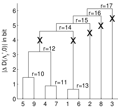
A detailed description of the entire procedure can be found in Algorithm 2 where labels the clusters in ascending order and (a two-dimensional array) is used to store a history of the mergings performed during different stages of the clustering procedure. In Figure 3(a) the merging process is illustrated for an exemplary scenario. A graphical representation of the mergings performed during different stages of the optimization, the so-called dendrogram [12], is shown in Figure 3(b).

 (a)
(b)
(a)
(b)
21
21
21
21
21
21
21
21
21
21
21
21
21
21
21
21
21
21
21
21
21
Using the dendrogram derived before, the source clusters with a maximum cluster size of can be constructed. We start at the root of the dendrogram, which is basically a tree, and descend along its branches to lower hierarchical levels. While moving from one level to the next lower one, the dendrogram branches into two subtrees. The number of leafs, i.e. the number of sources connected to each subtree are counted and if the number of leafs of one (or both) subtree(s) is smaller or equal to , we cut the corresponding subtree out of the dendrogram. This pruning process is repeated until all leafs are removed from the dendrogram. When the pruning is finished, the subtrees are labeled by the successively increased index . The source clusters , , can then be determined from the subtrees by assigning the variables (associated with each of the subtree’s leafs) to the corresponding cluster. The overall KLD between the original PDF and the approximated PDF can then be calculated based on the resulting clusters
| (17) |
where is defined analog to (12). In Figure 3(b) the pruning process is illustrated for the previous example.
Because of the hierarchical merging concept based on local decisions, the proposed clustering algorithm is in general sub-optimal. However, the hierarchical approach has the advantage that the resulting dendrogram can be used elegantly to construct clusters with a bounded number of source variables .44 4 With partitional clustering methods, see e.g. [12], this would be an arguably difficult task.
In Appendix G it is shown that the computational complexity of source-optimized clustering (evaluated in a very pessimistic fashion) is of which makes the overall procedure feasible for medium to large values of . Furthermore, it is easy to show that the number of clusters with a maximum cluster size of is bounded according to which shall be required in the next section.
IV-C Source-Optimized Factorization
In the last section we have shown how to construct KLD optimized clusters fitting our purposes. The second step towards our goal of obtaining a source factorization is to transduce the derived clusters into a symmetric CCRE of the form matching the conditions in (11). This can be achieved by linking the clusters , , successively together.
The basic principle of the linking procedure is as follows: After choosing a specific cluster as starting point for the procedure, select one of the unconnected clusters (i.e. a cluster which is not yet considered in the source factorization) and link it with the already connected clusters (i.e. incorporate it into the source factorization). Assuming that cluster was chosen as the starting point for the optimization, we can define a set of linked clusters and a set of unconnected clusters . At each step of the procedure a cluster and a cluster are selected. The index is added to the set of linked clusters, i.e. , and removed from the set unconnected clusters, i.e. . This is repeated until all clusters are linked, i.e. .
More specifically, two clusters are linked by choosing a set of variables and a set of variables . These sets will form the basis of the factor introduced into the source factorization. Since the complexity of scalable decoding is highly dependent on the number of variables within the single factors of the underlying source factorization (see Appendix F or [2] for details), we introduce the design parameters and such that and for all .
The source factorization starts with a single factor containing the variables of the initially chosen cluster , i.e. . While establishing a link between the two clusters and , the factors and are added to the source factorization where . As the clusters are linked, a source factorization is constructed step-by-step where the running index is used to index the added clusters. The resulting source factorization can then be written as
| (18) |
where and all factors with for are discarded. Notice that, when constructed according to the aforementioned linking procedure, there exists a one-to-one correspondence between the running index and the cluster indices . Moreover, it can easily be shown that (18) fullfills the criteria of CCREs by verifying the conditions in (11).
After discussing how source factorizations fitting our purposes can be constructed, we are ready to show how to choose the subsets and and in which order the clusters should be linked such that the overall KLD defined analog to (12) is minimized.
It is easy to show that the KLD of the source factorization given in (18) can be expressed as
| (19) | |||||
The KLD benefit imposed by the factors (c) in (18) can be written
| (20) | |||||
since the covariance matrices and are symmetric and positive-semidefinite and, thus, the determinants and are non-negative. Similarly, the KLD benefit imposed by the factors (b) in (18) can be expressed as
| (21) |
Considering the KLD benefit in (20) and (21), we notice that in (20) already was considered during the cluster optimization in Section IV . Thus, we are able to define the KLD benefit of establishing a link based on the sets and as
| (22) |
Using (17), the KLD of the source factorization in (18) can be written as
| (23) |
decoupling the link optimization from the cluster optimization.
If an already linked cluster is to be connected to a cluster in a KLD optimal way, then the sets and have to be chosen such that the KLD benefit according to (22) is maximized in magnitude. The set of all possible subsets with is denoted as and the set of all possible subsets with is denoted as . and are therefore defined as
| (24) |
and we define link cost as
| (25) |
Notice that generally .
To determine how the clusters are to be linked (i.e. which clusters are to be linked and in which direction), a graph can be constructed representing the KLD optimal links between the clusters. The vertices of the graph are obtained by contracting each cluster , with , to a single vertex and defining the set of vertices as
The set of all possible directed edges between the vertices and , , is defined as
where the cost of each edge in terms of KLD benefit is given by (25). A fully connected graph is thus obtained. Provided that the clusters are considered fixed, the overall KLD of the source factorization (18) can be optimized solely by optimizing the cluster links, please refer to (23), which are in turn represented by the directed edges in . The optimization problem therefore reduces to the Minimum (cost) Directed Spanning Tree (MDST) problem for which first algorithms were found by Chu and Liu [6] as well as by Edmonds [9] to be generalized later by Georgiadis [11]. After applying one of these algorithms to the fully connected graph , the MDST with and its root vertex (i.e. the vertex which only has outgoing edges) can be found. The source factorization (18) can then be constructed by moving along the edges of the obtained tree (possibly inspired by a Depth-First Search, see e.g. [1, p. 484]) and linking the clusters corresponding to the visited vertices together. More specifically, the root vertex of corresponds to the factor denoted as (a) in (18), the visited edges correspond to the factors denoted as (b) and the visited vertices correspond to the factors denoted as (c). Notice that this tree-based linking approach also conforms with the aforementioned linking procedure, which requires that links result only from already connected clusters, and thus guarantees a valid CCRE.
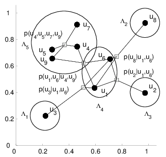
Considering the previous example with clusters , , , , and , we get the MDST with , root and . Figure 4 shows the corresponding source factorization.
Appendix H discusses the complexity of the source-optimized linking procedure and shows that the computational complexity grows exponentially with assuming that , which makes the overall procedure feasible for small cluster sizes . Notice that in the last section it was shown that allowing us to represent the complexity only based on the system parameters and . It is easy to see that, because the linking procedure basically constructs a tree between the clusters, the number of factors in the factorization (10) can be bounded according to . This also means that the number of factors with a maximum size of is at most , as used in Section IV-A to analyze the complexity of the scalable decoder.
V Results and Discussion
To underline the effectiveness and efficiency of our low-complexity coding and clustering strategies, we present numerical performance results for two scenarios with randomly placed sensors and two instances of the so-called CEO Problem [26].
V-A Randomly Placed Sensors
We consider a unit square with uniformly distributed sensors. The sensor measurements are Gaussian distributed according to . As outlined in Section II-A, we assume that sensor measurements are distributed according to a multivariate Gaussian distribution , where the correlation between a pair of sensors and decreases exponentially with the distance between them, such that . Since the performance of our techniques depend on the correlations between the sensors, we consider two different scenarios, one with (strongly correlated sensor measurements) and one with (weakly correlated measurements). All scalar quantizers at the encoders are Lloyd-Max optimized to minimize the MSE in the sensor readings using identical resolution for quantization and identical rates for data transmission, i.e. and for all , , where was chosen. The clusters indexed by are derived as described in Section IV-B where a maximum cluster size of was chosen, see Figure 5.
The index assignments are then designed successively for all clusters with and by employing the IR algorithm described in Section III with . Since it is not possible to construct index assignments for single-element clusters, we chose in this case a scalar quantizer (Lloyd-Max optimized as before) with decreased resolution and no index assignments such that is still guaranteed for all encoders . The source factorization used for decoding is constructed as described in Section IV-C assuming that , see Figure 5. The decoder is based on the sum-product algorithm as described in [2] where the required PMFs were obtained by Monte Carlo simulation using Lloyd-Max optimized quantizers with resolution for all . To evaluate the performance of the coding strategies, we measure the output signal-to-noise ratio (SNR) given by
averaged over a source samples.
| [bit] | 1 | 2 | 3 | 4 | 1 | 2 | 3 | 4 |
|---|---|---|---|---|---|---|---|---|
| [dB] | 4.44 | 9.46 | 14.61 | 20.32 | 4.45 | 9.32 | 14.65 | 20.27 |
| [dB] | 11.07 | 14.86 | 18.29 | N.A. | 7.54 | 11.72 | 16.21 | N.A. |
The simulation results of our system are depicted in Table I for strongly and weakly correlated sources. In both scenarios, we consider the performance achieved when using scalar quantization alone at the encoder, i.e. where the performance is mainly governed by the properties of the decoder (Dec), and the performance achieved when scalar quantization with a subsequent index-reuse (IR) is used for encoding. Table entries labeled as N.A. (not available) indicate that those instances could not be considered here due to their high computational demand.55 5 This instance would require a high-rate quantizer with a resolution larger than . Notice that only the index assignments yielding best possible performance were chosen for the experiments (e.g. a rate of [bits/sample] may be obtained from quantizers of resolution ).
Our simulation results reveal that simple index assignment techniques applied to local clusters can achieve significant performance gains using our coding approach, especially for low data rates and strongly correlated sources.
V-B The CEO Problem
In the following, we show the applicability of our techniques to another relevant sensor network model: the quadratic Gaussian CEO Problem [3]. Let be the output of a continuous-valued Gaussian source . For all , , let denote noisy observations of which are corrupted by additive noise, i.e. . The noise samples are generated by Gaussian noise processes statistically independent over . The observations are encoded and transmitted by independently operating encoders indexed by . The main task of the CEO is to estimate based on the data obtained from the encoders. In [15] we derived the optimal decoding rule exploiting the special properties of this problem setup and studied a feasible decoder using a source approximation based on the factorization
which can be easily represented by a factor graph [14]. In the following, we consider a scenario of encoders. The source process is Gaussian distributed with mean and variance . The noise processes are Gaussian distributed with mean and variance for all where was chosen depending on the considered scenario. All scalar quantizers at the encoders are Lloyd-Max optimized to minimize the MSE in the sensor readings using identical resolution for quantization and identical rates for data transmission, i.e. and for all where was chosen. We use the scalable decoder as described in Section II where the required PMFs were determined using Monte Carlo simulation with resolution for the source and for the observations for all . Notice that in case of our highly symmetric scenario, with , and , the probabilities can be considered identical for all . Therefore, the index assignments need to be designed only once for a single, arbitrarily chosen cluster with where was chosen. After employing the IR algorithm described in Section III with and , the resulting index assignments can be assigned repeatedly to all clusters within the system. To evaluate the performance of our coding strategies, we measure the output SNR for given by
versus the (symmetric) encoder transmission rate averaged over source samples and compare it with the (sum) rate-distortion function, offered by [5], which presents an upper bound found to be tight for noise processes with identical variance. In Table II we present some results to underline the effectiveness of our approach. The performance of the system without index assignments (Dec) and the performance obtained by using index-reuse (IR) is compared to the theoretically possible value as given by the (sum) rate-distortion function (R/D) according to [5]. Table entries labeled as N.A. (not available) indicate that those instance could not be considered here due to their high computational demand.66 6 This instance would require a high-rate quantizer with a resolution larger than . Table entries labeled as N.B. (no benefit) indicate that in this case index-reuse does not outperform standard quantization. Notice that only the index assignments yielding the best possible performance were chosen for the experiments.
| =1, =0.1 | =1, =0.5 | |||||||
|---|---|---|---|---|---|---|---|---|
| [bit] | 1 | 2 | 3 | 4 | 1 | 2 | 3 | 4 |
| [dB] | 28.66 | 29.70 | 29.93 | 29.99 | 21.72 | 22.74 | 22.96 | 23.01 |
| [dB] | 9.67 | 19.37 | 26.21 | 28.48 | 15.25 | 20.84 | 22.49 | 22.74 |
| [dB] | 22.71 | 26.70 | 28.21 | N.A. | 18.76 | 21.56 | N.B. | N.A. |
The numerical results reveal that our index-reuse approach leads in many cases to significant performance improvements over standard quantization. It might happen, however, that our index assignments are not able to outperform scalar quantization. Whether or not this is true depends on several factors: (a) the quantizer resolution , (b) the number of output bits and (c) the correlation properties of the sources determined by and . In cases where the sources are weakly correlated, e.g. for large values of , it becomes harder (or even impossible) to find index assignments that offer good rate/distortion trade-offs. In particular this might be true in our case due to the simplicity of the considered coding concept and the sub-optimality of the proposed index-reuse algorithm whose performance is highly dependent on the choice of and .
VI Concluding Remarks
We presented a scalable solution for distributed source coding in large-scale sensor networks. Our methods rely on the combination of a simple encoding stage (a scalar quantizer and an index assignment stage) and a source-optimized clustering algorithm. Despite the simplicity of the proposed techniques, our results show significant performance gains in comparison with standard scalar quantization. It is worth mentioning that the same ideas can be used together with other distributed source coding schemes, e.g. those based on syndromes [19], on Diophantine index assignments [16] or even on random index assignments. As part of our ongoing work we are considering the case in which the covariance matrix of the sensor observations is not known beforehand. Thus, each sensor must decide on-the-fly which code to use and inform the decoder. Finding distributed clustering and coding algorithms for this problem remains a challenging task.
Appendix A Optimal Decoding Rule
In this section, we want to derive a simple expression for the optimal decoding rule.
Let be the index identifying the source for which the estimate has to be calculated. Let be a set of indices identifying the encoders whose codewords, collected in the vector , are available for the calculation.
Specifically, we want to show that . We start by using the definition of the conditional expectation and apply the Bayes rule such that
| (26) |
Furthermore, we can state that
Since the index is constant for all that fall into the quantizer region such that , the integral in (26) can be splitted into separate parts and we obtain
| (27) |
We observe that and that
| (28) |
where the equality (a) holds since is either zero or unity depending on the fact if or, identically, if falls into the quantizer region such that . Therefore, we can state that
| (29) |
Using these results together with (27), the desired equality can be established easily.
Appendix B Efficient Marginalization and its Complexity
In this section, we want to characterize the complexity of the marginalization operation required at several points of this work, e.g. consider the calculation of the optimal estimate in (3) where the marginalization in (4) has to be performed using the argument in (5).
For a general treatment of the problem, we shall employ the same definitions as provided in Appendix A. Let furthermore be a set of indices identifying the sources whose discrete representations, collected in the vector , are involved within the calculation. Specifically, we shall consider the calculation of out of through the following marginalization
| (30) |
with and
| (31) |
where equality (a) obviously holds for , since in this case , and also for , since in this case does not provide any information about due to the fact that is known and for all such that .
In the most straightforward implementation of the marginalization in (30), the summation over has to be performed over all possible realizations of with where the actual value of can be calculated using the product representation in (31). It is worth pointing out that in (31) can become either zero or unity depending on the current configuration of the transition probabilities for all . This can be used to restrict the number of index tuples that have to be considered throughout the marginalization in (30), as shown in the following.
For brevity, we shall restrict ourselves to the case where , i.e. where .77 7 The results for the case can be derived accordingly. Let be the set of index tuples that are mapped onto .88 8 It is worth pointing out that can be constructed easily since the mapping functions are assumed to be known for all . Then, the marginalization in (30) can be expressed as follows:
| (32) | |||||
Notice that the marginalization according to (32) has to be performed, if it has to be performed at all, only over the members of the set . Since the cardinality of this set is much smaller than the cardinality of in (30) the complexity of the marginalization can be reduced considerably.
For a more detailed discussion of the complexity, the cardinality of the set shall be characterized in the following. Notice that denotes the set of indices that are mapped onto the codeword . The following result is usefull
Lemma B.1
For any surjective mapping function and any , .
Proof:
Since is a function each is mapped to exactly one . From this we conclude that (a) there are no that are mapped to more than one (mutual exclusivity) and (b) each is mapped to some . Since is a surjective function there exists an for any such that and we conclude that (c) for all . From (a) and (b) we obtain that which can be solved for an arbitrarily chosen , e.g. , and we obtain . Because of (c) we know that is maximal if for all and we obtain that for any establishing the claim. ∎Using this result, the complexity of the marginalization in (30) can be characterized. For the sake of a simple discussion, we assume that for all and that for all . Using Lemma B.1 and after defining the system specific parameter , we are able to conclude that in our case for any . We furthermore assume that the elementary operations (like additions, multiplications, comparisons, look-ups, etc.) are of constant complexity, i.e. of . Specifically, we assume that can be determined with a complexity of , e.g. that it can be approximated, simulated, etc. with constant complexity or that it can be looked-up.
In the following, we consider the newly derived expression for the marginalization (32). In the case where holds, it is easy to see that, in the worst-case, instances of are required throughout the calculation and that around additions have to be performed. Thus, around elementary operations have to be performed corresponding to a computational complexity of . In the case where does not hold, the result of the marginalization becomes zero, without any further calculations, and the computational complexity derives to be of for testing the case alone.
Appendix C Complexity of Optimal Decoding
In this section, which uses the same definitions as the previous appendices, we discuss the complexity of optimal decoding as required e.g. in (3). Specifically, we want to consider the calculation
| (33) |
We observe that the calculation in (33) requires that and have to be determined, multiplied and summed-up for all possible realizations of where can be derived from using the efficient marginalization described in Appendix B.
In order to use the results derived in Appendix B, we restrict ourselves to the case where , i.e. where .99 9 The results for the case can be derived accordingly. For a simplified complexity analysis, we furthermore assume that , and for all where . Elementary operations (like additions, multiplications, comparisons, look-ups, etc.) are assumed to be of constant complexity, i.e. of . Specifically, we assume that and can be determined with a complexity of , e.g. that they can be approximated, simulated, etc. with constant complexity or that they can be looked-up.
Using the results of Appendix B, we are able to state that the computational complexity for deriving , as required in (33), is of or of depending on the fact whether is mapped onto or not. In order to determine the overall complexity, we notice that the summation in (33) has to be performed over all . Therefore, we can employ Lemma B.1 in Appendix B to determine how often it will be true (at most) that and, thus, how often (at most) the calculation of in (4) has to be performed. We conclude that this calculation has to be performed (at most) times. The test if is true, the look-up of as well as the multiplication in (33) can be neglected compared to the complexity of calculating in total times. Therefore, we are able to conclude that calculating one estimate has a computational complexity of .
Appendix D Distortion Calculation
In this section, which again uses the same definitions as the previous appendices, we shall show that the overall distortion associated with each source can be described by the sum
| (34) |
where is the distortion caused by the quantization stage and is the distortion caused by the index assignment stage.
To do so, we start with the definition of the expectation value and obtain
where the equality (a) holds due to the fact that the index assignments are surjective functions for all and, thus, the summation over all covers the same observation space as the summation over all . Based on this observation, equation (34) can easily be established by showing that
| (35) |
The definition of the conditional expectation allows us to rewrite
| (36) | |||||
where the definition of the conditional expectation is used in (a) together with the fact that for all , equality (b) is valid since is known if is known and, thus, and equality (c) holds due to (29). Assuming that
| (37) |
i.e. that the reconstruction value of the quantizer is the centroid of the quantization region, it is possible to show that the required integration can be split into two parts1010 10 This can be achieved by substituting , where , such that can be expressed as which derives to . such that
| (38) |
where . Plugging (38) into (36), we obtain
| (39) | |||||
directly establishing (35) and, thus, the desired result in (34).
Appendix E Complexity of the Index-Reuse Optimization
The computational complexity of the index-reuse algorithm presented in Algorithm 1 can be bounded by evaluating how often, in the worst-case, the operations within the innermost of the nested loops have to be performed.
The outermost loop is executed for each of the mergings that have to be performed to obtain mappings with output codewords from the initial mapping with output codewords. The second loop is executed for all considered encoders , i.e. in total times. Finally, the innermost loop runs through all possibilities of choosing out of codewords for the merging, i.e. we have possibilities. In the worst-case, i.e. in the initial case where , we obtain possibilities. Thus, the operations within the innermost loop have to be performed times in the worst-case.
Now, to determine the overall complexity of the algorithm the complexities of the merging operation , the complexity of the distortion calculation and the test if have to be determined. Assuming that the merging and the test can be performed with a constant computational complexity of , it remains to determine the complexity of calculating given the current set of mapping functions . This calculation requires the calculation of according to (8) which, in turn, requires the calculation of the estimate according to (3) for all possible realizations of .1111 11 There are more efficient ways to calculate based on intermediate results. However, due to lack of space, the discussion is neglected here. Assuming that , i.e. that , the result of Appendix C directly applies here and we can state that calculating one estimate has a computational complexity of .1212 12 The results for the case where can be derived accordingly. Thus, in the most straightforward implementation, the computational complexity of calculating according to (8) is of .
Based on the presented results and after substituting by , as derived in Appendix B for surjective mapping functions, we are able to conclude that the overall computational complexity of the index-reuse algorithm is of showing an exponential growth with .
Appendix F Efficient Sub-Optimal Decoding and its Complexity
In this section, which uses the same definitions as the previous appendices, we shall elaborate on how a source factorization based on CCREs according to (10) and (11) can be used for efficient decoding. This shall be achieved by assuming that the factorization (10) also holds for the discrete case1313 13 This assumption is plausible since forms a Markov chain for . such that
| (40) |
a fact, which can be exploited for scalable decoding as shown in [2] for a similar system setup. Since the decoder design considered in this work follows the same principles, we shall focus on the differences resulting from system specific properties.
In Section II we have shown that the calculation of the optimal estimate according to (3) for requires the calculation of the probabilities
| (41) |
where the equality (a) is due to the result derived in Appendix B. Replacing by its approximation as given by the factorization in (40), we obtain the following approximation
| (42) |
which can be calculated efficiently for all and for all by running the sum-product algorithm on the factor graph representation of the factorization in (40). For a general treatment of factor graphs and the sum-product algorithm please refer to [14] or to [2] where a similar system setup is discussed.
In order to provide the fundamentals, we include a brief review here. A factor graph is a bipartite graph that consists of variable and function nodes and expresses how a (global) function factors into (local) functions. The variable nodes represent the arguments of the functions and the function nodes the (local) functions itself. The sum-product algorithm allows us to perform the (global) marginalization in (42) based on (local) marginalizations of the following type
| (43) |
which are performed in a structured way for all and . Following the intuition in [14], the results of the marginalizations in (43) for can be seen as messages represented a vector that are sent from the function node to the variable node for further processing. Similarly, the inputs of the marginalizations in (43) can also be seen as messages that were received at the function node originating from some variable nodes . Those messages represent the product
| (44) |
for and, thus, . Using this abstraction, the techniques described in [14] can be directly applied here giving rise to an efficient calculation of (42).1414 14 It is worth pointing out that the expression in (43) is optimized to minimize the marginalization complexity by using knowledge about the received codewords. This in turn means that in this particular setup the function nodes have to be initialized and not the variable nodes as in conventional implementations. Specifically, the function nodes are initialized by defining the set using knowledge of for and the variable nodes are initialized with trivial messages. In particular this is achieved by running an appropriate message passing algorithm1515 15 For factor graphs without cycles the efficient forward-backward algorithm can be employed, see [14]. along the factor graph representation of (40) and depending on the fact if the message passing procedure terminates or not, i.e. if the factor graph is cycle-free or not,1616 16 Using the result in [2] this can be ensured if for . the exact or an approximated value of is obtained simultaneously for all and .
Since the presented decoding scheme is based on message passing, its overall complexity can be analyzed by considering all messages that are created during the decoding process and jointly evaluating their complexity. We notice that the calculation of the messages at each function node according to (43) requires a marginalization of the same type as discussed in Appendix B. Assuming that furthermore and for and that the complexity of elementary operations are the same as stated in Appendix B, the derived results directly apply here and we are able to conclude that the messages at the function nodes can be created with a computational complexity of . Considering the messages created at the variable nodes according to (44), it is easy to see that the messages can be derived with a computational complexity of . We notice that the complexity of calculating the messages at the function nodes is higher than at the variable nodes since generally for all (but maybe one) , i.e. the complexity of calculating the messages at the variable nodes can be neglected here. In order to provide an expression for the complexity, we have to distinguish between two cases.
In the case where the factor graph is cycle-free, the efficient forward-backward algorithm, see [14], can be used for message passing and only one message (in each direction) needs to be passed along each edge within the graph. Assuming that for all , the calculation in (43) has to be performed at most times leading to a computational complexity of . In the case where the graph has cycles, the message passing has to be performed in an iterative way for an reasonable amount of iterations , see [14], and we obtain a computational complexity of .
Appendix G Complexity of Source-Optimized Clustering
The complexity of source-optimized clustering used in Section IV-B shall be discussed next.1717 17 The main goal at this point is to show that source-optimized clustering is of polynominal complexity (considering the number of sources ) and not to find an exact expression for the complexity of Algorithm 2. This would exceed the scope of this work. In [12] it is shown that hierarchical clustering, upon which the presented procedure is based, has a computational complexity of . However, these results do not directly hold for source-optimized clustering since for each step of the procedure, i.e. for each merging performed, the differential KLD benefit according to (16) has to be calculated. Looking at (16) in more detail, we observe that merging cluster and requires the calculation of the KLD benefit according to (14) which, in turn, requires the calculation of the determinant for the corresponding covariance matrix . Using the general definition of determinants, it is easy to see that it can be calculated using Gaussian elimination. Assuming that the matrix, whose determinant has to be derived, is of size , then the complexity of the Gaussian elimination and, thus, also of calculating the determinant is of , see e.g. [25].1818 18 There are more efficient ways to calculate the determinant of a matrix, see e.g. [25], but it is sufficient for our purposes to assume that the Gaussian elimination is used. Since is always smaller or equal to , the matrix is (at most) of size and, thus, the calculation of is of . Assuming that the complexity of performing one merging step within the classical hierarchical clustering algorithm is of , i.e. the minimum possible, then the number of mergings to be performed can be bounded by . For the source-optimized clustering procedure this means that its computational complexity is of .
Appendix H Complexity of Source-Optimized Linking
This section addresses the complexity of constructing the source-optimized factorization presented in Section IV-C. Using the result in [17], we are able to conclude that the directed spanning tree algorithm, upon which the presented procedure is based on, can be implemented with a complexity of . However, beside this, also the complexity of preprocessing the data required to initialize the directed spanning tree algorithm has to be considered. In particular this means that the link costs have to be determined before the directed spanning tree algorithm can be employed. In total there are link costs representing the KLD benefit associated with establishing a link between cluster , , and , , that have to be calculated according to (25). In order to calculate this link cost all possible combinations of and have to be evaluated as stated in (24). It is easy to see that the number of such combinations is given by the product between and where and . For simplicity, we assume in the following that and that for .1919 19 For other configurations the following results can be derived accordingly. After simple mathematical manipulation we are able to conclude that there are at most such combinations. It remains to derive the complexity of calculating the argument in (24), i.e. the complexity of calculating according to (22), which is clearly determined by the complexity of calculating according to (14). Using the same arguments as in Appendix G, we can state that the complexity of calculating the determinant in (14) is of , i.e. it is of using the same assumptions as before. Putting everything together, we are able to conclude that the calculation of all link cost is of . The computational complexity of the overall source-optimized linking procedure is then given by the sum of the derived complexities, i.e. of the directed spanning tree algorithm and the link cost calculation. Since the complexity of the algorithm can be neglected here, we conclude that the complexity of source-optimized linking is of which is only feasible for small values of .
References
- [1] Alfred V. Aho and Jeffrey D. Ullman. Foundations of Computer Science, C Edition. W. H. Freeman & Co., New York, NY, USA, 1997.
- [2] J. Barros and M. Tuechler. Scalable decoding on factor trees: A practical solution for sensor networks. IEEE Transactions on Communications, 54:284–294, 02 2006.
- [3] T. Berger, Z. Zhang, and H. Viswanathan. The CEO problem. IEEE Trans. Inform. Theory, 42:887–902, 1996.
- [4] Jean Cardinal and Gilles Van Assche. Joint entropy-constrained multiterminal quantization. In Proceedings of the International Symposium on Information Theory, Lausanne, Switzerland, 2002.
- [5] Jun Chen, Xin Zhang, Toby Berger, and Stephen B. Wicker. An upper bound on the sum-rate distortion function and its corresponding rate allocation schemes for the CEO problem. Special Issue of JSAC, On Fundamental Performance of Wireless Sensor Networks, May 2004.
- [6] Y. J. Chu and T. H. Liu. On the shortest arborescence of a directed graph. Science Sinica, 14:1396–1400, 1965.
- [7] T. M. Cover and J. Thomas. Elements of Information Theory. John Wiley and Sons, Inc., 1991.
- [8] C. R. Dietrich and G. N. Newsam. Fast and exact simulation of stationary Gaussian processes through circulant embedding of the covariance matrix. SIAM Journal on Scientific Computing, 18(4):1088–1107, 1997.
- [9] J. Edmonds. Optimum branchings. J. Research of the National Bureau of Standards, 71B:233–240, 1967.
- [10] T. J. Flynn and R. M. Gray. Encoding of correlated observations. IEEE Trans. Inform. Theory, IT-33(6):773–787, 1987.
- [11] Leonidas Georgiadis. Arborescence optimization problems solvable by Edmonds’ algorithm. Theor. Comput. Sci., 301(1-3):427–437, 2003.
- [12] A. K. Jain, M. N. Murty, and P. J. Flynn. Data clustering: a review. ACM Computing Surveys, 31(3):264–323, 1999.
- [13] N. Jayant and P. Noll. Digital Coding of Waveforms. Prentice Hall, 1984.
- [14] F. R. Kschischang, B. Frey, and H.-A. Loeliger. Factor graphs and the sum-product algorithm. IEEE Trans. Inform. Theory, 47(2):498–519, 2001.
- [15] G. Maierbacher and J. Barros. Low-complexity coding for the CEO problem with many encoders. In Twenty-sixt Syposium on Information Theory in the Benelux, Brussels, Belgium, 2005.
- [16] G. Maierbacher and J. Barros. Diophantine index assignments for distributed source coding. In Proceedings of the 2007 IEEE Information Theory Workshop (ITW 2007) - Frontiers in Coding, Lake Tahoe, California, USA, 2007.
- [17] Anna Nepomniaschaya. Efficient implementation of Edmonds’ algorithm for finding optimum branchings on associative parallel processors. In Proc. of the Eighth Intern. Conf. on Parallel and Distributed Systems (ICPADS’01), KyongJu City, Korea, 2001.
- [18] H. V. Poor. An Introduction to Signal Detection and Estimation. Springer-Verlag, 1994.
- [19] S. S. Pradhan and K. Ramchandran. Distributed source coding using syndromes (DISCUS): Design and construction. In Proc. IEEE Data Compression Conf. (DCC), Snowbird, UT, 1999.
- [20] S. Sandeep Pradhan and Kannan Ramchandran. Generalized coset codes for distributed binning. IEEE Trans. Inform. Theory, 51:3457–3474, 2005.
- [21] David Rebollo-Monedero, Rui Zhang, and Bernd Girod. Design of optimal quantizers for distributed source coding. In Proceedings of the Data Compression Conference (DCC’03), 2003.
- [22] A. Scaglione and S. D. Servetto. On the interdependence of routing and data compression in multi-hop sensor networks. In Proc. ACM MobiCom, Atlanta, GA, 2002.
- [23] S. D. Servetto. Lattice quantization with side information. In Proc. IEEE Data Compression Conf. (DCC), Snowbird, UT, 2000.
- [24] D. Slepian and J. K. Wolf. Noiseless coding of correlated information sources. IEEE Trans. Inform. Theory, IT-19(4):471–480, 1973.
- [25] Volker Strassen. Gaussian elimination is not optimal. Numer. Math., 13:354–356, 1969.
- [26] Harish Viswanathan and Toby Berger. The quadratic Gaussian CEO problem. IEEE Trans. Inform. Theory, 43:1549–1559, 1997.
- [27] J. Ward. Hierarchical grouping to optimize an objective function. Journal of the American Statistical Association, 58:236–244, 1963.
- [28] Z. Xiong, A. D. Liveris, and S. Cheng. Distributed source coding for sensor networks. IEEE Signal Processing Magazine, 09 2004.
- [29] R. Zamir, S. Shamai, and U. Erez. Nested linear/lattice codes for structured multiterminal binning. Information Theory, IEEE Transactions on, 48(6):1250–1276, 2002.