Robustness of Heisenberg-limited interferometry with balanced Fock states
Abstract
Interferometry with Heisenberg limited phase resolution may play an important role in the next generation of atomic clocks, gravitational wave detectors, and in quantum information science. For experimental implementations the robustness of the phase resolution is crucial since any experimental realization will be subject to imperfections. In this article we study the robustness of phase reconstruction with two number states as input subject to fluctuations in the state preparation. We find that the phase resolution is insensitive to fluctuations in the total number of particles and robust against noise in the number difference at the input. The phase resolution depends on the uncertainty in the number difference in a universal way that has a clear physical interpretation: Fundamental noise due to the Heisenberg limit and noise due to state preparation imperfection contribute essentially independently to the total uncertainty in the phase. For number difference uncertainties less than one the first noise source is dominant and the phase resolution is essentially Heisenberg limited. For number difference uncertainties greater than one the noise due to state preparation imperfection is dominant and the phase resolution deteriorates linearly with the number difference uncertainty.
pacs
42.50.Dv,06.20.-fdmeiser@jila.colorado.edu
1 Introduction
The precision with which phase shifts can be determined in an interferometer is ultimately limited by shot noise. The shot noise originates from the discreteness of the interfering particles 11 1 For conciseness we refer to the interfering objects as particles with the understanding that they could be realized as actual particles or field quanta such as photons.. For interferometry with independent particles, each particle interferes only with itself. For independent particles the precision is times better than the single particle precision, a result which follows from application of the central limit theorem. This scaling of the phase precision with the number of particles, is called the standard quantum limit.
In some applications an increase in the number of interfering particles is difficult or impractical. In these cases it is worth trying to make better use of the available resources. Interferometry with phase resolution better than the standard quantum limit is relevant for gravitational wave detectors [1, 2, 3]. The best atomic clocks employing [4, 5], trapped ions [6, 7], and earth-alkaline atoms such as in optical lattices [8, 9, 10, 11, 12] are also operating very close to the standard quantum limit. In the next generation of clocks the precision could be further increased by using interferometry with resolution better than the standard-quantum-limit.
Phase resolution better than the standard quantum limit can be achieved with entangled many particle states. A variety of such input states have been proposed. For interferometry with photons, squeezed states of light have been suggested. Bollinger and Wineland have proposed spin squeezed states for ions and other massive particles [13]. Maximally entangled states have been proposed theoretically [14, 15] and their improved phase resolution has been demonstrated experimentally [16]. Holland and Burnett have suggested to use Fock states in each of the input ports and they have shown that these states yield Heisenberg limited phase resolution [17]. States with improved phase resolution have been systematically studied in [18, 19, 20, 21, 22].
For linear interferometers the resolution achievable with particles is fundamentally limited to a scaling , called the Heisenberg limit.
So far, most studies of interferometry with resolution better than the standard quantum limit have concentrated on ideal realizations in which the initial state can be realized with perfect fidelity, no dephasing or decoherence happens during the evolution through the interferometer, and the final state is detected with ideal detectors. For the maximally entangled Schrödinger cat state, the effect of dephasing during the evolution through the interferometer has been studied by Huelga et al[23]. The effect of decorrelation on the phase resolution for interferometry with balanced Fock states has been studied by Kim et al[24] and recently Dorner et al[25] have constructed generalizations of maximally entangled states that are more robust against photon loss inside the interferometer.
The goal of this article is to study the robustness of the dual Fock state against imperfections in the creation of the initial state. We find that this state is insensitive to fluctuations in the total number of particles fed into the interferometer. The phase resolution is robust against fluctuations in the number difference. If the fluctuations in the number difference are of order one, the phase resolution is still essentially Heisenberg limited. For increasing imbalance uncertainty, the phase resolution degrades linearly and becomes standard quantum limited as the imbalance uncertainty approaches the partition noise. These findings add a whole class of states to the arsenal of states that are candidates for phase resolution better than the standard quantum limit. This class of states can be thought of as the incoherent cousin of the conventional squeezed states. The states are incoherent mixtures of number difference states with a probability distribution that is narrower than the partition noise.
2 Model
For the remainder of this article we consider the elementary Mach-Zehnder interferometer depicted in figure 1. Particles prepared in state pass through a beam splitter. The component passing through one of the arms experiences a phase shift relative to the other arm. The two modes are recombined at a second beam splitter and detectors measure the numbers of particles coming out in ports one and two.

We describe the particles passing through the interferometer as effective two level systems with the two states corresponding to the two arms of the interferometer. Mathematically we describe these two level systems using the angular momentum formalism. This formalism as it applies to interferometry has been described in detail in several articles, see for instance [21, 24, 26]. In brief, each particle is identified with a fictitious spin-1/2 system with spin up and down corresponding to the particle being in port one and two, respectively. A collection of particles is then described by combining the spins into a total angular momentum.
The -component of the total angular momentum describes the number imbalance between the ports of the interferometer and the square of the length of the angular momentum vector is related to the total number of interfering particles. We choose the and eigenstates with
and
and as basis states. The perfectly balanced Fock state suggested by Holland and Burnett is the state 22 2 For simplicity we restrict ourselves to even total numbers of particles. The case of odd numbers of particles is qualitatively identical.. The interferometer transformation that relates the output state to the input state is
From here on we specialize to the case of an interferometer with relative phase shift . For the balanced input states that we consider below this choice of working point corresponds to the null fringe were equal numbers of particles are detected in both output ports of the interferometer.
2.1 State preparation
In an ideal experiment it would be possible to deterministically create the state with fixed . However, for systems with large numbers of particles, where the precision gain would be most dramatic, this perfect situation cannot be achieved in general. In practice, states are created stochastically with a probability distribution . Typically it is impossible to determine which and were realized due to finite detector sensitivity. This means that one has to reconstruct the phase based on incomplete knowledge of the initial state.
It has been shown by Uys and Meystre [21] that the phase resolution for states depends very little on as long as . 33 3 In fact, these authors have shown that the phase resolution is nearly Heisenberg limited almost all the way to . We can therefore assume, without loss of generality, that the mean of the distribution is centered at in accordance with the original proposal of Holland and Burnett [17]. For the working point this is also the most interesting case from an experimental perspective, where it is advantageous to detect approximately equal numbers of particles in both detectors due to finite detector efficiency. Modeling the distribution as a Gaussian distribution in and we can characterize the state preparation by three parameters: the average total angular momentum and the standard deviations and of the distributions of the total angular momentum , , and of the number imbalance , . From now on we refer to as the state preparation imperfection or just imperfection for brevity. The initial state is then a statistical mixture,
| (1) |
2.2 Phase reconstruction: Bayesian inference and likelihood function
It is well known that reconstructing the phase shift from a measurement record is a non-trivial task if the input state of the interferometer is the balanced Fock state. For that state, the mean number imbalance is zero for all phase shifts and hence cannot be used as a signal. The variance varies sinusoidally with the phase, but the signal-to-noise ratio of that observable is of order one. Thus a large number of measurements are necessary in order to infer the phase shift. It can be shown that the same holds true for all higher moments of as well. In order to achieve that state’s potential phase resolution, one has to use a Bayesian reconstruction scheme instead [17]. This scheme has the additional advantage that it yields the full probability distribution of the phase conditioned on a measurement record instead of e.g. the first few moments. Furthermore, it immediately yields a prescription for how to find the phase in an actual experiment.
The basic idea of Bayesian inference is to update the probability distribution of the phase according to
| (2) |
with a normalization constant. Note that we use the symbol to denote different normalization constants throughout this article whose precise value is irrelevant. The prior phase distribution contains all the knowledge available about the phase before the first measurement. To provide an unbiased analysis of the phase measurement we assume that nothing is known about the phase initially except that it lies in the interval . 44 4 This choice of the prior phase distribution makes this phase inference method essentially a maximum likelihood estimation. This latter restriction removes the irrelevant phase ambiguity where phases that differ from each other by an integer multiple of cannot be distinguished. The prior phase distribution is then
| (3) |
is the conditional probability for a number difference to occur given that the phase shift was . The denominator normalizes the probability distribution .
Equation (2) can be iterated: After a measurement of the number difference the knowledge about the phase is . The phase distribution after a second measurement is then obtained from equation (2) by using as the prior. For a measurement record one finds the phase distribution
| (4) |
The sharpness of this distribution after a certain number of measurements is a figure of merit of the phase resolution obtainable with a given input state.
In the limit of a large number of measurements the various possible measurement outcomes occur times, where is the actual phase shift. The phase distribution then becomes
| (5) | |||||
| (6) |
with
| (7) |
The function is the asymptotic likelihood function of the phase. It fully characterizes the expected phase resolution in the limit of large .
3 Results
3.1 Conditional probabilities
From equation (2) it is clear that the conditional probabilities are of central importance for the phase resolution. The sharper the distribution is as a function of , the more one learns about the phase if the number difference is detected. However it is not sufficient for a state to have sharply peaked distributions in order to be useful for interferometry. Measurement outcomes with such sharp distributions also must be likely to occur. This latter requirement makes the phase resolution typically dependent on the working point of the interferometer, i.e. the precision depends on the phase that one wishes to measure.
The conditional probabilities are calculated by sending the initial state of equation (1) through the interferometer and projecting the final state on the subspace with a given ,
| (8) |
where is the projector on the subspace,
The conditional probabilities for a well defined initial and , , behave as
| (9) |
for phase shifts small enough so that the number differences near the poles of the Bloch sphere are unlikely. In this equation is the Bessel function of the first kind of order .
In Figure 2 we show the conditional probabilities for various initial states for an average of 20 particles, i.e. . As a consequence of the Bessel function like behavior, the conditional probability for perfect state preparation in figure 2(a) is sharply peaked at with a width of order . This sharp peak gives rise to Heisenberg limited phase resolution for the perfectly balanced Fock state. For larger phase shifts the conditional probabilities oscillate with frequency and with an envelope falling off as .
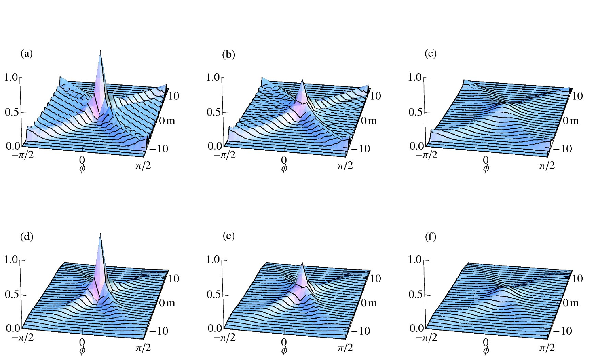
Figures 2(b,c) show that the width of the peak of the conditional probabilities increases with increasing state preparation imperfection . Qualitatively, it is clear that this increased width leads to a decreasing phase resolution. The width of the central peak can be estimated by the construction illustrated in figure 3(a). For phase shifts the maxima of the distribution follow the red lines given by . Mathematically, this follows from properties of the Bessel-functions which describe the conditional probabilities well for . Qualitatively, the scaling of with can be understood by noting that the number difference has to increase from zero to for a phase shift of . These lines translate the Gaussian distribution of with width into a Gaussian distribution of the phase with width
| (10) |
This Gaussian is compared with the exact probability distribution in figure 3(b). The central portion of that probability distribution is well described by the Gaussian. The wings of the conditional probability distributions can be found from the asymptotic behavior of the Bessel functions. Averaging several Bessel functions leads to the tails falling off as
| (11) |
This is also illustrated in figure 3(b). Note that in a phase reconstruction experiment the wings get more and more suppressed with increasing number of measurements and eventually the phase distribution is entirely determined by the approximately Gaussian central peak.


The figures 2(d-f) show the same conditional probabilities as in the panels (a-c) but with . As a consequence of the addition of Bessel functions that asymptotically oscillate with different frequencies the oscillations in the tails wash out for phase shifts in figure 2(d). Near the poles of the Bloch sphere the distributions look different compared to case with a sharp total number of particles, , because the total angular momentum now has a spread. Most importantly however, the central Gaussian peak is unaffected by the noise in . This is true for noise up to . As a consequence, the phase reconstruction is largely insensitive to this type of noise. Physically, this is because the measurement is based on detection of number differences in which the total number of particles cancels out. Only when the phase shift is so large that almost all particles exit the interferometer in one port does the total number of particles play a role. We have numerically confirmed this independence of the phase resolution of . That allows us to consider the limit from now on without loss of generality.
3.2 Simulation of phase reconstruction: Finite numbers of measurements
To illustrate one of the key new features of phase reconstruction with imperfect state preparation compared to the ideal case we simulate an actual phase reconstruction experiment. As in the numerical examples in the previous section we consider a total particle number of and the state preparation imperfection is .
To simulate the phase reconstruction we draw a sequence of measurement results at random with probabilities given by . Using the known conditional probabilities we then successively update the phase distribution by means of Bayes’ formula. The evolution of the phase distribution with successive measurements is not deterministic due to the stochastic process with which the measurement results are determined.
Two representative examples of such phase reconstruction simulations are shown in figure (4). The first example is reminiscent of phase reconstruction with perfect state preparation. The phase distribution is centered at the correct phase shift and the width of the distribution shrinks monotonically with increasing number of measurements.
The second example illustrates a complication that can happen with imperfect state preparation. In the fourth measurement of that sequence a number difference of is detected. For the state preparation imperfection this measurement outcome is relatively unlikely to occur for zero phase shift and the Bayesian updating wrongly attributes the measurement result to a non-zero phase shift. The phase distribution becomes wider and is peaked at non-zero phase shift. Thus this unfavorable measurement outcome reduces the phase resolution and, even worse, it leads to an inaccurate phase inference. Further measurements correct this measurement and in the limit of large numbers of measurements the phase inference is accurate.


General quantitative statements on how many measurements are necessary in order to rule out such inaccuracies for a certain level of state preparation imperfection are difficult to make. In practice it is probably easiest to simply run numerical simulations of the phase reconstruction in order to empirically decide how many measurements should be made.
3.3 Asymptotic phase resolution
Asymptotically, the phase resolution improves as , where is the number of measurements. A figure of merit that is independent of the number of measurements and characterizes the suitability of an input state for phase measurements is therefore
| (12) |
where is the standard deviation of the phase distribution after measurements. We can calculate through the variance of the phase distribution given in equation (6) with an that is large enough so that the scaling equation (12) holds. For the results that follow we have used . This asymptotic phase distribution is devoid of the statistical fluctuations encountered in the previous section for small numbers of measurements.

We have numerically calculated the asymptotic phase resolution as a function of for different values of . The results are shown in figure 5. In that figure we have rescaled the phase resolution by . Remarkably, the resolutions for different rescaled this way all collapse onto a single universal curve. For nearly perfect state preparation the resolution saturates at the Heisenberg limit,
| (13) |
For , increases linearly with .
The universal behavior of can be understood by treating the fundamental noise due to the Heisenberg limit and the noise due to the state preparation imperfection as two independent noise sources. The total noise is then obtained by adding these noise sources in quadrature. According to the construction explained in figure 3 the noise due to the state preparation imperfection is given by , where is a constant of order one. describes by how much is broadened compared to the Gaussian in figure 3(b) due to the admixture of results . Adding then the Heisenberg limit noise and the state preparation noise in quadrature we find
| (14) |
This scaling of the phase resolution with and state preparation imperfection is the central result of this article. We find excellent agreement between equation (14) and the numerically determined phase resolutions for , as illustrated by the purple line in figure 5.
3.4 Phase reconstruction with unknown
In a typical experiment one will not precisely know the initial number difference uncertainty . Especially in light of the numerical simulations for finite numbers of measurements presented in section 3.2 it is important to understand the dependence of the phase inference on the choice of an estimate for . In particular one needs to know under what circumstances the phase distribution is asymptotically accurate. Or, phrased differently, how should one estimate so that unfavorable measurement results like in figure 4(b) are eventually corrected by a large number of measurements.

This problem can be studied by looking at the likelihood function of equation (7) as a function of the estimate for the number difference uncertainty. Basically one pretends that the number difference fluctuations are and calculates the corresponding conditional probabilities using the initial state with imperfection . But in an actual experiment each measurement result occurs with probability where the true fluctuations may differ from our estimate . In the limit of a large number of measurements the phase distribution is then governed by the likelihood function
| (15) |
That function is shown in figure (6) for , , and . The figure illustrates two typical properties of . If the estimate of the fluctuations is too optimistic, i.e. if , the likelihood is peaked at a non-zero phase shift and it has a minimum at zero phase shift. For such estimates the phase distribution is asymptotically inaccurate. This is because for a too optimistic estimate of one observes non-zero number differences at the output too often to be brought about by a non-zero phase shift. One thus wrongly concludes that the phase shift was non-zero.
For conservative estimates on the other hand the likelihood function of the phase is peaked at zero but it is broadened compared to the likelihood function for perfect knowledge of the number fluctuations, . As expected, the best phase resolution is obtained for .
4 Conclusion
Interferometry with balanced Fock states is robust against imperfections in the state preparation. The phase resolution is insensitive to noise in the total number of particles. For number difference uncertainties smaller than one the phase resolution is essentially Heisenberg limited. For larger state preparation imperfections the phase resolution deteriorates linearly with the number difference uncertainty.
In future work we plan to study the robustness of interferometry with balanced Fock states against dephasing and decoherence inside the interferometer as well as the effect of non-ideal detectors.
References
References
- [1] E. Gustafson et al. LIGO T990080-00-D, 1999; http://www.ligo.caltech.edu/docs/T/T990080-00.pdf.
- [2] H. J. Kimble, Yuri Levin, Andrey B. Matsko, Kip S. Thorne, and Sergey P. Vyatchanin. Conversion of conventional gravitational-wave interferometers into quantum nondemolition interferometers by modifying their input and/or output optics. Phys. Rev. D, 65(2):022002, Dec 2001.
- [3] Kirk McKenzie, Daniel A. Shaddock, David E. McClelland, Ben C. Buchler, and Ping Koy Lam. Experimental demonstration of a squeezing-enhanced power-recycled Michelson interferometer for gravitational wave detection. Phys. Rev. Lett., 88(23):231102, May 2002.
- [4] G. Santarelli, Ph. Laurent, P. Lemonde, A. Clairon, A. G. Mann, S. Chang, A. N. Luiten, and C. Salomon. Quantum projection noise in an atomic fountain: A high stability cesium frequency standard. Phys. Rev. Lett., 82(23):4619–4622, Jun 1999.
- [5] F. Pereira Dos Santos, H. Marion, S. Bize, Y. Sortais, A. Clairon, and C. Salomon. Controlling the cold collision shift in high precision atomic interferometry. Phys. Rev. Lett., 89(23):233004, Nov 2002.
- [6] W. H. Oskay, S. A. Diddams, E. A. Donley, T. M. Fortier, T. P. Heavner, L. Hollberg, W. M. Itano, S. R. Jefferts, M. J. Delaney, K. Kim, F. Levi, T. E. Parker, and J. C. Bergquist. Single-atom optical clock with high accuracy. Phys. Rev. Lett., 97(2):020801, 2006.
- [7] T. Rosenband, D. B. Hume, P. O. Schmidt, C. W. Chou, A. Brusch, L. Lorini, W. H. Oskay, R. E. Drullinger, T. M. Fortier, J. E. Stalnaker, S. A. Diddams, W. C. Swann, N. R. Newbury, W. M. Itano, D. J. Wineland, and J. C. Bergquist. Frequency Ratio of Al+ and Hg+ Single-Ion Optical Clocks; Metrology at the 17th Decimal Place. Science, 319(5871):1808–1812, 2008.
- [8] M. Takamoto, F.-L. Hong, R. Higashi, and H. Katori. An optical lattice clock. Nature (London), 435:321, 2005.
- [9] Andrew D. Ludlow, Martin M. Boyd, Tanya Zelevinsky, Seth M. Foreman, Sebastian Blatt, Mark Notcutt, Tetsuya Ido, and Jun Ye. Systematic study of the 87Sr clock transition in an optical lattice. Phys. Rev. Lett., 96(3):033003, 2006.
- [10] R. Le Targat et al. . Phys. Rev. Lett., 97:130801, 2006.
- [11] M. M. Boyd et al. Phys. Rev. Lett., 98:083002, 2007.
- [12] A. D. Ludlow et al. Science, 319:1805, 2008.
- [13] D. J. Wineland, J. J. Bollinger, W. M. Itano, F. L. Moore, and D. J. Heinzen. Spin squeezing and reduced quantum noise in spectroscopy. Phys. Rev. A, 46(11):R6797–R6800, Dec 1992.
- [14] J. J . Bollinger, Wayne M. Itano, D. J. Wineland, and D. J. Heinzen. Optimal frequency measurements with maximally correlated states. Phys. Rev. A, 54(6):R4649–R4652, Dec 1996.
- [15] Vittorio Giovannetti, Seth Lloyd, and Lorenzo Maccone. Quantum-Enhanced Measurements: Beating the Standard Quantum Limit. Science, 306(5700):1330–1336, 2004.
- [16] V. Meyer, M. A. Rowe, D. Kielpinski, C. A. Sackett, W. M. Itano, C. Monroe, and D. J. Wineland. Experimental demonstration of entanglement-enhanced rotation angle estimation using trapped ions. Phys. Rev. Lett., 86(26):5870–5873, Jun 2001.
- [17] M. J. Holland and K. Burnett. Interferometric detection of optical phase shifts at the Heisenberg limit. Phys. Rev. Lett., 71(9):1355–1358, Aug 1993.
- [18] G. S. Summy and D. T. Pegg. Phase optimized quantum states of light. Opt. Comm., 77:75, 1990.
- [19] D. W. Berry and H. M. Wiseman. Optimal states and almost optimal adaptive measurements for quantum interferometry. Phys. Rev. Lett., 85(24):5098–5101, Dec 2000.
- [20] A. Luis and J. Peřina. Optimum phase-shift estimation and the quantum description of the phase difference. Phys. Rev. A, 54(5):4564–4570, Nov 1996.
- [21] H. Uys and P. Meystre. Quantum states for Heisenberg limited interferometry. Phys. Rev. A, 76:013904, 2007.
- [22] Y. P. Huang and M. G. Moore. Optimized double-well quantum interferometry with gaussian squeezed states. Phys. Rev. Lett., 100(25):250406, 2008.
- [23] S. F. Huelga, C. Macchiavello, T. Pellizzari, A. K. Ekert, M. B. Plenio, and J. I. Cirac. Improvement of frequency standards with quantum entanglement. Phys. Rev. Lett., 79(20):3865–3868, Nov 1997.
- [24] Taesoo Kim, Olivier Pfister, Murray J. Holland, Jaewoo Noh, and John L. Hall. Influence of decorrelation on Heisenberg-limited interferometry with quantum correlated photons. Phys. Rev. A, 57(5):4004–4013, May 1998.
- [25] U. Dorner, R. Demkowicz-Dobrzanski, B. J. Smith, J. S. Lundeen, W. Wasilewski, K. Banaszek, and I. A. Walmsley. Optimal quantum phase estimation. 2008.
- [26] Bernard Yurke, Samuel L. McCall, and John R. Klauder. SU(2) and SU(1,1) interferometers. Phys. Rev. A, 33(6):4033–4054, Jun 1986.