The Golden Ratio Encoder
Abstract
This paper proposes a novel Nyquist-rate analog-to-digital (A/D) conversion algorithm which achieves exponential accuracy in the bit-rate despite using imperfect components. The proposed algorithm is based on a robust implementation of a beta-encoder with , the golden ratio. It was previously shown that beta-encoders can be implemented in such a way that their exponential accuracy is robust against threshold offsets in the quantizer element. This paper extends this result by allowing for imperfect analog multipliers with imprecise gain values as well. We also propose a formal computational model for algorithmic encoders and a general test bed for evaluating their robustness.
Index Terms:
Analog-to-digital conversion, beta encoders, beta expansions, golden ratio, quantization, robustnessI Introduction
In A/D conversion, the aim is to quantize analog signals, i.e., to represent analog signals, which take their values in the continuum, by finite bitstreams. Basic examples of analog signals include audio signals and natural images. Frequently, the signal is first sampled on a grid in its domain, which is sufficiently dense so that perfect (or near-perfect) recovery from the acquired sample values is ensured by an appropriate sampling theorem. After this so-called sampling stage, there are two common strategies to quantize the sequence of sample values. Oversampling or Analog-to-Digital converters (or ADCs) incorporate memory elements in their structure so that the quantized value of a sample depends on other sample values and their quantization. The accuracy of such converters can be assessed by comparing the continuous input signal with the continuous output signal obtained from the quantized sequence (after a digital-to-analog (D/A) conversion stage). In contrast, Nyquist-rate ADCs quantize sample values separately, with the goal of approximating each sample value as closely as possible using a given bit-budget, i.e., the number of bits one is allowed to use to quantize each sample. In the case of Nyquist-rate ADCs, the analog objects of interest reduce to real numbers in some interval, say .
In this paper we focus on Nyquist-rate ADCs. Let . The goal is to represent by a finite bitstream, say, of length . A straightforward approach is to consider the standard binary (base-2) representation of ,
| (1) |
and to let be the -bit truncation of the infinite series in (1), i.e.,
| (2) |
It is easy to see that so that provide an -bit quantization of with distortion not more than . This method is known as pulse code modulation (PCM) and essentially provides the most efficient encoding in a rate-distortion sense.
As our goal is analog-to-digital conversion, the next natural question is how to compute the bits on an analog circuit. One popular method to obtain , called successive approximation, extracts the bits using a recursive operation. Let and suppose is as in (2) for . Define for . It is easy to see that the sequence satisfies the recurrence relation
| (3) |
and the bits can simply be extracted via the formula
| (4) |
Note that the relation (3) is the doubling map in disguise; , where .
The successive approximation algorithm as presented above provides an algorithmic circuit implementation that computes the bits in the binary expansion of while keeping all quantities ( and ) macroscopic and bounded, which means that these quantities can be held as realistic and measurable electric charges. However, despite the fact that base-2 representations, which essentially provide the optimal encoding in the rate-distortion sense, can be computed via a circuit, they are not the most popular choice of A/D conversion method. This is mainly because of robustness concerns: In practice, analog circuits are never precise, suffering from arithmetic errors (e.g., through nonlinearity) as well as from quantizer errors (e.g., threshold offset), simultaneously being subject to thermal noise. All relations hold only approximately, and therefore, all quantities are approximately equal to their theoretical values. In the case of the algorithm described in (3) and (4), this means that the approximation will exceed acceptable error bounds after only a finite (small) number of iterations because the dynamics of an expanding map has “sensitive dependence on initial conditions”. This central problem in A/D conversion (as well as in D/A conversion) has led to the development of many alternative bit representations of numbers, as well as of signals, that have been adopted and/or implemented in circuit engineering, such as beta-representations and modulation.
From a theoretical point of view, the imprecision problem associated to the successive approximation algorithm is not a sufficient reason to discard the base- representation out of hand. After all, we do not have to use the specific algorithm in (3) and (4) to extract the bits, and conceivably there could be better, i.e., more resilient, algorithms to evaluate for each . However, the root of the real problem lies deeper: the bits in the base- representation are essentially uniquely determined, and are ultimately computed by a greedy method. Since , there exists essentially no choice other than to set according to (4). (A possible choice exists for of the form , with an odd integer, and even then, only the bit can be chosen freely: for the choice , one has for all ; for the choice , one has for all .) It is clear that there is no way to recover from an erroneous bit computation: if the value is assigned to even though , then this causes an “overshoot” from which there is no way to “back up” later. Similarly assigning the value to when implies a “fall-behind” from which there is no way to “catch up” later.
Due to this lack of robustness, the base- representation is not the preferred quantization method for A/D conversion. For similar reasons, it is also generally not the preferred method for D/A conversion. In practical settings, oversampled coarse quantization ( modulation) is more popular [1, 2, 3], mostly due to its robustness achieved with the help of the redundant set of output codes that can represent each source value [4]. However, standard modulation is suboptimal as a quantization method (even though exponential accuracy in the bit rate can be achieved [5]).
A partial remedy comes with fractional base expansions, called -representations [6, 7, 8, 9, 10]. Fix . It is well known that every in (in fact, in ) can be represented by an infinite series
| (5) |
with an appropriate choice of the bit sequence . Such a sequence can be obtained via the following modified successive approximation algorithm: Define . Then the bits obtained via the recursion
satisfy (5) whenever . If , the above recursion is called the greedy selection algorithm; if it is the lazy selection algorithm. The intermediate cases correspond to what we call cautious selection. An immediate observation is that many distinct -representations in the form (5) are now available. In fact, it is known that for any , almost all numbers (in the Lebesgue measure sense) have uncountably many distinct -representations [11]. Although -bit truncated -representations are only accurate to within , which is inferior to the accuracy of a base- representation, the redundancy of -representation makes it an appealing alternative since it is possible to recover from (certain) incorrect bit computations. In particular, if these mistakes result from an unknown threshold offset in the quantizer, then it turns out that a cautious selection algorithm (rather than the greedy or the lazy selection algorithms) is robust provided a bound for the offset is known [7]. In other words, perfect encoding is possible with an imperfect (flaky) quantizer whose threshold value fluctuates in the interval .
It is important to note that a circuit that computes truncated -representations by implementing the recursion in (I) has two critical parameters: the quantizer threshold (which, in the case of the “flaky quantizer”, is the pair ) and the multiplier . As discussed above, -encoders are robust with respect to the changes in the quantizer threshold. On the other hand, they are not robust with respect to the value of (see Section II-C for a discussion). A partial remedy for this has been proposed in [8] which enables one to recover the value of with the required accuracy, provided its value varies smoothly and slowly from one clock cycle to the next.
In this paper, we introduce a novel ADC which we call the golden ratio encoder (GRE). GRE computes -representations with respect to base via an implementation that is not a successive approximation algorithm. We show that GRE is robust with respect to its full parameter set while enjoying exponential accuracy in the bit rate. To our knowledge, GRE is the first example of such a scheme.
The outline of the paper is as follows: In Section II-A, we introduce notation and basic terminology. In Section II-B we review and formalize fundamental properties of algorithmic converters. Section II-C introduces a computational model for algorithmic converters, formally defines robustness for such converters, and reviews, within the established framework, the robustness properties of several algorithmic ADCs in the literature. Section III is devoted to GRE and its detailed study. In particular, Sections III-A and III-B introduce the algorithm underlying GRE and establish basic approximation error estimates. In Section III-C, we give our main result, i.e., we prove that GRE is robust in its full parameter set. Sections III-D, III-E, and III-F discuss several additional properties of GRE. Finally, in Section IV, we comment on how one can construct “higher-order” versions of GRE.
II Encoding, Algorithms and Robustness
II-A Basic Notions for Encoding
We denote the space of analog objects to be quantized by . More precisely, let be a compact metric space with metric . Typically will be derived from a norm defined in an ambient vector space, via . We say that is an -bit encoder for if maps to . An infinite family of encoders is said to be progressive if it is generated by a single map such that for ,
| (10) |
In this case, we will refer to as the generator, or sometimes simply as the encoder, a term which we will also use to refer to the family .
We say that a map is a decoder for if maps the range of to some subset of . Once is an infinite set, can never be one-to-one, hence analog-to-digital conversion is inherently lossy. We define the distortion of a given encoder-decoder pair by
| (11) |
and the accuracy of by
| (12) |
The compactness of ensures that there exists a family of encoders and a corresponding family of decoders such that as ; i.e., all can be recovered via the limit of . In this case, we say that the family of encoders is invertible. For a progressive family generated by , this actually implies that is one-to-one. Note, however, that the supremum over in (11) imposes uniformity of approximation, which is slightly stronger than mere invertibility of .
An important quality measure of an encoder is the rate at which as . There is a limit to this rate which is determined by the space . (This rate is connected to the Kolmogorov -entropy of , , defined to be the base-2 logarithm of the smallest number such that there exists an -net for of cardinality [12]. If we denote the map by , i.e., , then the infimum of over all possible encoders is roughly equal to .) Let us denote the number by . In general an optimal encoder may be impractical, and a compromise is sought between optimality and practicality. It is, however, desirable when designing an encoder that its performance is close to optimal. We say that a given family of encoders is near-optimal for , if
| (13) |
where is a constant independent of . We will also say that a given family of decoders is near-optimal for , if
| (14) |
An additional important performance criterion for an ADC is whether the encoder is robust against perturbations. Roughly speaking, this robustness corresponds to the requirement that for all encoders that are small (and mostly unknown) perturbations of the original invertible family of encoders , it is still true that , possibly at the same rate as , using the same decoders. The magnitude of the perturbations, however, need not be measured using the Hamming metric on (e.g., in the form ). It is more realistic to consider perturbations that directly have to do with how these functions are computed in an actual circuit, i.e., using small building blocks (comparators, adders, etc.). It is often possible to associate a set of internal parameters with such building blocks, which could be used to define appropriate metrics for the perturbations affecting the encoder. From a mathematical point of view, all of these notions need to be defined carefully and precisely. For this purpose, we will focus on a special class of encoders, so-called algorithmic converters. We will further consider a computational model for algorithmic converters and formally define the notion of robustness for such converters.
II-B Algorithmic Converters
By an algorithmic converter, we mean an encoder that can be implemented by carrying out an autonomous operation (the algorithm) iteratively to compute the bit representation of any input . Many ADCs of practical interest, e.g., modulators, PCM, and beta-encoders, are algorithmic encoders. Figure 1 shows the block diagram of a generic algorithmic encoder.
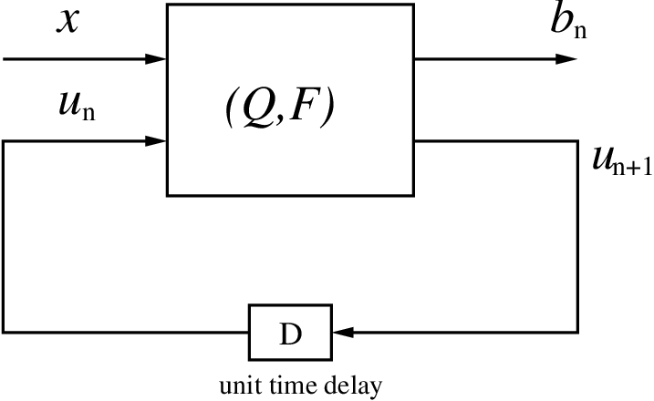
Let denote the set of possible “states” of the converter circuit that get updated after each iteration (clock cycle). More precisely, let
be a “quantizer” and let
be the map that determines the state of the circuit in the next clock cycle given its present state. After fixing the initial state of the circuit , the circuit employs the pair of functions to carry out the following iteration:
| (15) |
This procedure naturally defines a progressive family of encoders with the generator map given by
We will write to refer to the algorithmic converter defined by the pair and the implicit initial condition . If the generator is invertible (on ), then we say that the converter is invertible as well.
Definition 1 (1-bit quantizer).
We define the 1-bit quantizer with threshold value to be the function
| (16) |
Examples of algorithmic encoders
- 1.
Successive approximation algorithm for PCM. The successive approximation algorithm sets , and computes the bits , , in the binary expansion via the iteration
(17) Defining and , we obtain an invertible algorithmic converter for . A priori we can set , though it is easily seen that all the remain in .
- 2.
Beta-encoders with successive approximation implementation [7]. Let . A -representation of is an expansion of the form , where . Unlike a base-2 representation, almost every has infinitely many such representations. One class of expansions is found via the iteration
(18) where . The case corresponds to the “greedy” expansion, and the case to the “lazy” expansion. All values of are admissible in the sense that the remain bounded, which guarantees the validity of the inversion formula. Therefore the maps , and define an invertible algorithmic encoder for . It can be checked that all remain in a bounded interval independently of .
- 3.
First-order with constant input. Let . The first-order (Sigma-Delta) ADC sets the value of arbitrarily and runs the following iteration:
(19) It is easy to show that for all , and the boundedness of implies
(20) that is, the corresponding generator map is invertible. For this invertible algorithmic encoder, we have , , , and .
- 4.
th-order with constant input. Let be the forward difference operator defined by . A th-order ADC generalizes the scheme in Example 3 by replacing the first-order difference equation in (19) with
(21) which can be rewritten as
(22) where . Here is computed by a function of and the previous state variables , which must guarantee that the remain in some bounded interval for all , provided that the initial conditions are picked appropriately. If we define the vector state variable , then it is apparent that we can rewrite the above equations in the form
(23) where is the companion matrix defined by
(24) and . If is such that there exists a set with the property implies for each , then it is guaranteed that the are bounded, i.e., the scheme is stable. Note that any stable th order scheme is also a first order scheme with respect to the state variable . This implies that the inversion formula (20) holds, and therefore (23) defines an invertible algorithmic encoder. Stable schemes of arbitrary order have been devised in [13] and in [5]. For these schemes is a proper subinterval of .
II-C A Computational Model for Algorithmic Encoders and Formal Robustness
Next, we focus on a crucial property that is required for any ADC to be implementable in practice. As mentioned before, any ADC must perform certain arithmetic (computational) operations (e.g., addition, multiplication), and Boolean operations (e.g., comparison of some analog quantities with predetermined reference values). In the analog world, these operations cannot be done with infinite precision due to physical limitations. Therefore, the algorithm underlying a practical ADC needs to be robust with respect to implementation imperfections.
In this section, we shall describe a computational model for algorithmic encoders that includes all the examples discussed above and provides us with a formal framework in which to investigate others. This model will also allow us to formally define robustness for this class of encoders, and make comparisons with the state-of-the-art converters.
Directed Acyclic Graph Model
Recall (15) which (along with Figure 1) describes one cycle of an algorithmic encoder. So far, the pair of maps has been defined in a very general context and could have arbitrary complexity. In this section, we would like to propose a more realistic computational model for these maps. Our first assumption will be that and .
A directed acyclic graph (DAG) is a directed graph with no directed cycles. In a DAG, a source is a node (vertex) that has no incoming edges. Similarly, a sink is a node with no outgoing edges. Every DAG has a set of sources and a set of sinks, and every directed path starts from a source and ends at a sink. Our DAG model will always have source nodes that correspond to and the -dimensional vector , and sink nodes that correspond to and the -dimensional vector . This is illustrated in Figure 2 which depicts the DAG model of an implementation of the Golden Ratio Encoder (see Section III and Figure 4). Note that the feedback loop from Figure 1 is not a part of the DAG model, therefore the nodes associated to and have no incoming edges in Figure 2. Similarly the nodes associated to and have no outgoing edges. In addition, the node for , even when is not actually used as an input to , will be considered only as a source (and not as a sink).

In our DAG model, a node which is not a source or a sink will be associated with a component, i.e., a computational device with inputs and outputs. Mathematically, a component is simply a function (of smaller “complexity”) selected from a given fixed class. In the setting of this paper, we shall be concerned with only a restricted class of basic components: constant adder, pair adder/subtractor, constant multiplier, pair multiplier, binary quantizer, and replicator. These are depicted in Figure 3 along with their defining relations, except for the binary quantizer, which was defined in (16). Note that a component and the node at which it is placed should be consistent, i.e., the number of incoming edges must match the number of inputs of the component, and the number of outgoing edges must match the number of outputs of the component.

When the DAG model for an algorithmic encoder defined by the pair employs the ordered -tuple of components (including repetitions), we will denote this encoder by .

Robustness
We would like to say that an invertible algorithmic encoder is robust if is also invertible for any in a given neighborhood of and if the generator of has an inverse defined on that is also an inverse for the generator of . To make sense of this definition, we need to define the meaning of “neighborhood” of the pair .
Let us consider an algorithmic encoder as described above. Each component in may incorporate a vector of parameters (allowing for the possibility of the null vector). Let be the aggregate parameter vector of such an encoder. We will then denote by .
Let be a space of parameters for a given algorithmic encoder and consider a metric on . We now say that is robust if there exists a such that is invertible for all with with a common inverse. Similarly, we say that is robust in approximation if there exists a and a family such that
for all with , where .
From a practical point of view, if an algorithmic encoder is robust, and is implemented with a perturbed parameter instead of the intended , one can still obtain arbitrarily good approximations of the original analog object without knowing the actual value of . However, here we still assume that the “perturbed” encoder is algorithmic, i.e., we use the same perturbed parameter value at each clock cycle. In practice, however, many circuit components are “flaky”, that is, the associated parameters vary at each clock cycle. We can describe such an encoder again by (15), however we need to replace by , where is the sequence of the associated parameter vectors. With an abuse of notation, we denote such an encoder by (even though this is clearly not an algorithmic encoder in the sense of Section II-B). Note that if , i.e., for all , the corresponding encoder is . We now say that is strongly robust if there exists such that is invertible for all with with a common inverse. Here, is the space of parameter sequences for a given converter, and is an appropriate metric on . Similarly, we call an algorithmic encoder strongly robust in approximation if there exists and a family such that
for all flaky encoders with where is the metric on obtained by restricting (assuming such a restriction makes sense), is the N-tuple whose components are each , and .
Examples of Section II-B
Let us consider the examples of algorithmic encoders given in section II-B. The successive approximation algorithm is a special case of the beta encoder for and . As we mentioned before, there is no unique way to implement an algorithmic encoder using a given class of components. For example, given the set of rules set forth earlier, multiplication by could conceivably be implemented as a replicator followed by a pair adder (though a circuit engineer would probably not approve of this attempt). It is not our goal here to analyze whether a given DAG model is realizable in analog hardware, but to find out whether it is robust given its set of parameters.
The first order quantizer is perhaps the encoder with the simplest DAG model; its only parametric component is the binary quantizer, characterized by . For the beta encoder it is straightforward to write down a DAG model that incorporates only two parametric components: a constant multiplier and a binary quantizer. This model is thus characterized by the vector parameter . The successive approximation encoder corresponds to the special case . If the constant multiplier is avoided via the use of a replicator and adder, as described above, then this encoder would be characterized by , corresponding to the quantizer threshold.
These three models ( quantizer, beta encoder, and successive approximation) have been analyzed in [7] and the following statements hold:
- 1.
The successive approximation encoder is not robust for (with respect to the Euclidean metric on ). The implementation of successive approximation that avoids the constant multiplier as described above, and thus characterized by is not robust with respect to .
- 2.
The first order quantizer is strongly robust in approximation for the parameter value (and in fact for any other value for ). However, for .
- 3.
The beta encoder is strongly robust in approximation for a range of values of , when is fixed. Technically, this can be achieved by a metric which is the sum of the discrete metric on the first coordinate and the Euclidean metric on the second coordinate between any two vectors , and . This way we ensure that the first coordinate remains constant on a small neighborhood of any parameter vector. Here for . This choice of the metric however is not necessarily realistic.
- 4.
The beta encoder is not robust with respect to the Euclidean metric on the parameter vector space in which both and vary. In fact, this is the case even if we consider changes in only: let and be the generators of beta encoders with parameters and , respectively. Then and do not have a common inverse for any . To see this, let . Then a simple calculation shows
where for any . Consequently, .
This shows that to decode a beta-encoded bit-stream, one needs to know the value of at least within the desired precision level. This problem was addressed in [8], where a method was proposed for embedding the value of in the encoded bit-stream in such a way that one can recover an estimate for (in the digital domain) with exponential precision. Beta encoders with the modifications of [8] are effectively robust in approximation (the inverse of the generator of the perturbed encoder is different from the inverse of the intended encoder, however it can be precisely computed). Still, even with these modifications, the corresponding encoders are not strongly robust with respect to the parameter .
- 5.
The stable schemes of arbitrary order that were designed by Daubechies and DeVore, [13], are strongly robust in approximation with respect to their parameter sets. Also, a wide family of second-order schemes, as discussed in [14], are strongly robust in approximation. On the other hand, the family of exponentially accurate one-bit schemes reported in [5] are not robust because each scheme in this family employs a vector of constant multipliers which, when perturbed arbitrarily, result in bit sequences that provide no guarantee of even mere invertibility (using the original decoder). The only reconstruction accuracy guarantee is of Lipshitz type, i.e. the error of reconstruction is controlled by a constant times the parameter distortion.
Neither of these cases result in an algorithmic encoder with a DAG model that is robust in its full set of parameters and achieves exponential accuracy. To the best of our knowledge, our discussion in the next section provides the first example of an encoder that is (strongly) robust in approximation while simultaneously achieving exponential accuracy.
III The Golden Ratio Encoder
In this section, we introduce a Nyquist rate ADC, the golden ratio encoder (GRE), that bypasses the robustness concerns mentioned above while still enjoying exponential accuracy in the bit-rate. In particular, GRE is an algorithmic encoder that is strongly robust in approximation with respect to its full set of parameters, and its accuracy is exponential. The DAG model and block diagram of the GRE are given in Figures 2 and 4, respectively.
III-A The scheme
We start by describing the recursion underlying the GRE. To quantize a given real number , we set and , and run the iteration process
| (25) |
Here, is a quantizer to be specified later. Note that (25) describes a piecewise affine discrete dynamical system on . More precisely, define
| (26) |
Then we can rewrite (25) as
| (27) |
Now, let , , and suppose is a quantizer on . The formulation in (27) shows that GRE is an algorithmic encoder, , where for . Next, we show that GRE is invertible by establishing that, if is chosen appropriately, the sequence obtained via (25) gives a beta representation of with .
III-B Approximation Error and Accuracy
Proposition 1.
Let and suppose are generated via (25) with and . Then
if and only if the state sequence is bounded. Here is the golden mean.
Proof:
Note that
| (28) | |||||
where the third equality follows from , and the last equality is obtained by setting and . Defining the -term approximation error to be e_N(x) := x - ∑_n=0^N-1 b_n ϕ^-n= ϕ^-N(u_N + ϕ u_N+1) it follows that lim_N→∞ e_N(x) = 0, provided
| (29) |
Clearly, (29) is satisfied if there is a constant , independent of , such that , . Conversely, suppose (29) holds, and assume that is unbounded. Let N be the smallest integer for which for some . Without loss of generality, assume (the argument below, with simple modifications, applies if ). Then, using (25) repeatedly, one can show that u_N+k¿C’ϕ^3 f_k-1 - f_k+2+1 where is the th Fibonacci number. Finally, using f_k= ϕ k -(1-ϕ) k 5 (which is known as Binet’s formula, e.g., see [15]) we conclude that for every positive integer , showing that (29) does not hold if the sequence is not bounded.
∎
Note that the proof of Proposition 1 also shows that the -term approximation error decays exponentially in if and only if the state sequence , obtained when encoding , remains bounded by a constant (which may depend on ). We will say that a GRE is stable on if the constant in Proposition 1 is independent of , i.e., if the state sequences with and are bounded by a constant uniformly in . In this case, the following proposition holds.
Proposition 2.
Let be the generator of the GRE, described by (25). If the GRE is stable on , it is exponentially accurate on . In particular, .
Next, we investigate quantizers that generate stable encoders.
III-C Stability and robustness with respect to imperfect quantizers
To establish stability, we will show that for several choices of the quantizer , there exist bounded positively invariant sets such that . We will frequently use the basic 1-bit quantizer,
Most practical quantizers are implemented using arithmetic operations and . One class that we will consider is given by
| (30) |
Note that in the DAG model of GRE, the circuit components that implement incorporate a parameter vector . Here, is the threshold of the 1-bit basic quantizer, and is the gain factor of the multiplier that maps to . One of our main goals in this paper is to prove that GRE, with the implementation depicted in Figure 4, is strongly robust in approximation with respect to its full set of parameters. That is, we shall allow the parameter values to change at each clock cycle (within some margin). Such changes in parameter can be incorporated to the recursion (25) by allowing the quantizer to be flaky. More precisely, for , let be the flaky version of defined by
We shall denote by the flaky version of , which is now
Note that (25), implemented with , does not generate an algorithmic encoder. At each clock cycle, the action of is identical to the action of for some . In this case, using the notation introduced before, (25) generates . We will refer to this encoder family as GRE with flaky quantizer.
III-C1 A stable GRE with no multipliers: the case
We now set in (30) and show that the GRE implemented with is stable, and thus generates an encoder family with exponential accuracy (by Proposition 2). Note that in this case, the recursion relation (25) does not employ any multipliers (with gains different from unity). In other words, the associated DAG model does not contain any “constant multiplier” component.
Proposition 3.
Consider , defined as in (26). Then satisfies
Proof:
By induction. It is easier to see this on the equivalent recursion (25). Suppose , i.e., and are in . Then is in , which concludes the proof. ∎
It follows from the above proposition that the GRE implemented with is stable whenever the initial state , i.e., . In fact, one can make a stronger statement because a longer chunk of the positive real axis is in the basin of attraction of the map .
Proposition 4.
The GRE implemented with is stable on , where is the golden mean. More precisely, for any , there exists a positive integer such that for all .
Corollary 5.
Let , set , , and generate the bit sequence by running the recursion (25) with . Then, for ,
One can choose uniformly in in any closed subset of . In particular, for all .
Remarks.
- 1.
The proofs of Proposition 4 and Corollary 5 follow trivially from Proposition 3 when . It is also easy to see that for , i.e., after one iteration the state variables and are both in . Furthermore, it can be shown that
where denotes the th Fibonacci number. We do not include the proof of this last statement here, as the argument is somewhat long, and the result is not crucial from the viewpoint of this paper.
- 2.
In this case, i.e., when , the encoder is not robust with respect to quantizer imperfections. More precisely, if we replace with , with , then can grow regardless of how small is. This is a result of the mixing properties of the piecewise affine map associated with GRE. In particular, one can show that , where is the set of points whose th forward image is outside the unit square. Figure 5 shows the fraction of 10,000 randomly chosen -values for which as a function of . In fact, suppose with and . Then, the probability that is outside of is , which is superior to the case with PCM where the corresponding probability scales like . This observation suggests that “GRE with no multipliers”, with its simply-implementable nature, could still be useful in applications where high fidelity is not required. We shall discuss this in more detail elsewhere.

III-C2 Other values of : stable and robust GRE
In the previous subsection, we saw that GRE, implemented with , , is stable on , and thus enjoys exponential accuracy; unfortunately, the resulting algorithmic encoder is not robust. In this subsection, we show that there is a wide parameter range for and for which the map with has positively invariant sets that do not depend on the particular values of and . Using such a result, we then conclude that, with the appropriate choice of parameters, the associated GRE is strongly robust in approximation with respect to , the quantizer threshold, and , the multiplier needed to implement . We also show that the invariant sets can be constructed to have the additional property that for a small value of one has , where denotes the open ball around 0 with radius . In this case, depends on . Consequently, even if the image of any state is perturbed within a radius of , it still remains within . Hence we also achieve stability under small additive noise or arithmetic errors.
Lemma 6.
Let . There is a set , explicitly given in (32), and a wide range for parameters , and such that .
Proof:
Our proof is constructive. In particular, for a given , we obtain a parametrization for , which turns out to be a rectangular set. The corresponding ranges for , and are also obtained implicitly below. We will give explicit ranges for these parameters later in the text.
Our construction of the set , which only depends on , is best explained with a figure. Consider the two rectangles and in Figure 6. These rectangles are designed to be such that their respective images under the linear map , and the affine map , defined by
| (31) |
are the same, i.e., .

The rectangle is such that its -neighborhood is contained within the union of and . This guards against additive noise. The fact that the rectangles and overlap (the shaded region) allows for the use of a flaky quantizer. Call this region . As long as the region in which the quantizer operates in the flaky mode is a subset of , and on and on , it follows that . It is then most convenient to choose and we clearly have . Note that if , any choice , and for which the graph of remains inside the shaded region for will ensure .
Next, we check the existence of at least one solution to this setup. This can be done easily in terms the parameters defined in the figure. First note that the linear map has the eigenvalues and with corresponding (normalized) eigenvectors and . Hence acts as an expansion by a factor of along , and reflection followed by contraction by a factor of along . is the same as followed by a vertical translation of . It follows after some straightforward algebraic calculations that the mapping relations described above imply
Consequently, the positively invariant set is the set of all points inside the rectangle where
| (32) |
Note that depends only on . Moreover, the existence of the overlapping region is equivalent to the condition which turns out to be equivalent to μ¡ 1 2ϕ 2 ϕ+2 ≈0.1004. ∎
Flaky quantizers, linear thresholds
Next we consider the case and specify ranges for , and such that .
Proposition 7.
Let and such that
| (33) |
be fixed. Define
| (34) | |||||
| (35) |
If , then for every .

Remarks.
- 1.
The dark line segment depicted in Figure 6 within the overlapping region , refers to a hypothetical quantizer threshold that is allowed to vary within . Proposition 7 essentially determines the vertical axis intercepts of lines with a given slope, , the corresponding segments of which remain in the overlapping region . The proof is straightforward but tedious, and will be omitted.
- 2.
- 3.
For any , note that is invertible at and set
Then, for any , we have
provided
Note also that for any , we have . Thus,
if . Consequently, we observe that
for any and .
- 4.
We can also determine the allowed range for , given the range for , by reversing the argument above. The extreme values of and are
(36) (37) For any in the open interval between these extreme values, set
Then, for any , is in the allowed region where
(38) (39) This is shown in Figure 7. Consequently, we observe that GRE implemented with remains stable for any and provided and .
- 5.
For the case , the expressions above simplify significantly. In (33), and . Consequently, the extreme values and are 1 and 2, respectively. One can repeat the calculations above to derive the allowed ranges for the parameters to vary. Observe that gives the widest range for the parameters. This can be seen in Figure 7.
We now go back to the GRE and state the implications of the results obtained in this subsection. The recursion relations (25) that define GRE assume perfect arithmetic. We modify (25) to allow arithmetic imperfections, e.g., additive noise, as follows
| (40) |
and conclude this section with the following stability theorem.
Theorem 8.
Proof:
This immediately follows from our remarks above. In particular, given , choose such that the corresponding . By monotonicity of both and , any will do. Next, choose some , and set . The statement of the theorem now holds with and . ∎
When , i.e., when we assume the recursion relations (25) are implemented without an additive error, Theorem 8 implies that GRE is strongly robust in approximation with respect to the parameter , and . More precisely, the following corollary holds.
Corollary 9.
Let , and . There exist , and such that , generated via (25) with , , and , approximate exponentially accurately whenever . In particular, the -term approximation error satisfies
where .
III-D Effect of additive noise and arithmetic errors on reconstruction error
Corollary 9 shows that the GRE is robust with respect to quantizer imperfections under the assumption that the recursion relations given by (25) are strictly satisfied. That is, we have quite a bit of freedom in choosing the quantizer , assuming the arithmetic, i.e., addition, can be done error-free. We now investigate the effect of arithmetic errors on the reconstruction error. To this end, we model such imperfections as additive noise and, as before, replace (25) with (40), where denotes the additive noise. While Theorem 8 shows that the encoder is stable under small additive errors, the reconstruction error is not guaranteed to become arbitrarily small with increasing number of bits. This is observed in Figure 8 where the system is stable for the given imperfection parameters and noise level, however the reconstruction error is never better than the noise level.

Note that for stable systems, we unavoidably have
| (41) |
where the “noise term” in (41) does not vanish as tends to infinity. To see this, define . If we assume to be i.i.d. with mean 0 and variance , then we have
Hence we can conclude from this the -independent result
In Figure 8, we incorporated uniform noise in the range . This would yield , hence the saturation of the root-mean-square-error (RMSE) at . Note, however, that the figure was created with an average over 10,000 randomly chosen values. Although independent experiments were not run for the same values of , the -independence of the above formula enables us to predict the outcome almost exactly.
In general, if is the probability density function for each , then will converge to a random variable the probability density function of which has Fourier transform given by the convergent infinite product
III-E Bias removal for the decoder
Due to the nature of any ‘cautious’ beta-encoder, the standard -bit decoder for the GRE yields approximations that are biased, i.e., the error has a non-zero mean. This is readily seen by the error formula
which implies that for all and . Note that all points in the invariant rectangle satisfy .
This suggests adding a constant (-independent) term to the standard -bit decoding expression to minimize . Various choices are possible for the norm. For the -norm, should be chosen to be average value of the minimum and the maximum values of . For the -norm, should be the median value and for the -norm, should be the mean value of . Since we are interested in the -norm, we will choose via
where is the range of values and we have assumed uniform distribution of values.
This integral is in general difficult to compute explicitly due to the lack of a simple formula for . One heuristic that is motivated by the mixing properties of the map is to replace the average value by . If the set of initial conditions did not have zero two-dimensional Lebesgue measure, this heuristic could be turned into a rigorous result as well.
However, there is a special case in which the bias can be computed explicitly. This is the case and . Then the invariant set is and
where denotes the coordinate-wise fractional part operator on any real vector. Since for all non-zero integers , it follows that for all . Hence setting , we find
It is also possible to compute the integral explicitly when and for some . In this case it can be shown that the invariant set is the union of at most 3 rectangles whose axes are parallel to and . We omit the details.
III-F Circuit implementation: Requantization
As we mentioned briefly in the introduction, A/D converters (other than PCM) typically incorporate a requantization stage after which the more conventional binary (base-2) representations are generated. This operation is close to a decoding operation, except it can be done entirely in digital logic (i.e., perfect arithmetic) using the bitstreams generated by the specific algorithm of the converter. In principle sophisticated digital circuits could also be employed.
In the case of the Golden Ratio Encoder, it turns out that a fairly simple requantization algorithm exists that incorporates a digital arithmetic unit and a minimum amount of memory that can be hardwired. The algorithm is based on recursively computing the base-2 representations of powers of the golden ratio. In Figure 9, denotes the -bit base-2 representation of . Mimicking the relation , the digital circuit recursively sets
which then gets multiplied by and added to , where
The circuit needs to be set up so that is the expansion of in base 2, accurate up to at least bits, in addition to the initial conditions and . To minimize round-off errors, could be taken to be a large number (much larger than , which determines the output resolution).

IV Higher order schemes: Tribonacci and Polynacci encoders
What made the Golden Ratio Encoder (or the ‘Fibonacci’ Encoder) interesting was the fact that a beta-expansion for was attained via a difference equation with coefficients, thereby removing the necessity to have a perfect constant multiplier. (Recall that multipliers were still employed for the quantization operation, but they no longer needed to be precise.)
This principle can be further exploited by considering more general difference equations of this same type. An immediate class of such equations are suggested by the recursion
where is some integer. For , one gets the Fibonacci sequence if the initial condition is given by , . For , one gets the Tribonacci sequence when , . The general case yields the Polynacci sequence.
For bit encoding of real numbers, one then sets up the iteration
| (42) |
with the initial conditions , . In -dimensions, the iteration can be rewritten as
| (43) |
It can be shown that the characteristic equation
has its largest root in the interval and all remaining roots inside the unit circle (hence is a Pisot number). Moreover as , one has monotonically.
One is then left with the construction of quantization rules that yield bounded sequences . While this is a slightly more difficult task to achieve, it is nevertheless possible to find such quantization rules. The details will be given in a separate manuscript.
The final outcome of this generalization is the accuracy estimate
whose rate becomes asymptotically optimal as .
V Acknowledgments
We would like to thank Felix Krahmer, Rachel Ward, and Matt Yedlin for various conversations and comments that have helped initiate and improve this paper.
Ingrid Daubechies gratefully acknowledges partial support by the NSF grant DMS-0504924. Sinan Güntürk has been supported in part by the NSF Grant CCF-0515187, an Alfred P. Sloan Research Fellowship, and an NYU Goddard Fellowship. Yang Wang has been supported in part by the NSF Grant DMS-0410062. Özgür Yılmaz was partly supported by a Discovery Grant from the Natural Sciences and Engineering Research Council of Canada. This work was initiated during a BIRS Workshop and finalized during an AIM Workshop. The authors greatfully acknowledge the Banff International Research Station and the American Institute of Mathematics.
References
- [1] H. Inose and Y. Yasuda, “A unity bit coding method by negative feedback,” Proceedings of the IEEE, vol. 51, no. 11, pp. 1524–1535, 1963.
- [2] J. Candy and G. Temes, “Oversampling Delta-Sigma Data Converters: Theory, Design and Simulation,” IEEE Press, New York, 1992.
- [3] R. Schreier and G. Temes, Understanding delta-sigma data converters. John Wiley & Sons, 2004.
- [4] C. Güntürk, J. Lagarias, and V. Vaishampayan, “On the robustness of single-loop sigma-delta modulation,” IEEE Transactions on Information Theory, vol. 47, no. 5, pp. 1735–1744, 2001.
- [5] C. Güntürk, “One-bit sigma-delta quantization with exponential accuracy,” Communications on Pure and Applied Mathematics, vol. 56, no. 11, pp. 1608–1630, 2003.
- [6] K. Dajani and C. Kraaikamp, “From greedy to lazy expansions and their driving dynamics,” Expositiones Mathematicae, vol. 20, no. 4, pp. 315–327, 2002.
- [7] I. Daubechies, R. DeVore, C. Güntürk, and V. Vaishampayan, “A/D conversion with imperfect quantizers,” IEEE Transactions on Information Theory, vol. 52, no. 3, pp. 874–885, March 2006.
- [8] I. Daubechies and Ö. Yılmaz, “Robust and practical analog-to-digital conversion with exponential precision,” IEEE Transactions on Information Theory, vol. 52, no. 8, August 2006.
- [9] A. Karanicolas, H. Lee, and K. Barcrania, “A 15-b 1-Msample/s digitally self-calibrated pipeline ADC,” IEEE Journal of Solid-State Circuits, vol. 28, no. 12, pp. 1207–1215, 1993.
- [10] W. Parry, “On the -expansions of real numbers,” Acta Mathematica Hungarica, vol. 11, no. 3, pp. 401–416, 1960.
- [11] N. Sidorov, “Almost Every Number Has a Continuum of -Expansions,” American Mathematical Monthly, vol. 110, no. 9, pp. 838–842, 2003.
- [12] A. N. Kolmogorov and V. M. Tihomirov, “-entropy and -capacity of sets in functional space,” Amer. Math. Soc. Transl. (2), vol. 17, pp. 277–364, 1961.
- [13] I. Daubechies and R. DeVore, “Reconstructing a bandlimited function from very coarsely quantized data: A family of stable sigma-delta modulators of arbitrary order,” Annals of Mathematics, vol. 158, no. 2, pp. 679–710, 2003.
- [14] Ö. Yılmaz, “Stability analysis for several second-order sigma-delta methods of coarse quantization of bandlimited functions,” Constructive approximation, vol. 18, no. 4, pp. 599–623, 2002.
- [15] N. Vorobiev, Fibonacci Numbers. Birkhäuser, 2003.