Groundstatable fermionic wavefunctions and their associated many-body Hamiltonians

Daniel Charrier^1,2 Affiliation: ¹ Physics Department, Boston University, Boston, MA 02215, USA
² Laboratoire de Physique Théorique, IRSAMC, UPS and CNRS, Université de Toulouse, F-31062 Toulouse, France Claudio Chamon¹ Affiliation: ¹ Physics Department, Boston University, Boston, MA 02215, USA
² Laboratoire de Physique Théorique, IRSAMC, UPS and CNRS, Université de Toulouse, F-31062 Toulouse, France

August 24, 2026

Abstract

In the vast majority of many-body problems, it is the kinetic energy part of the Hamiltonian that is best known microscopically, and it is the detailed form of the interactions between the particles, the potential energy term, that is harder to determine from first principles. An example is the case of high temperature superconductors: while a tight-binding model captures the kinetic term, it is not clear that there is superconductivity with only an onsite repulsion and, thus, that the problem is accurately described by the Hubbard model alone. Here we pose the question of whether, once the kinetic energy is fixed, a candidate ground state is groundstatable or not. The easiness to answer this question is strongly related to the presence or the absence of a sign problem in the system. When groundstatability is satisfied, it is simple to obtain the potential energy that will lead to such a ground state. As a concrete case study, we apply these ideas to different fermionic wavefunctions with superconductive or spin-density wave correlations and we also study the influence of Jastrow factors. The kinetic energy considered is a simple next nearest neighbor hopping term.

pacs

71.10.Fd, 74.20.Fg, 02.70.Tt

I Introduction

The problem of finding the ground state of a many-particle Hamiltonian is, in general, a daunting task. The problem is most severe in the case of fermionic particles, where the infamous fermion sign problem plagues solutions via numerical methods. In contrast, in bosonic systems, Monte Carlo methods are rather efficient in simulating systems of reasonably large sizes. Certain methods, such as Density Matrix Renormalization Group, avoid the sign problem, but are mainly restricted to 1d or quasi-1d systems.

In this paper we step back from the problem of determining the ground state of a given many-body Hamiltonian, and instead pose the following question: fixing the kinetic energy part of the Hamiltonian, can a given wavefunction be the ground state for some choice of potential energy? Put simply, we ask if the wavefunction is groundstatable. The question is trivial to answer for bosonic system, as we discuss below, but in the case of fermions it is much more difficult and subtle.

To illustrate this idea, let us start with a very simple example: the case of a single spin $1/2$ degree of freedom. Consider a Hamiltonian of the form:

\hat{H}=-\hat{\sigma}_{x}+\hat{V}_{\alpha},

(1)

where $\hat{\sigma}_{x}$ is the usual spin-flip operator and $\hat{V}_{\alpha}$ is a diagonal operator in the $\{|\!\!\uparrow\rangle,|\!\!\downarrow\rangle\}$ basis. Here, we will not specify $\hat{V}_{\alpha}$ and try to diagonalize $\hat{H}$ ; instead , we will consider the wavefunction

|\Psi_{\alpha}\rangle=\frac{1}{\sqrt{2(1+\alpha^{2})}}\left[(1-\alpha)\;|\!\!\uparrow\rangle+(1+\alpha)\;|\!\!\downarrow\rangle\right]

(2)

and ask what the condition is on $\alpha$ so that $|\Psi_{\alpha}\rangle$ is the ground state of $\hat{H}$ , for some a proper choice of $\hat{V}_{\alpha}$ . To answer that, the first step is to make $|\Psi_{\alpha}\rangle$ an eigenstate of $\hat{H}$ by imposing $\hat{H}|\Psi_{\alpha}\rangle=0$ (so $|\Psi_{\alpha}\rangle$ is an eigenstate of $\hat{H}$ with energy zero). The expression of $\hat{V}_{\alpha}$ follows immediately and we can rewrite $\hat{H}$ in a matrix form as:

\hat{H}=\left(\begin{array}[]{cc}\!\!\!\frac{1+\alpha}{1-\alpha}&-1\\ -1&\frac{1-\alpha}{1+\alpha}\end{array}\right).

(3)

The two eigenvalues of this problem are $\lambda_{1}=0$ and $\lambda_{2}=\frac{1+\alpha}{1-\alpha}+\frac{1-\alpha}{1+\alpha}$ . Now, it is easy to see that $|\Psi_{\alpha}\rangle$ will be the ground state of $\hat{H}$ if and only if $\alpha<1$ (i.e. if the wavefunction elements are all positive). We will say that $|\Psi_{\alpha}\rangle$ is groundstatable for $\alpha<1$ . On the contrary, when $\alpha>1$ , $|\Psi_{\alpha}\rangle$ is an excited state of the problem and no longer groundstatable. At the boundary between the two cases, one component of the wavefunction vanishes at $\alpha=1$ . Then, the potential energy blows up and the eigenvalue $\lambda_{2}$ goes from $+\infty$ to $-\infty$ . Of course, the property of groundstatability for a given wavefunction is directly related to the kinetic energy operator we have considered. Had we chosen a different operator, we would have reached a different conclusion on $\alpha$ . The point is that once this operator is fixed, the problem is uniquely defined.

This approach to the single spin Hamiltonian can be extended to a many-body problem, where the kinetic energy is often chosen to be a local hopping operator between nearby sites. Then, from the set of all possible many-body wavefunctions, some are groundstatable and others are not. It is of crucial importance to establish in which category a given wavefunction belongs to, since it determines if this state is allowed in nature. In general, for a given kinetic energy term, the Hilbert space is broken down in regions in which the wavefunction satisfies groundstatability; as we will see below, the level of complexity of the partitions of the space into such regions is closely related to the presence or the absence of a sign problem in the Hamiltonian.

The paper is organized as follows. In section II we define the problem of groundstatability on a finite dimensional Hilbert space and we show how it can be solved on a particular case where the Hamiltonian admits a product form. Then, we present in section III the main part of our work, namely how one can build a Hamiltonian for which a given many-body fermionic wavefunction is the groundstate. The numerical procedure is also detailed in that section. Results are shown in section IV. We discuss the case of the wavefunction for non-interacting fermions which allows us to illustrate the loss of groundstatability in these systems. We then present the potentials obtained from mean-field solutions of the Hubbard model, BCS superconductors and spin-density waves (SDW). These results are in accordance with mean-field analysis. By considering additional Jastrow factors, we also examine partially-projected BCS wavefunctions relevant for the study of high- $T_{c}$ superconductors. Finally, a more open problem, with a class of wavefunctions containing both superconductivity and antiferromagnetism, is investigated.

II The problem

II.1 General considerations

Let us consider a finite dimensional matrix example. Take a Hamiltonian matrix $H_{C,C^{\prime}}$ , where $C,C^{\prime}$ index the states in the $d_{H}$ -dimensional Hilbert space, for example the spatial configurations of fermions on a finite lattice. Suppose that the off-diagonal elements $H_{C\neq C^{\prime}}$ are known, and one wants to determine if the vector (state) with components $\Psi_{C}$ can be the ground state if the matrix elements in the diagonal are properly picked. There are two steps in the problem: the first is trivial, to make $|\Psi\rangle$ an eigenstate, and the second is the problem we pose, whether it can be the ground state.

We start by determining the diagonal elements from the condition that $|\Psi\rangle$ is an eigenstate. For simplicity, we shift again the eigenvalue $\lambda_{\Psi}$ to zero, and solve for the $d_{H}$ variables $H_{CC}$ in the diagonal:

\sum_{C^{\prime}}\;H_{CC^{\prime}}\;\Psi_{C^{\prime}}=0\;\Rightarrow\;H_{CC}=-\sum_{C^{\prime}\neq C}\;H_{CC^{\prime}}\;\frac{\Psi_{C^{\prime}}}{\Psi_{C}}\;,

(4)

so the Hamiltonian can be written as

	$\displaystyle\hat{H}=-\frac{1}{2}\sum_{C\neq C^{\prime}}H_{CC^{\prime}}\;\Big[\frac{\Psi_{C^{\prime}}}{\Psi_{C}}\|C\rangle\langle C\|+\frac{\Psi_{C}}{\Psi_{C^{\prime}}}\|C^{\prime}\rangle\langle C^{\prime}\|$		(5)
	$\displaystyle-\|C\rangle\langle C^{\prime}\|-\|C^{\prime}\rangle\langle C\|\Big]\;,$

which is a sum of projector operators acting on a 2-dimensional subspace of states $C,C^{\prime}$ (one can check that the operator within brackets squares to a multiple of itself).

The problem of groundstatability is that it is not guaranteed, with the Hamiltonian $H_{CC^{\prime}}$ now determined, that $|\Psi\rangle$ is the ground state, and not an excited state. What are the conditions on the vector components $\Psi_{C}$ for it to be the ground state? If the off-diagonal matrix elements are all non-positive, then one can make use of the Perron-Frobenius theorem and the well-known connection to stochastic dynamics [1], or alternatively cast the Hamiltonian as a sum of positive semi-definite projectors [2]. Basically, the condition of groundstatability in this case is that $\Psi_{C}>0$ , $\forall C$ . This is the case of matrix Hamiltonians for bosonic systems, and the strictly negative or zero off-diagonal elements is related to the absence of a sign-problem in the Hamiltonian. The problem of the single spin $1/2$ mentioned in the introduction falls in this category. Now, one does not have the luxury of the stochastic mapping to a problem with positive probabilities in general. If some off-diagonal elements of the Hamiltonian are non positive, we lack any general theorem to conclude on the groundstatability of the wavefunction. Sometimes, it is possible to find a gauge transformation to come back to the simpler case with all strictly negative or zero off-diagonal elements; this happens for some spin models, like the anti-ferromagnetic Heisenberg Hamiltonian, where the sign structure of the ground state is given by the Marshall rule [3]. However, in fermionic problems and some frustrated magnets, the problem remains unsolved.

II.2 Hamiltonians with a separable form

Before going to our main case of interest which is the fermionic Hamiltonian with neighboring site hopping for kinetic energy term, we would like to present another class of models where the question of groundstatability can be completely and analytically answered even in the absence of a Marshall-like rule. The problem of groundstatability is defined for a given choice of kinetic energy operator, and we will choose here the off-diagonal elements of the Hamiltonian $H^{(\pm)}_{C\neq C^{\prime}}=\pm w_{C}w_{C^{\prime}}$ to be separable into products of $w_{C},w_{C^{\prime}}\in\mathbb{R}$ . Notice that these models are highly non-local problems. However, they are interesting because they display the fundamental difference between the presence/absence of a sign problem in the system, mainly, the parameter space can be separated into disconnected groundstatable regions in the $(+)$ case, whereas in the $(-)$ case the groundstatable region is just made of a single block.

Let us consider the two possibilities: $H^{(+)}_{C\neq C^{\prime}}=+w_{C}w_{C^{\prime}}$ or $H^{(-)}_{C\neq C^{\prime}}=-w_{C}w_{C^{\prime}}$ . Now, given a vector $\Psi_{C}$ , we construct the diagonal elements according to Eq. (4) so that $\Psi_{C}$ is an eigenvector with eigenvalue zero. The Schrödinger equation for any eigenstate $|\psi^{\lambda}\rangle=\sum_{C}\psi^{\lambda}_{C}\;|C\rangle$ with energy $\lambda$ reads:

\pm\sum_{C\neq C^{\prime}}w_{C}w_{C^{\prime}}\;\psi^{\lambda}_{C^{\prime}}=\left(\lambda\pm\sum_{C\neq C^{\prime}}w_{C}w_{C^{\prime}}\frac{\Psi_{C^{\prime}}}{\Psi_{C}}\right)\psi^{\lambda}_{C}

(6)

and it is then straightforward to show that all eigenvalues $\lambda$ are solutions of the equation:

f_{\pm}(\lambda)=\sum_{C}\frac{w_{C}^{2}}{\lambda\pm\left(\sum_{C^{\prime}}w_{C^{\prime}}\Psi_{C^{\prime}}\right)w_{C}/\Psi_{C}}=\pm 1.

(7)

$\lambda=0$ is indeed, by construction, a solution. The state $|\Psi\rangle$ is the ground state if all other solutions of Eq. (7) are positive. It follows that solutions of $f_{-}(\lambda)=-1$ satisfy $\lambda\geq 0$ if all poles of the function $f_{-}(\lambda)$ are positive, and solutions of $f_{+}(\lambda)=+1$ satisfy $\lambda\geq 0$ if one and only one of the poles of the function $f_{+}(\lambda)$ is negative (see Figure 1).

Refer to caption — Figure 1: (color online) Solutions of the Schrödinger equation (7) (circles) for a three dimensional Hilbert space when $\lambda=0$ is the ground state energy. Notice the positions of the poles with respect to zero in the two cases.

Notice that in the ( $-$ ) case, to fix the poles of $f_{-}(\lambda)$ to be positive, the signs of groundstatable vectors $\Psi_{C}$ are related to those of $w_{C}$ , and one can thus write $\Psi_{C}={\rm sgn}(w_{C})\,|\Psi_{C}|$ , which is a simple example of a Marshall sign. In this case, the signs of the $w_{C}$ ’s can be gauged away from the Hamiltonian, bringing it to the form that satisfy the Perron-Frobenius theorem: $H_{C\neq C^{\prime}}\to\tilde{H}_{C\neq C^{\prime}}=-|w_{C}||w_{C}^{\prime}|$ and $\Psi_{C}\to\tilde{\Psi}_{C}=|\Psi_{C}|>0$ .

The condition for groundstatability in the ( $+$ ) case is richer. The condition that one and only one of the poles of the function $f_{+}(\lambda)$ is negative leads to $d_{H}$ distinct sectors in the Hilbert space, each sector corresponding to the choice of which of the $d_{H}$ poles is selected to be the negative one. More explicitly, the condition on the poles is equivalent, for $\Psi_{C}\neq 0$ , to:

	$\displaystyle w_{\bar{C}}\Psi_{\bar{C}}/(\sum_{C^{\prime}}w_{C^{\prime}}\Psi_{C^{\prime}})$	$\displaystyle>$	$\displaystyle 0\,\,\mathrm{for}\ \bar{C}$		(8)
	$\displaystyle w_{C}\Psi_{C}/(\sum_{C^{\prime}}w_{C^{\prime}}\Psi_{C^{\prime}})$	$\displaystyle<0$	$\displaystyle\,\,\mathrm{for}\,\,C\neq\bar{C}$		(9)

Each of these inequalities split the Hilbert space into two pieces via a hyperplane, and the $d_{H}$ conditions lead to a simplex, and the choices of the $\bar{C}$ to $d_{H}$ such simplexes (see Fig. 2 for simple examples on $3\times 3$ Hamiltonians).

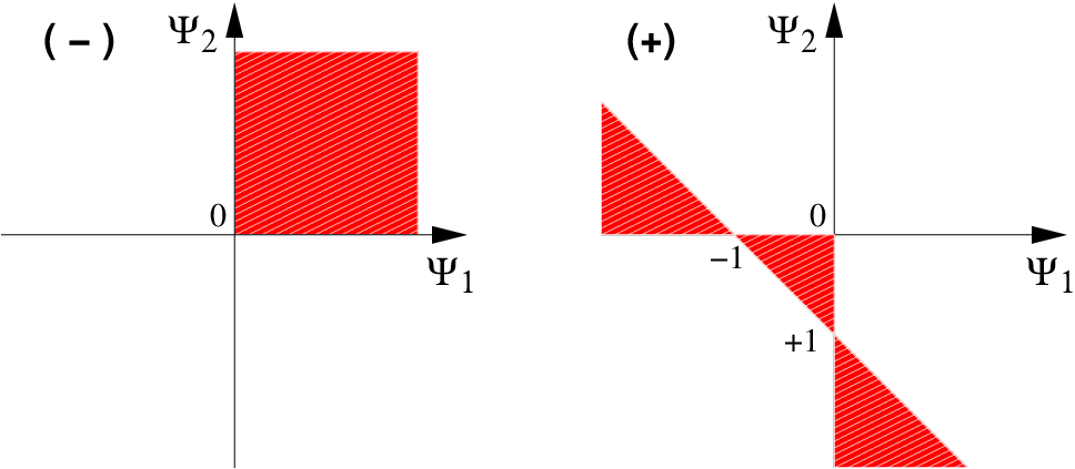
In most of the cases, the edges of the simplexes correspond to the vanishing of one of the $\Psi_{C}$ in the wavefunction. Indeed, coming from a groundstatable region, if one component $\Psi_{C}$ changes sign the inequalities (9) are violated. On the edge, $\Psi_{C}=0$ , the associated diagonal element $H_{CC}$ is infinite [see Eq. (4)] and one of the positive eigenvalues diverges towards $+\infty$ and reappears at $-\infty$ . Another edge is given by the equation $\sum w_{C}\Psi_{C}=0$ . In this case, the whole hamiltonian is reduced to the projector $\hat{H}=|w\rangle\langle w|$ (this corresponds to the diagonal line on Fig. 2) and there are only two eigenvalues: $0$ and $1$ . From this point of view, boundaries between groundstatable and non-groundstatable either corresponds to ill-defined Hamiltonians or to highly degenerate problems, the first case being the most common one.

For a Hamiltonian with off-diagonal matrix elements that cannot be separated into a product as in the example above, the situation is more complicated. Nonetheless, one should expect that the feature we encountered in the simple case study should remain: generically the set of groundstatable wavefunctions within the Hilbert space is largely fragmented into regions. In the case of the example, there are order $d_{H}$ , the dimension of the Hilbert space, regions. This is to be contrasted to the case where there is no fermion sign problem, where there is one single region. This fragmentation of the groundstatable set should be a generic feature of systems with fermionic sign problems. Moreover, we also expect the diagonal part of the Hamiltonian to abruptly change form when it leaves a groundstatable region and to become singular at the boundary (the edges of the simplexes). These abrupt changes in the Hamiltonian can be used as telltales that the wavefunction, as function of some parameter, exits a groundstatable region.

It is important to point out that, within a given groundstatable region, many phases of matter can exist. Order parameters computed from a groundstatable wavefunction can be used to classify the phases. The groundstatable regions thus do not delimit single phases; what they do demarcate are the regions where a wavefunction can possibly correspond to a state of matter, for a fixed kinetic energy term in the Hamiltonian.

III Many-body fermionic Hamiltonians

Let us now turn into a more practical application, and show how one can implement the procedure of finding the potential energy term for which a given fermionic many-body state $|\Psi\rangle$ is the ground state, given a kinetic energy. We will consider specifically the case where the kinetic energy comes from a tight-binding hopping term on a lattice, which is common in many strongly-correlated electronic problems. We consider the case of fermions on a square lattice, and detail below the numerical procedure used to evaluate the potential energy of the Hamiltonian.

Shifting the ground state energy to zero, the Hamiltonian

\hat{H}_{\Psi}=\hat{V}_{\Psi}-t\!\sum_{<ij>}c^{{\dagger}}_{i\sigma}c_{j\sigma}+H.c.

(10)

that we seek should satisfy


	$\displaystyle\hat{H}_{\Psi}\|\Psi\rangle=0$		(11a)
	$\displaystyle\hat{H}_{\Psi}\|\lambda_{n}\rangle=\epsilon_{n}\|\lambda_{n}\rangle,\quad\epsilon_{n}\geq 0,$		(11b)

for all eigenstates $|\lambda_{n}\rangle$ . The $i,\sigma$ label the site and the spin of the fermions, respectively. (Hereafter we set the energy scale $t=1$ .) The potential $\hat{V}_{\Psi}$ depends only on the fermionic occupation operators $n_{i\sigma}$ and is uniquely determined by the condition Eq. (11a) provided $|\Psi\rangle$ is groundstatable. We will focus here on the general form of this potential, addressing the question of groundstatability for more specific cases.

We treat this problem in the configuration basis $\{|C\rangle\}$ , where a basis element stands for a set of positions of the $2N$ fermions, say $\{\mathbf{R}_{l}^{\uparrow}\}_{l=1,\dots,N}$ for the up spins and $\{\mathbf{R}_{m}^{\downarrow}\}_{m=1,\dots,N}$ for the down spins. The anticommutation relations between fermionic operators also require enumerating the fermions and keeping the same ordering for each configuration. The action of the kinetic operator $\hat{T}$ on an ordered configuration $C$ can be understood by introducing a configuration $\tilde{C^{\prime}}$ such that $H_{C^{\prime}C}\equiv\langle C^{\prime}|\hat{T}|C\rangle=\langle C^{\prime}|\tilde{C^{\prime}}\rangle$ , where $C^{\prime}$ is another ordered configuration differing from $C$ by the local hopping of a single electron. If configuration $\tilde{C^{\prime}}$ is correctly ordered, $H_{CC^{\prime}}$ is equal to $-1$ , otherwise it is equal to $+1$ . Thus, to determine the sign of $\langle C^{\prime}|\hat{T}|C\rangle$ one has to consider the positions of all the fermions in $C$ and $C^{\prime}$ . This is the sign problem, which bedevils Monte Carlo simulations on the Hubbard model in dimensions higher than one.

In this study, the fermionic many-body wavefunctions will take the form:

|\Psi\rangle=\frac{1}{\sqrt{\cal N}}\sum_{C}J_{C}\;\mathrm{det}\,(\phi_{C})\;|C\rangle,

(12)

where $J_{C}$ is a Jastrow factor that depends on the fermion occupation numbers in configuration $C$ , and $\phi_{C}$ is a $N\times N$ matrix with elements that depend on the position of the particles in configuration $C$ , $[\phi_{C}]_{lm}\equiv\varphi\left(\mathbf{R}_{l}^{\uparrow}-\mathbf{R}_{m}^{\downarrow}\right)$ , with $\varphi$ a function characterizing the correlations between pairs of fermions[4, 5]. This form includes the wavefunction for non-interacting fermions, BCS and spin density wave (SDW) wavefunctions and also partial projections of these states [4, 5]. In the configuration basis, the potential $\hat{V}_{\Psi}$ reads:

\langle C|\hat{V}_{\Psi}|C\rangle\equiv V_{C}=-\sum_{C^{\prime}\neq C}H_{CC^{\prime}}\frac{J_{C^{\prime}}}{J_{C}}\frac{\det(\phi_{C^{\prime}})}{\det(\phi_{C})},

(13)

supposing there are no vanishing determinants. Only neighboring configurations, defined so that $C$ and $C^{\prime}$ differ by the hopping of a single fermion, contribute to the sum. To evaluate the sum, rather than determining $H_{CC^{\prime}}$ for each pair of configuration $C$ and $C^{\prime}$ , we can use the fact that $\det(\phi_{C^{\prime}})=\langle C|\tilde{C^{\prime}}\rangle\times\det(\phi_{\tilde{C^{\prime}}})$ to rewrite the potential $V_{C}$ as a function of configurations $\tilde{C^{\prime}}$ :

V_{C}=-\sum_{\tilde{C^{\prime}}}{}^{{}^{\prime}}\frac{J_{\tilde{C^{\prime}}}}{J_{C}}\frac{\det(\phi_{\tilde{C^{\prime}}})}{\det(\phi_{C})},

(14)

where the primed sum is over configurations $\tilde{C^{\prime}}$ that differ from $C$ by the hopping of a single electron. We then compute $V_{C}$ by calculating all the ratios $\det(\phi_{\tilde{C^{\prime}}})/\det(\phi_{\tilde{C}})$ which are easy to calculate since the matrices $\phi_{\tilde{C^{\prime}}}$ differ from $\phi_{C}$ by the modification of one row or one column, depending if an up or down spin hopped, respectively – recall that $[\phi_{C}]_{lm}\equiv\varphi\left(\mathbf{R}_{l}^{\uparrow}-\mathbf{R}_{m}^{\downarrow}\right)$ . Notice that, by working directly with the positions $\mathbf{R}_{l}^{\uparrow}$ and $\mathbf{R}_{m}^{\downarrow}$ , issues of orderings of configurations disappear from the problem.

To evaluate the operator $\hat{V}_{\Psi}$ , we first compute $V_{C}$ for a large number of configurations $\mathcal{N}$ . The configurations are chosen according to their weight $|\Psi_{C}|^{2}$ via a Metropolis algorithm, using the inverse update method for fermionic Monte Carlo [6]. Then, we search for the best two-body approximation to the interaction, neglecting three-body and higher order terms:

	$\displaystyle\hat{H}_{\Psi}$	$\displaystyle=\tilde{H}+{\cal O}(\hat{n}_{i}\hat{n}_{j}\hat{n}_{k})+...,$
	$\displaystyle\tilde{H}$	$\displaystyle=\hat{T}+E+U\sum_{i}\hat{n}_{i\uparrow}\hat{n}_{i\downarrow}+\frac{1}{2}\sum_{i\neq j}V_{ij}\,\hat{n}_{i}\hat{n}_{j}$		(15)

where $\hat{n}_{i}\equiv\hat{n}_{i\uparrow}+\hat{n}_{i\downarrow}$ . (Notice that for fixed particle number the onsite potential can be written with $V_{ii}=U$ , with a constant shift absorbed into $E$ .) The coefficients $V_{ij}$ are evaluated through a linear least square method (LLS) and the best approximated solution is the one minimizing the sum of the squared residuals $S=\langle(\hat{H}_{\Psi}-\tilde{H})^{2}\rangle$ . This quantity can be related to the overlap $\delta$ between the wavefunction $|\Psi\rangle$ , ground state of $\hat{H}$ , and the ground state $|\tilde{\Psi}\rangle$ of $\tilde{H}$ , as follows. Using perturbation theory on $\delta H=\tilde{H}-\hat{H}_{\Psi}$ , we can write the (unormalized) ground state wavefunction of $\tilde{H}$ as

|\tilde{\psi}\rangle=|\Psi\rangle+\sum_{n\neq 0}\;|n\rangle\;\frac{\langle n|\left(\hat{H}_{\Psi}-\tilde{H}\right)|\Psi\rangle}{E_{n}}+\dots

(16)

where $|n\rangle$ and $E_{n}$ are the eigenstates and eigenvalues of $\hat{H}$ . The norm of this state, $\langle\tilde{\psi}|\tilde{\psi}\rangle$ , can be related to the squared residuals $S=\langle\Psi|(\hat{H}_{\Psi}-\tilde{H})^{2}|\Psi\rangle$ :

	$\displaystyle\langle\tilde{\psi}\|\tilde{\psi}\rangle=1+\sum_{n\neq 0}\;\frac{\left\|\langle n\|\left(\hat{H}_{\Psi}-\tilde{H}\right)\|\Psi\rangle\right\|^{2}}{E_{n}^{2}}+\dots$
	$\displaystyle\leq 1+\frac{1}{E_{1}^{2}}\,\sum_{n\neq 0}\;\left\|\langle n\|\left(\hat{H}_{\Psi}-\tilde{H}\right)\|\Psi\rangle\right\|^{2}+\dots$
	$\displaystyle\leq 1+\frac{1}{E_{1}^{2}}\,\sum_{n}\;\langle\Psi\|\left(\hat{H}_{\Psi}-\tilde{H}\right)\|n\rangle\langle n\|\left(\hat{H}_{\Psi}-\tilde{H}\right)\|\Psi\rangle+\dots$
	$\displaystyle=1+S/E_{1}^{2}+\cdots$		(17)

Overlapping $|\Psi\rangle$ with the normalized state $|\tilde{\Psi}\rangle=|\tilde{\psi}\rangle\;\frac{1}{\sqrt{\langle\tilde{\psi}|\tilde{\psi}\rangle}}$ yields (up to second order in perturbation theory in $\delta H$ )

\delta=|\langle\Psi|\tilde{\Psi}\rangle|^{2}\geq\frac{1}{1+S/E_{1}^{2}}\;.

(18)

Therefore the squared residuals $S=\langle\Psi|(\hat{H}_{\Psi}-\tilde{H})^{2}|\Psi\rangle$ which we obtain by approximating the potential energy $V_{\Psi}$ by a two-body interaction are a measure of the overlap between the ground states of $\hat{H}_{\Psi}$ and its two-body approximation $\tilde{H}$ . The smaller $S$ , the closer the overlap is to $1$ . One can bound the overlap between the two wavefunctions by noticing that, even if the system is gapless, the excitation energy $E_{1}$ should be controlled by the finite size $L$ of the system, and thus if $S$ is found to be much smaller than $E_{1}^{2}$ , the overlap will remain close $1$ . In estimating the overlap hereafter, we use the worst case scenario that the system is gapless, with a wavevector $2\pi/L$ for the lowest energy excitation. (In the computations of $\delta$ below, we assume linearly dispersing modes with a velocity of order unity.)

We computed the potential and the associated overlap for several wavefunctions. In each case, we considered a tilted lattice of size $L^{2}+1$ with odd $L$ and periodic boundary conditions to avoid singularities of $d$ -wave wavefunctions in reciprocal space [7]. 10000 sweeps are usually considered for equilibration. Then, up to $\mathcal{N}=80000$ configurations are taken for the LLS method. Computations have been made for various system sizes ( $L=13,15,17,19$ ) at half filling ( $N=170,226,290,362$ ). Because one can always change the constant $E$ by a shift in all the coefficients $V_{ij}$ , we add the additional constraint $\sum_{|i-j|>R}V_{ij}=0$ such that the last $L/2$ coefficients average to zero. We checked numerically that the results do not depend on that specific choice of $R$ .

We would like to emphasize here the difference between our method and the traditional Variational Monte Carlo (VMC) method. Given a wavefunction $|\Psi\rangle$ , the VMC method provides an upper bound for the ground state energy of a Hamiltonian $\hat{H}$ , i.e., in VMC the Hamiltonian is given, and a wavefunction is the target. By varying the parameters contained in $|\Psi\rangle$ , one can find the best choice which minimizes the energy and then compute other operator averages such as order parameters or correlations functions. However, it is also possible that the real ground state of the system is so different from $|\Psi\rangle$ that it cannot be reached by a variation in the parameters. This systematic uncertainty is not encountered in our approach as the Hamiltonian $\hat{H}_{\Psi}$ derives uniquely from $|\Psi\rangle$ , i.e., we inverted the target to be the Hamiltonian and not the wavefunction. If $|\Psi\rangle$ is groundstatable, it is the ground state of $\hat{H}_{\Psi}$ by construction.

IV Results

IV.1 Fermions in 1D

The potential obtained from the LLS expansion should give an adequate description of the Hamiltonian when interactions are predominantly two-body. Accordingly, when three-body and higher interactions are totally absent, it should reproduce the exact form of the Hamiltonian. Hence, to check the consistency of our method, we would like to begin with a fermionic system with only two-body interactions whose ground state is known exactly, and try to recover the Hamiltonian starting from the wavefunction. Unfortunately, we lack any exact results in two dimensions. So, we will preliminarily step back to the one dimensional case where exact results are known, and investigate systems of $N$ interacting fermions on a ring. An appropriate case is the Hamiltonian with an inverse-square potential:

\hat{H}=-\sum_{i}\frac{\partial^{2}}{\partial x_{i}^{2}}+\frac{2\lambda(\lambda-1)\pi^{2}}{L^{2}}\sum_{i<j}\frac{1}{\sin^{2}\left(\frac{\pi(x_{i}-x_{j})}{L}\right)}.

(19)

Depending on the value of $\lambda$ , the potential can be either attractive ( $\lambda<1$ ) or repulsive ( $\lambda>1$ ), $\lambda=1$ corresponding to the non-interacting case. The ground state wavefunction of this Hamiltonian has been found by Sutherland [8] to be of the product form

\Psi(x_{1},...x_{N})=\prod_{j>k}{\sin^{\lambda}\left(\frac{\pi(x_{j}-x_{k})}{L}\right)}\;.

(20)

Let us now apply our procedure to the wavefunction (20). The configuration basis is the set of positions of $N$ spinless fermions on a ring of size $L$ . For $\mathcal{N}$ configurations $|C\rangle$ , we calculate $V_{C}$ using Eq. (4) and then perform the LLS method. We do not have to worry about groundstatability here, since the wavefunction is always the groundstate for any $\lambda$ . The potential energy we obtain is presented in Fig. 3 for different values of $\lambda$ , $L=302$ and $\mathcal{N}=80000$ . We plot the set of linear coefficients $\{U,V_{ij}\}$ as function of the distance between sites $|i-j|$ . As shown, we recover a potential falling algebraically with the distance. The potential is attractive for $\lambda<1$ , repulsive for $\lambda>1$ , and vanishes in between (for $\lambda=1$ ). Indeed, the precise dependence of the potential energy on the distance is found in quantitative agreement with that in the Hamiltonian 19, with our method returning an exponent $\gamma=2.01\pm 0.1$ for the power law decay shown in Fig. 3 (bottom panel). For each value of $\lambda$ studied, the overlap $\delta$ is found to be larger than $99.99\%$ .

IV.2 Fermions in 2D

In two dimensions, things are less simple for two reasons: first, except for very particular cases, we do not know if a wavefunction will be groundstatable or if it will be an excited state. Secondly, there are in general three-body and higher order terms in the potential that makes the expansion (15) not exact and that will result in a reduction of the overlap $\delta$ . A good way to proceed then is to start from wavefunctions we know a priori are groundstatable (i.e. by other means) and then adiabatically deform them. By continuity, the resulting wavefunctions should also be groundstatable unless a boundary is met. Moreover, as long as the deviation of the overlap away from $\delta=1$ is small, the expansion (15) should be relevant. How can we detect a boundary then? Of course, we do not have any analytical criteria such as the inequalities (9) here but we can make some basic assumptions guided by what we learned from the separable case. At a boundary, the diagonal part of the Hamiltonian is ill-defined so we expect some kind of singularity in the Hamiltonian (notice that even the simple spin $1/2$ example in the introduction displayed such singular behavior as one crossed the boundary of groundstatability). The singular behavior signaling the boundary of a groundstatable region can appear in the set $\{U,V_{ij}\}$ or in the overlap $\delta$ . In a finite system, that means a strong dependance of the Hamiltonian with the system size. Note the difference with a phase transition, where it is the wavefunction which displays singular behavior at a critical point as the Hamiltonian is smoothly varied; here the problem is inverted, as it is the Hamiltonian that is singular at the boundary of the groundstatable region as the wavefunction is smoothly varied.

IV.2.1 The deformed non-interacting wavefunction

Our starting point will be the Guztwiller wavefunction for non-interacting electrons. It is defined by $J_{C}=1$ and

	$\displaystyle\varphi_{\mathbf{k}}(\xi_{\mathbf{k}}<0)$	$\displaystyle=1$
	$\displaystyle\varphi_{\mathbf{k}}(\xi_{\mathbf{k}}>0)$	$\displaystyle=0$		(21)

where $\varphi_{\mathbf{k}}$ is the Fourier transform of $\varphi(\mathbf{r})$ and $\xi_{\mathbf{k}}=-2t\,(\cos k_{x}+\cos k_{y})-\mu_{0}$ , $\mu_{0}$ being the chemical potential [9]. It is the ground state of the tight-binding model where the operator $\hat{V}$ reduces to a constant. In fact, in one dimension, one can check, using Eq. (13) and the Vandermonde determinant formula that $V_{C}$ is a constant independent of $C$ . It can also be checked numerically in two dimensions. This type of wavefunction is very useful because by changing the shape of the Fermi sea, one can also generate a set of excited states of the tight-binding model. These are, by definitition, non groundstatable. Having at our disposal a groundstatable wavefunction and a set of non-groundstatable wavefunctions, we can ask the question how do we go from one to another. This can be studied by considering the deformed wavefunction $|\Psi_{x}\rangle$ defined by:

$\displaystyle\varphi_{\mathbf{k}}^{x}$	$\displaystyle=$	$\displaystyle 1\,\,\,\,0\leq\|\mathbf{k}\|\leq k_{1}$
$\displaystyle\varphi_{\mathbf{k}}^{x}$	$\displaystyle=$	$\displaystyle 1-x\,\,\,\,k_{1}<\|\mathbf{k}\|\leq k_{F}$
$\displaystyle\varphi_{\mathbf{k}}^{x}$	$\displaystyle=$	$\displaystyle x\,\,\,\,k_{F}<\|\mathbf{k}\|<k_{2}$	(22)
$\displaystyle\varphi_{\mathbf{k}}^{x}$	$\displaystyle=$	$\displaystyle 0\,\,\,\,k_{2}\leq\|\mathbf{k}\|\leq\pi,$

$k_{F}$ being the Fermi momentum. A particular choice of $k_{1}$ and $k_{2}$ is represented in k-space on Fig. 4. By varying $x$ from $0$ to $1$ , we start in the ground state of the tight binding model and end in an excited state. During the process, we necessarly lose groundstatability.

We studied the potential obtained from $\varphi_{x}$ as function of $x$ with the LLS method (see Fig. 5). For $x\neq 0$ , the two-body approximation shows a fast-decaying potential. We focused on the evolution of the Hubbard term $U$ of this potential. As $x$ increases from $0$ , $U$ becomes first more and more negative, then abruptly changes sign around a critical value $x_{C}\approx 0.55$ , becomes largely positive, and finally steps back to zero. Increasing the system size, the turnaround of $U$ around $x_{C}$ becomes more and more brutal. This behavior is also noticed in the other coefficients $V_{ij}$ . Another interesting feature is observable through the evolution of the overlap $\delta$ as function of $x$ (see Fig. 6, left panel). The overlap exhibits a growing drop around $x_{C}$ , indicating the presence of large $3$ -body and higher order terms in the expansion of $\hat{V}$ . In the thermodynamic limit, the brutal change in the form of the potential should eventually lead to a singularity in the Hamiltonian as function of $x$ . We interpret the significant change in the nature of the potential and the fast increase of the correction to the overlap with system size near $x_{C}$ as signatures of the boundary of the groundstatable region. Precisely, for $x<x_{C}$ the state $|\Psi_{x}\rangle$ is indeed the groundstate of the (attractive) Hamiltonian we are constructing, and for $x>x_{C}$ it is just an excited state of the (repulsive) Hamiltonian.

One can extract additional information on what is happening near $x_{C}$ by probing the fidelity of the wavefunction [10, 11]. The fidelity, in this context, is a measure of the overlap between two adjacent states in parameter space:

F=|\langle\Psi_{x}|\Psi_{x+\delta x}\rangle|^{2},

(23)

which has been proposed as a useful quantity to expose phase transitions [11]. Indeed, at a critical point, $F$ displays a drop that increases with system size, because the two states $|\Psi_{x}\rangle$ and $|\Psi_{x+\delta x}\rangle$ describe two different phases of matter. In the particular case of a level crossing (first-order quantum phase transition), the critical point also corresponds to a loss of groundstatability.

We computed the evolution of the fidelity for $|\Psi_{x}\rangle$ with $\delta x=0.005$ (Fig. 6, top right). The fidelity does not display any drop around $x_{C}$ . This fact suggests that the point $x_{C}$ cannot be interpreted as a critical point (includying a first order transition). Instead, the situation appears to be that it is the Hamiltonian itself that becomes singular at $x_{C}$ (indeed much similarly to the simple case of the single spin $S=1/2$ discussed in the introduction).

We observe two drops of $F$ at $x=0$ and $x=1$ . To understand this, we measured the superconducting BCS order parameter:

|\langle\Phi\rangle|=\frac{1}{N}\sqrt{\sum_{\mathbf{r}\mathbf{r}^{\prime}}\langle c^{{\dagger}}_{\mathbf{r}^{\prime}\uparrow}c^{{\dagger}}_{\mathbf{r}^{\prime}\downarrow}c_{\mathbf{r}\uparrow}c_{\mathbf{r}\downarrow}\rangle}\;.

(24)

For $0<x<1$ , the system develops superconductivity (Fig. 6, bottom right). Like the fidelity, the SC order parameter is unable to detect the loss of groundstatability at $x_{C}$ ; the wavefunction is continuous (again, it is the derived Hamiltonian that is not) and thus the order parameter derived from this wavefunction is non-singular at $x_{C}$ . But with our analysis of $\delta$ , we now know that, for $x>x_{C}$ , $|\Psi_{x}\rangle$ is not the ground state of the Hamiltonian that we constructed and so we cannot conclude on the presence of superconducting order in the ground state. Finally, note that one could have chosen a different parametrization for the function $\varphi_{x}$ and a different final excited state. For example, we checked several choices of $k_{1}$ and $k_{2}$ . The evolution of $U$ and $\delta$ have been found to be similar, just with different values for $x_{C}$ .

The analysis of the Guztwiller wavefunction gives us the basic steps to follow in order to determine if a wavefunction is groundstatable: start from a wavefunction that is known to be the ground state of a Hamiltonian with a given kinetic energy, then change continuously a parameter and observe whether there is some rapid evolution of the potential and of the overlap. If no such feature appears, then the potential obtained from the LLS is indeed the potential for which $|\Psi\rangle$ is the ground state of the Hamiltonian $\hat{H}_{\Psi}$ .

IV.2.2 BCS wavefunctions

Introducing BCS pairing correlations between fermions, one can consider a superconducting wavefunction with

\varphi^{s,d}_{\mathbf{k}}=\frac{\Delta^{s,d}_{\mathbf{k}}}{\xi_{\mathbf{k}}+\sqrt{\xi_{\mathbf{k}}^{2}+{\Delta^{s,d}_{\mathbf{k}}}^{2}}}\;,

(25)

where

	$\displaystyle\Delta^{s}_{\mathbf{k}}$	$\displaystyle=$	$\displaystyle\Delta$
	$\displaystyle\Delta^{d}_{\mathbf{k}}$	$\displaystyle=$	$\displaystyle\Delta(\cos k_{x}-\cos k_{y}),$

and (as in the Gutzwiller case) $\xi_{\mathbf{k}}=-2t\,(\cos k_{x}+\cos k_{y})-\mu_{0}$ . Here $\Delta$ and $\mu$ are parameters (related, but not equal to the actual gap and chemical potential of the system). At half filling, we take $\mu=0$ and vary the parameter $\Delta$ . We then compute $\{U,V_{ij}\}$ and $\delta$ for various system sizes. Let us first discuss groundstatability in this case. The BCS wavefunctions can be obtained adiabatically from the Guztwiller wavefunction starting from $\Delta\rightarrow 0$ . By adiabatically we mean that we did not find any singularity in either the Hamiltonian extracted from the wavefunction or the overlap $\delta$ going from this limit to a finite $\Delta$ . This is understandable as we expect to open a gap by increasing $\Delta$ . Starting from a known groundstate wavefunction, we should remain groundstatable as long as we do not close the gap. Moreover, in the case of the BCS wavefunctions, groundstatability is further supported by the fact that these wavefunctions are the ground states of a mean-field effective Hamiltonian.

The potentials obtained for the $s$ -wave state with $L=15$ are presented in Fig. 7 top. It shows a short distance two-body negative interaction whose strength is rapidly increasing with $\Delta$ . The potential vanishes when the fermions are separated by at least three lattice sites. So we see that the $s$ wavefunction seems a rather good approximation for the attractive Hubbard model. The evolution of the overlap as function of $\Delta$ is shown in the Inset. We find $\delta>0.994$ for $\Delta\leq 2.0$ , so the two-body approximation seems reasonable for these values. Surprisingly, the overlap seems to converge to a finite value as function of $\Delta$ (!). The two-body potentials for the $d$ -wave case are presented in Fig. 7 bottom. The potentials show a complicate behavior as function of the distance with positive and negative coefficients in the limit of large $\Delta$ . The main common feature is the presence of a large negative nearest neighbor interaction term $V_{1}$ , which is consistent with previous mean-field analysis [12]. Additional terms on a longer range are also non-zero due to the symmetry of the wavefunction. Comparing the magnitude of the potentials in the two cases, we find that the $d$ -wave potential is always a lot weaker than the $s$ -wave case. However, the overlap is smaller in the $d$ -wave than in the $s$ wave case which means that the two-body approximation is less relevant for this symmetry.

IV.2.3 Partially projected BCS wavefunctions

We also consider the partial Gutzwiller projections of BCS wavefunctions. These functions are defined (for the $d$ -wave case) by $\varphi_{\mathbf{k}}=\varphi^{d}_{\mathbf{k}}$ and a Jastrow factor

J_{C}=\prod_{i}\left(1-\alpha n_{i\uparrow}n_{i\downarrow}\right).

(26)

For $0<\alpha<1$ this factor both penalizes double occupancy and is positive. Recalling the groundstatability conditions (9) obtained from the separable case, we expect that the wavefunction remains groundstatable as long as the signs in the wavefunction are not changed. Notice also from (4) that a diagonal element of the Hamiltonian becomes ill-defined (crossing from $\pm\infty$ to $\mp\infty$ ) if the wavefunction $\Psi_{C}$ for a configuration $C$ changes sign. Thus, the groundstatability of this projected BCS wavefunction is expected from by the fact that multiplication by a positive Jastrow factor does not change any signs of the BCS wavefunction.

Figure 8 presents the evolution of the potential $V_{ij}$ for different values of $\alpha$ and $\Delta=0.5$ . The potential shows a large positive on-site potential growing with $\alpha$ and a smaller negative short range interaction also growing with $\alpha$ . Thus, for values of $U\sim 10$ relevant for high- $T_{c}$ superconductivity, we see that a projected BCS wavefunction is favored by a nearest neighbor attraction of order $V_{1}\sim-3$ . A Hubbard term alone is not enough. Moreover, from the evolution of the overlap, we see that as $\alpha$ gets closer to $1$ , the two-body approximation is less and less justified. In fact, for $\alpha=1$ the wavefunction is the resonating valence bond state proposed by Anderson [13]. A better model to describe such a state would be a $t-J$ model where interactions are mediated through spin exchange. This is not allowed in our study since the Heisenberg part of the $t-J$ model also contains off-diagonal interactions. The point $\alpha=1$ is a boundary where the partially projected wavefunction loses its groundstatability.

IV.2.4 SDW wavefunction

A spin-density wave state can be generally found in presence of repulsive interactions, as expected from a mean-field solution of the Hubbard model. The SDW wavefunction is defined by:

\varphi^{{}_{\rm SDW}}(\mathbf{R}_{l}^{\uparrow},\mathbf{R}_{m}^{\downarrow})=\sum_{\mathbf{k}}\theta(-\xi_{\mathbf{k}})\;\alpha_{\mathbf{k}}(\mathbf{R}_{l}^{\uparrow})\;\alpha_{-\mathbf{k}}(\mathbf{R}_{l}^{\downarrow})

(27)

where the sum is restricted to the non interacting Fermi sea and

\alpha_{\mathbf{k}}(\mathbf{R}_{l}^{\sigma})=u_{\mathbf{k}}e^{i\,\mathbf{k}\cdot\mathbf{R}_{l}^{\sigma}}+\sigma\;v_{\mathbf{k}}\,e^{\,i(\mathbf{k}+\mathbf{Q})\cdot\mathbf{R}_{l}^{\sigma}}

(28)

with $\mathbf{Q}=(\pi,\pi)$ and:

	$\displaystyle u_{\mathbf{k}}^{2}$	$\displaystyle=$	$\displaystyle\frac{1}{2}\left(1-\frac{\xi_{\mathbf{k}}}{\sqrt{\xi_{\mathbf{k}}^{2}+\Delta_{{}_{\rm SDW}}^{2}}}\right)$
	$\displaystyle v_{\mathbf{k}}^{2}$	$\displaystyle=$	$\displaystyle\frac{1}{2}\left(1+\frac{\xi_{\mathbf{k}}}{\sqrt{\xi_{\mathbf{k}}^{2}+\Delta_{{}_{\rm SDW}}^{2}}}\right)$

Is the SDW groundstatable? Yes, since we can recover the Gutzwiller limit by letting $\Delta_{{}_{\rm SDW}}\rightarrow 0$ without encountering any singularity. The SDW wavefunction should remain groundstatable for any finite $\Delta_{{}_{\rm SDW}}$ . The potential is presented in Fig. 9. It shows a repulsive potential with a very slow decay. The magnitude of the potential grows with $\Delta_{{}_{\rm SDW}}$ . We find that the potential is well fitted by an algebraic decay $V(r)\sim 1/r^{\beta}$ with $\beta$ decreasing when $\Delta_{{}_{\rm SDW}}$ increases. We find $0.3\leq\beta\leq 0.6$ for $0.1\leq\Delta_{{}_{\rm SDW}}\leq 2.0$ . However, it is very hard to calculate this exponent with accuracy because our system is not large enough for the potential to really decrease to zero. We also cannot totally exclude the possibility of a very large but finite range for the potential. The best fit for a system of size $L=25$ with $N=313$ and $\Delta_{{}_{\rm SDW}}=0.2$ is $V(r)=\exp(-r/5.9)/r^{0.4}$ (see second inset of figure 9). Similarly to what we found in the case of the BCS wavefunctions, the two-body form is a good approximation for the potentials obtained from SDW wavefunctions as long as $\Delta_{{}_{\rm SDW}}$ is not too large (the overlap $\delta>99\%$ for $\Delta_{{}_{\rm SDW}}<2$ ).

Now, the method is not restricted to these simple cases. Indeed, It can be applied to any parametrization of $\varphi(\mathbf{r})$ . For example, one could search for the Hamiltonian for which a long-range wavefunction (e.g., with $\varphi(\mathbf{r})\sim 1/r^{\alpha}$ ) is the ground state. The problem here will be not so much finding the Hamiltonian but knowing if we are actually starting the procedure from the real groundstate or from an excited state. Again, we should rely on some adiabaticity argument to answer this question.

IV.2.5 Mixed BCS-SDW wavefunction

Several possibilities exist to construct wavefunctions with both BCS and AF order [14, 15, 16]. These in general rely on mean-field solutions of Hamiltonians having BCS and SDW couplings. Here, we will consider a different wavefunction defined by:

\varphi_{x}(\mathbf{R}_{l}^{\uparrow},\mathbf{R}_{m}^{\downarrow})=x\;\varphi_{{}_{\rm BCS}}^{s}(\mathbf{R}_{l}^{\uparrow}-\mathbf{R}_{m}^{\downarrow})+\varphi_{{}_{\rm SDW}}(\mathbf{R}_{l}^{\uparrow},\mathbf{R}_{m}^{\downarrow}).

(29)

and we will take $\Delta_{{}_{\rm BCS}}=\Delta_{{}_{\rm SDW}}=0.5$ . Although it is not obvious at first, this form also admits a decomposition in terms of single particle wavefunctions, as shown in the appendix. We would like to study the groundstatability of this wavefunction and the evolution of the potential $\hat{V}_{x}$ as function of $x$ . For very large positive or negative $x$ , the wavefunction reduces to the usual $s$ -BCS wave function (25). For $x=0$ , this is the pure SDW wavefunction. The potential we obtain for an arbitrary $x$ is presented in Fig. 10. Starting from large negative values of $x$ , the potential is attractive on a short distance. It does not vary much as soon as $x<-0.3$ . When $x$ is approaching zero, the potential becomes more and more repulsive. The transition is not smooth (see Fig. 10 left). At some point, the Hamiltonian displays an attractive long-range potential with a short range repulsion around $x=-0.06$ . This is quite unexpected since the $s$ wave BCS corresponds to a short range attractive potential and the SDW to a long-range repulsion. Then, for a short range of very small and negative values of $x$ ( $-0.03\leq x<0$ ), the potential becomes purely repulsive with a Hubbard term larger than in the pure SDW case, i.e. $U(x=-0.02)>U(x=0)$ . Finally, from $x=0$ to $x$ large and positive, the potential turns from repulsive to attractive in a very smooth way (see Fig. 10 right).

The evolution of the overlap $\delta$ is shown in Fig. 11 left. It displays a large drop in the whole region $-0.2<x<0$ . But it is large and constant for all positive values of $x$ up to zero. Another interesting information is given by the fidelity, shown in Fig. 11 right. The fidelity is very close to $1$ for all positive $x$ . In contrast, it displays a sharp drop around $x=-0.06$ which grows with the system size.

The fact that nothing happens in both the fidelity and the overlap $\delta$ for $x\geq 0$ leads us to the conclusion that the process of going from $x=+\infty$ to $x=0$ preserves the groundstatability of the wavefunction. Therefore, we are able to find an adiabatic path between the BCS state and the SDW state. In contrast, for $x=-\infty$ to $x=0$ , we face a phase transition near $x=-0.06$ ; this transition is probably first-order, given 1) the sharpness in the drop of the fidelity, and 2) the fact that the states at $x=\pm\infty$ are the same (they differ by an overall sign of the wavefunction) and thus cannot be separated by a second order transition. This particular evolution is peculiar to the mixtured considered in (29). For instance, the wavefunction proposed by Giamarchi and Lhuillier in Ref. 14 does not display this behavior.

To gain some insights from what happens close to the phase transition, we also measured the two order parameters: the AF order parameter $m$ defined by

m=\frac{1}{N}\sum_{\mathbf{r}}(-1)^{\mathbf{r}}(n_{\mathbf{r}\uparrow}-n_{\mathbf{r}\downarrow})

(30)

and the SC order parameter (24). The evolution of the order parameters as function of $x$ are presented in Figure 12. Let us first discuss the evolution of the AF order parameter. Starting from $x$ large and negative, the magnetization steadily increases from zero. It then displays a maximum at $x=-0.06$ and finally decreases back to zero for $x$ large and positive. So we find that the maximum of the magnetization does not correspond to the pure SDW state but rather to the SDW state with small additional BCS correlations. The study of the superconducting order is also very interesting: $\langle\Phi\rangle$ is maximum for large values of $|x|$ and it vanishes at $x=0.0$ as expected. But It also displays an unexpected local maximum at $x=-0.06$ . In the range $-0.12<x<0$ , both superconductivity and magnetism are not competing but rather supporting each other. Notice also that the state with $x=-0.12$ and the pure SDW state share the same characteristics: they have the same value of $m$ and no BCS order at all. What does this corresponds to in terms of the Hamiltonian? Turning back to Fig. 10, we see that the maximum of both orders corresponds to a potential with a short range repulsion and a long-range attraction. However, It is hard to draw a clear conclusion on this potential since the variation of the overlap $\delta$ is pretty large near $x=-0.06$ . Nonetheless, it appears that we can trust the results on the potential for $-0.04\leq x<0$ where the overlap is still large. As we already discussed, this corresponds to a purely repulsive potential with a Hubbard term larger than in the pure SDW case. A more detailed investigation of this phase could give interesting results on the possibility of having BCS order with purely repulsive Hamiltonians.

V Conclusion

In conclusion, although the question here posed of groundstatability of a given wavefunction for a fixed kinetic energy term is much harder to address in fermionic than in bosonic systems, there are cases where it can be answered concretely, and we gave examples in this paper. Considering exact results such as the Calogero-Sutherland wavefunction in 1D, we were able with our method to recover the Hamiltonian starting from the wavefunction. In 2D, we illustrated the problem of groundstatability on the Guztwiller wavefunction, where by slightly deforming the Fermi sea of a non-interacting fermion system, one can go from the groundstate to an excited state. Then, we analyzed several mean-field wavefunctions with different types of superconductivity and antiferromagnetism. These wavefunctions appeared to be groundstatable as they can be obtained by a deformation of the Guztwiller state without losing groundstatability in the process. Starting from these wavefunctions, we obtained the potential for which these states are the exact ground states, and we showed that the two-body approximation to the potential appeared to be valid in a broad range of parameter space. We found both short-range and long-range interactions in the Hamiltonian. Finally, we discussed the case of two non-trivial cases: the partially projected Guztwiller wavefunction and a state with a mixture of superconductivity and antiferromagnetism. In the latter, we were able to find a Hamiltonian favoring both SC and AF at the same time.

The approach we follow, of constructing the Hamiltonian starting from the wavefunction and kinetic term, should be useful in determining whether certain exotic states of matter – for example non-Fermi liquids in two or higher dimensions, and RVB states – are permitted in nature. Instead of guessing Hamiltonians that would realize these states, one can algorithmically determined the target Hamiltonian starting from a wavefunction and local kinetic terms. Whether such states of matter exist in nature translates into the question of whether these wavefunctions are groundstatable or not.

We thank F. Alet and A. Sandvik for enlightening discussions, and GENCI for allocation of CPU time. Simulations used the ALPS libraries [17].

Appendix A Building the $\;\det\,[\varphi]\;$ many-body wavefunction from one particle wavefunctions

It is possible to generalize the results in Refs. [4, 5] and write many-body wavefunctions (built by creating particle pairs) in terms of a determinant of a matrix built from functions $\varphi(R^{\uparrow},R^{\downarrow})$ of two variables, the positions $R^{\uparrow}$ and $R^{\downarrow}$ of up and down particles. It is actually interesting to ask the reverse question, and find out the conditions on a function $\varphi(R^{\uparrow},R^{\downarrow})$ so that the determinant of a matrix constructed from this function corresponds to a many-body wavefunction built by creating particles in pairs. The reason for addressing this question is that one can then use such function $\varphi(R^{\uparrow},R^{\downarrow})$ to contruct interesting many-body states where different types of order co-exist.

Consider the state

|\Psi\rangle=\left(\sum_{\lambda}\phi_{\lambda}\;c^{\dagger}_{\lambda,\uparrow}\;c^{\dagger}_{f(\lambda),\downarrow}\right)^{N}\;|0\rangle

(31)

where $N$ is the number of pairs, and $|0\rangle$ is the empty (vacuum) state. The wavefunction is given by

\langle\{\mathbf{R}_{l}^{\uparrow}\},\{\mathbf{R}_{m}^{\downarrow}\}|\Psi\rangle=\det[\phi]

(32)

where the $N\times N$ matrix $[\phi]_{lm}\equiv\varphi\left(\mathbf{R}_{l}^{\uparrow},\mathbf{R}_{m}^{\downarrow}\right)$ , and the function $\varphi$ is given in terms of the single particle wavefunctions of the states created by $c^{\dagger}_{\lambda,\uparrow}$ and $c^{\dagger}_{f(\lambda),\downarrow}$ and labeled by $\lambda$ :

\varphi(\mathbf{R}^{\uparrow},\mathbf{R}^{\downarrow})=\sum_{\lambda}\;\phi_{\lambda}\;\alpha^{\uparrow}_{\lambda}(\mathbf{R}^{\uparrow})\;\alpha^{\downarrow}_{f(\lambda)}(\mathbf{R}^{\downarrow})\;.

(33)

Now, let us suppose that we want to start with a function $\varphi(\mathbf{R}^{\uparrow},\mathbf{R}^{\downarrow})$ , and determine how to decompose it in terms of single particle wavefunctions $\alpha^{\uparrow}_{\lambda}(\mathbf{R}^{\uparrow})$ and $\alpha^{\downarrow}_{f(\lambda)}(\mathbf{R}^{\downarrow})$ as above. We will do this construction as follows.

The positions $\mathbf{R}^{\uparrow}$ and $\mathbf{R}^{\downarrow}$ take values over the $N_{s}$ lattice sites $\mathbf{R}_{a}$ , $a=1,\dots,N_{s}$ . We can thus consider the function $\varphi$ as a $N_{s}\times N_{s}$ matrix $\varphi_{ab}\equiv\varphi(\mathbf{R}^{\uparrow}=\mathbf{R}_{a},\mathbf{R}^{\downarrow}=\mathbf{R}_{b})$ . First, note that the matrices $\varphi^{\dagger}\varphi$ and $\varphi\varphi^{\dagger}$ are hermitian and thus diagonalizable:

	$\displaystyle\varphi\varphi^{\dagger}\;\alpha^{\uparrow}_{\lambda}$	$\displaystyle=$	$\displaystyle\varepsilon_{\lambda}\;\alpha^{\uparrow}_{\lambda}$		(34)
	$\displaystyle\varphi^{\dagger}\varphi\;\alpha^{\downarrow}_{\lambda}$	$\displaystyle=$	$\displaystyle\varepsilon_{\lambda}\;\alpha^{\downarrow}_{\lambda}.$		(35)

That the indices $\lambda$ labeling the states and the eigenvalue are common can be seen as follows:

	$\displaystyle\varphi^{\dagger}\;(\varphi\varphi^{\dagger})\;\alpha^{\uparrow}_{\lambda}$	$\displaystyle=$	$\displaystyle\varepsilon_{\lambda}\;\varphi^{\dagger}\;\alpha^{\uparrow}_{\lambda}$		(36)
	$\displaystyle\varphi^{\dagger}\varphi\;(\varphi^{\dagger}\;\alpha^{\uparrow}_{\lambda})$	$\displaystyle=$	$\displaystyle\varepsilon_{\lambda}\;(\varphi^{\dagger}\;\alpha^{\uparrow}_{\lambda}).$		(37)

and therefore $(\varphi^{\dagger}\;\alpha^{\uparrow}_{\lambda})$ is an eigenstate of $\varphi^{\dagger}\varphi$ with eigenvalue $\varepsilon_{\lambda}$ . Indeed, we can actually pair up the eigenvalues of $\varphi^{\dagger}\varphi$ and $\varphi\varphi^{\dagger}$ : $\alpha^{\downarrow}_{\lambda}\propto(\varphi^{\dagger}\;\alpha^{\uparrow}_{\lambda})$ and $\alpha^{\uparrow}_{\lambda}\propto(\varphi\;\alpha^{\downarrow}_{\lambda})$ . More precisely, we can write $(\varphi^{\dagger}\;\alpha^{\uparrow}_{\lambda})=\phi^{*}_{\lambda}\alpha^{\downarrow}_{\lambda}$ and $(\varphi\;\alpha^{\downarrow}_{\lambda})=\phi_{\lambda}\alpha^{\uparrow}_{\lambda}$ , where $|\phi_{\lambda}|^{2}=\varepsilon_{\lambda}$ . (Notice that the phase of $\phi_{\lambda}$ can be removed by choosing the overall phase of the eigenvectors.)

We can thus construct an operator

\hat{\varphi}=\sum_{\lambda}\phi_{\lambda}\;|\alpha^{\uparrow}_{\lambda}\rangle\langle\alpha^{\downarrow}_{\lambda}|\;,

(38)

from which we can write back the function $\varphi(\mathbf{R}^{\uparrow},\mathbf{R}^{\downarrow})$ by sandwiching $\hat{\varphi}$ between $\langle\mathbf{R}^{\uparrow}|$ and $|\mathbf{R}^{\downarrow}\rangle$ :

\varphi(\mathbf{R}^{\uparrow},\mathbf{R}^{\downarrow})=\sum_{\lambda}\;\phi_{\lambda}\;\alpha^{\uparrow}_{\lambda}(\mathbf{R}^{\uparrow})\;{\alpha^{\downarrow}_{\lambda}}^{*}(\mathbf{R}^{\downarrow})\;.

(39)

What we now need is a symmetry ${\alpha^{\downarrow}_{\lambda}}^{*}(\mathbf{R}^{\downarrow})={\alpha^{\downarrow}_{f(\lambda)}}(\mathbf{R}^{\downarrow})$ that enables us to identify Eq. (33) with (39).

Notice that if $\varphi(\mathbf{R}^{\uparrow},\mathbf{R}^{\downarrow})$ is a real function, and if the spectrum of $\varphi^{\dagger}\varphi$ is non degenerate, then its eigenvectors $\alpha_{\lambda}^{\downarrow}$ are necessarily real and one has ${\alpha^{\downarrow}_{\lambda}}^{*}(\mathbf{R}^{\downarrow})={\alpha^{\downarrow}_{\lambda}}(\mathbf{R}^{\downarrow})$ . So to get a non trivial function $f$ , it is important that all eigenvalues of $\varphi^{\dagger}\varphi$ are degenerate (except maybe at some particular point where $f(\lambda)=\lambda$ ), and the corresponding eigenvectors reside in an eigenspace $E_{\lambda}$ of dimension 2. For real $\varphi$ it is possible to write two orthonormal real eigenvectors in $E_{\lambda}$ , which can then be used as real and imaginary parts of new orthogonal eigenvectors $\alpha^{\downarrow}_{\lambda}$ and ${\alpha^{\downarrow}_{\lambda}}^{*}$ . We then identify the conjugate state ${\alpha^{\downarrow}_{\lambda}}^{*}\equiv a^{\downarrow}_{f(\lambda)}$ , where the pair $\lambda,f(\lambda)$ labels the two states in $E_{\lambda}\equiv E_{f(\lambda)}$ , completing the construction.

What do we need to make the spectrum of $\varphi^{\dagger}\varphi$ degenerate? Suppose the function $\varphi(\mathbf{R}^{\uparrow},\mathbf{R}^{\downarrow})$ has some symmetry. For instance, in the case of the BCS and SDW wavefunctions, one can check that $\varphi(\mathbf{R}^{\uparrow},\mathbf{R}^{\downarrow})=\varphi(-\mathbf{R}^{\uparrow},-\mathbf{R}^{\downarrow})$ is indeed a symmetry. This symmetry operation, in terms of the matrix $\varphi$ , is implemented through a Hermitian operator $P$ such that $P\varphi P=\varphi$ , or equivalently $[P,\varphi]=0$ . It can be trivially checked that $[P,\varphi^{\dagger}]=0$ as well, and consequently $[P,\varphi^{\dagger}\varphi]=0$ . Because P has two different eigenvalues $\pm 1$ , the eigenspaces $E_{\lambda}$ have dimension 2, which is exactly what we need to construct the corresponding $f(\lambda)$ to a given $\lambda$ with $\alpha^{\downarrow}_{f(\lambda)}\equiv{\alpha^{\downarrow}_{\lambda}}^{*}$ . Therefore, under the conditions above, the identification of Eq. (33) with (39) is complete.

Finally, notice that if one assembles a function from a linear combination of two functions that satisfy the conditions above (for example, a symmetry such as $\varphi(\mathbf{R}^{\uparrow},\mathbf{R}^{\downarrow})=\varphi(-\mathbf{R}^{\uparrow},-\mathbf{R}^{\downarrow})$ as in the BCS and SDW cases), then the resulting function also satisfy the conditions. In particular, the combination

\varphi_{x}(\mathbf{R}_{l}^{\uparrow},\mathbf{R}_{m}^{\downarrow})=x\;\varphi_{{}_{\rm BCS}}^{s}(\mathbf{R}_{l}^{\uparrow}-\mathbf{R}_{m}^{\downarrow})+\varphi_{{}_{\rm SDW}}(\mathbf{R}_{l}^{\uparrow},\mathbf{R}_{m}^{\downarrow}).

(40)

does lead to a good fermionic wavefunction (built as in Eq. (32)); this type of wavefunction is the starting point to the studies that we carried in section 12.

References

[1] C. Castelnovo, C. Chamon, C. Mudry and P. Pujol, Ann. Phys. (N.Y.) 318, 316 (2005).
[2] D. P. Arovas and S. M. Girvin, in Recent Progress in Many Body Theories, edited by T. L. Ainsworth et al. (Plenum, New York, 1992), Vol. 3, pp. 315-344.
[3] W. Marshall, Proc. Roy. Soc. (London) A 232, 48 (1955).
[4] C. Gros, Phys. Rev. B, 38, 931 (1988).
[5] J.P. Bouchaud, A. Georges and C. Lhuillier, J. Physique, 49, 553 (1988).
[6] D. Ceperley, G.V. Chester and M.H. Kalos, Phys. Rev. B, 16, 3081 (1977).
[7] A. Paramekanti, M. Randeria and N. Trivedi, Phys. Rev. B 70, 054504 (2004); C. Gros, R. Joynt and T. M. Rice, Z. Phys. B 68, 425 (1987) and Phys. Rev. B 36, 381 (1987).
[8] B. Sutherland, Phys. Rev. A, 4, 2019 (1971)
[9] M. C. Gutzwiller, Phys. Rev. Lett 10, 159 (1963); Phys. Rev. 137, A1726 (1965).
[10] W. L. You, Y. W. Li, and S. J. Gu, Phys. Rev. E 76, 022101 (2007).
[11] P. Zanardi, M. Cozzini and P. Giorda, J. Stat. Mech. (2007) L02002
[12] E. Dagotto et al., Phys. Rev. B, 49, 3548 (1994).
[13] P.W. Anderson, Science 235 1196 (1987).
[14] T. Giamarchi and C. Lhuillier. Phys. Rev. B, 43, 12943,(1991)
[15] L. Spanu, M. Lugas, F. Becca and S. Sorella, Phys. Rev. B, 77, 024510 (2008)
[16] Cédric Weber, Andreas Laeuchli, Frédéric Mila, Thierry Giamarchi, Phys. Rev. B 73, 014519 (2006)
[17] F. Albuquerque et al., J. Magn. Magn. Mater. 310, 1187 (2007); M. Troyer, B. Ammon and E. Heeb, Lect. Notes Comput. Sci., 1505, 191 (1998). See http://alps.comp-phys.org.

	$\displaystyle\langle\tilde{\psi}\|\tilde{\psi}\rangle=1+\sum_{n\neq 0}\;\frac{\left\|\langle n\|\left(\hat{H}_{\Psi}-\tilde{H}\right)\|\Psi\rangle\right\|^{2}}{E_{n}^{2}}+\dots$
	$\displaystyle\leq 1+\frac{1}{E_{1}^{2}}\,\sum_{n\neq 0}\;\left\|\langle n\|\left(\hat{H}_{\Psi}-\tilde{H}\right)\|\Psi\rangle\right\|^{2}+\dots$
	$\displaystyle\leq 1+\frac{1}{E_{1}^{2}}\,\sum_{n}\;\langle\Psi\|\left(\hat{H}_{\Psi}-\tilde{H}\right)\|n\rangle\langle n\|\left(\hat{H}_{\Psi}-\tilde{H}\right)\|\Psi\rangle+\dots$
	$\displaystyle=1+S/E_{1}^{2}+\cdots$		(17)