Oscillations of Dirac and Majorana neutrinos in matter and a magnetic field

If massive neutrinos possess nonzero transition magnetic moments, transitions $\nu_{\beta}^{\mathrm{L}}\leftrightarrow\nu_{\alpha}^{\mathrm{R}}$ that change both spin and flavor of neutrinos can happen in electromagnetic fields. Such transitions may be realized, e.g., in astrophysical environments where strong magnetic fields are present. Oscillations of Dirac neutrinos in an external magnetic field were studied in Ref. [1]. In this scenario one has a transition to the sterile neutrino state $\nu_{\mathrm{R}}$. While considering oscillations of Majorana neutrinos with transition magnetic moments in an external magnetic field (see, e.g., Refs. [2, 3, 4]), one has transitions between active neutrino states since $\nu_{\alpha}^{\mathrm{R}}=(\nu_{\alpha}^{\mathrm{L}})^{c}$ for a Majorana particle.

Neutrino spin-flavor oscillations in solar magnetic fields have been earlier studied in connection to the solar neutrino problem (see, e.g., Ref. [5]). It was thought that this neutrino oscillations channel could explain at least partly the deficit of the electron neutrinos in the measured solar neutrino flux. It is now clear that such spin-flavor oscillations cannot play any significant role and the deficit can be satisfactorily explained in terms of active-active conversions and the Mikheyev-Smirnov-Wolfenstein matter effect [6].

The influence of strong magnetic fields of neutron stars on neutrino oscillations was studied in Refs. [7, 8, 9]. It was shown that spin-flavor transition may have important effects in the neutron star environment. In these investigations neutrino spin-flavor oscillations were described for realistic profiles of matter densities and magnetic fields and the appearance of resonances in neutrino oscillations was examined. For further details on the neutrino oscillations in electromagnetic fields as well as neutrino electromagnetic properties the reader is referred to the recent review [10].

In this paper we shall return to the question of the spin-flavor oscillations using an approach that differs from the one usually followed. It is usual to describe neutrino oscillations, including the spin-flavor transitions, on the basis of the quantum mechanical evolution equation. Instead of this Schrödinger picture, we will apply relativistic quantum mechanical picture based on the Dirac theory. In this approach, we will study spin-flavor oscillations of Dirac and Majorana neutrinos in matter and in an external magnetic field, extending our earlier use of the method [11, 12, 13, 14] to this new problem. We should also mention that the majority of the previous studies of neutrino spin-flavor oscillations are restricted to the case of Majorana neutrinos. We will investigate both the Dirac and Majorana cases as the nature of neutrinos is still an open question [15].

The plan of this paper is as follows. We will start by writing down the relativistic wave equations that take into account the background matter and external magnetic field. We formulate the initial condition problem for these systems (see also Refs. [11, 12, 13, 14]). We then derive for both Dirac and Majorana neutrinos a Hamiltonian analogous to that of the standard quantum mechanical approach and solve exactly the resulting evolution equation for relativistic neutrinos. We then analyze the behavior of the transition probability for Dirac and Majorana neutrinos at various magnetic field strengths and matter densities. Our results will be summarized and their applications to some astrophysical situations discussed in Sec. V.

Let us study the evolution of two neutrino flavor states $\nu_{\lambda}$, $\lambda=\alpha,\beta$, in a nonmoving and unpolarized matter under the influence of an external magnetic field. We assume that the mass eigenstates $\psi_{a}$, $a=1,2$, are related to the flavor eigenstate neutrinos through the transformation

where $\theta$ is a mixing angle. In this section we shall assume that the mass eigenstates are Dirac particles. We set the following initial conditions (see also Refs. [11, 12, 13, 14]):

where $\mathbf{k}=(k,0,0)$ is the initial momentum and $\nu_{\beta}^{(0)\mathrm{T}}=(1/2)(1,-1,-1,1)$ (see below). This corresponds to a relativistic neutrino of the flavor $\beta$, with its spin directed oppositely to the particle momentum, i.e. a left-handed neutrino $\nu_{\beta}^{\mathrm{L}}$. The system is taken not to contain the other neutrino flavor $\nu_{\alpha}$ initially.

Note that from the physical point of view it would be more realistic to choose a localized in space initial condition rather than that in Eq. (2). It is well known, however, that from the point of view of oscillations the plane wave and wave packet approaches in practice lead to equivalent results [16]. Moreover the initial condition problem (2) for the cases of flavor and spin-flavor oscillations in various external fields was solved in our previous publications [11, 12, 13, 14].

The Dirac equation for the mass eigenstates wave functions is of the form (see Refs. [13, 14]),

where $\mathcal{H}_{a}=(\bm{\alpha}\mathbf{p})+\beta m_{a}+g_{a}(1-\gamma_{5})/2$ is the mass-diagonal part of the Hamiltonian, $m_{a}$ are the masses associated with the states $\psi_{a}$, and $\bm{\alpha}=\gamma^{0}\bm{\gamma}$, $\beta=\gamma^{0}$, and $\bm{\Sigma}=\gamma^{5}\gamma^{0}\bm{\gamma}$ are Dirac matrices. The term $V_{m}=g(1-\gamma_{5})/2$ describes the interaction of neutrinos with particles in the background matter. The matrix $(g_{ab})$, given below, is not diagonal in the mass eigenstate basis. The term $V_{B}=-\mu B\beta\Sigma_{3}$ is the energy operator associated with the interactions of neutrinos with the magnetic field, and the magnetic moment matrix $(\mu_{ab})$ is, like $(g_{ab})$, in general nondiagonal. The magnetic field is taken to be transversal with respect to the initial neutrino momentum, i.e., $\mathbf{B}=(0,0,B)$. The $V_{m}$ and $V_{B}$ terms are responsible for the possible mixing between different neutrino mass eigenstates.

The matrix $(g_{ab})$ that describes the interactions of neutrinos with matter is in the mass eigenstates basis of the form

We will denote $g_{aa}=g_{a}$ and $g_{12}=g_{21}=g$. If we identify the flavor $\alpha$ as $\equiv\nu_{\mu}$ or $\nu_{\tau}$ and the flavor $\beta$ as $\equiv\nu_{e}$, the effective potentials $f_{\lambda}$, $\lambda=\alpha,\beta$, are given by (see Ref. [17]):

where $n_{f}$ is the number density, $I_{3\mathrm{L}}^{(f)}$ the third isospin component and $Q^{(f)}$ the electric charge of the background particle of the type $f$, $\theta_{W}$ is the weak mixing angle, and $G_{\mathrm{F}}$ is the Fermi constant. It is assumed in Eq. (5) that matter consists of electrons, protons, and neutrons and that it is unpolarized and at rest.

As to the interactions of neutrinos with the magnetic field, we have assumed when writing Eq. (3) that the magnetic moment matrix in the mass eigenstates basis is antidiagonal, i.e., $\mu_{aa}=0$ and $\mu_{12}=\mu_{21}=\mu\neq 0$. Magnetic moment matrices of this type were studied in our previous works [13, 14]. The situation with the values of Dirac neutrino magnetic moments is disputable [18]; however, the existence of large off-diagonal magnetic moments of Dirac neutrinos is not excluded. Let us note that the solution to the Dirac-Pauli equation for a neutrino with $\mu_{aa}\neq 0$ propagating in an arbitrary moving and polarized medium was recently obtained in Ref. [19]. However in that work the case of only one neutrino flavor was studied.

The general solution of Eq. (3) has the form [12, 13, 14],

where the energies are given by (see, e.g., Ref. [20])

In the relativistic limit one has

To obtain Eq. (8) we neglect the term $\sim g_{a}^{2}$ compared to the neutrino mass squared $m_{a}^{2}$. For the situation of neutrino propagation in the expanding envelope formed after the supernova explosion, which is studied below, the effective potentials are $g_{a}\sim 10^{-12}-10^{-11}\thinspace\text{eV}$. Accounting for the neutrino mass in the eV range, the approximation made is always valid.

The expressions for the basis spinors $u_{a}^{(\zeta)}$ and $v_{a}^{(\zeta)}$ can be found in Ref. [20]. When one studies the situation where the initial momentum is very large, $k\gg m_{a}$, one can neglect the neutrino mass dependence of the spinors and present them in the form

Note that the coefficients $a_{a}^{(\zeta)}(t)$ and $b_{a}^{(\zeta)}(t)$ in Eq. (6) are functions of time due to the presence of the nondiagonal interactions $V_{m}$ and $V_{B}$. Our main goal is to determine these coefficients so that both Eq. (3) and the initial condition (2) are satisfied.

Using Eqs. (3) and (6) and the orthonormality of the basis spinors (9) we arrive to the following ordinary differential equations for the coefficients $a_{a}^{(\zeta)}$ and $b_{a}^{(\zeta)}$ [13, 14]:

One easily sees that $\langle u^{-{}}|V_{m}|u^{-{}}\rangle=g$, $\langle v^{+{}}|V_{m}|v^{+{}}\rangle=g$, $\langle u^{\pm{}}|V_{B}|u^{\mp{}}\rangle=-\mu B$ and $\langle v^{\pm{}}|V_{B}|u^{\mp{}}\rangle=-\mu B$. All the other scalar products in Eq. (10) vanish.

Let us introduce a four-component wave function $\Psi^{\prime}$ defined as $\Psi^{{}^{\prime}\mathrm{T}}=(a_{1}^{-{}},a_{2}^{-{}},a_{1}^{+{}},a_{2}^{+{}})$. Then we can rewrite Eq. (10) in the form of a Schrödinger equation:

where [see also Eq. (8)]

and $\Phi=\delta m^{2}/(4k)=(m_{1}^{2}-m_{2}^{2})/(4k)$ is the vacuum oscillation phase.

Let us next do the following transformation to the wave function:

This takes the Schrödinger Eq. (11) into the form

It is in order at this stage to compare the time evolution Eq. (13), which we obtained to in our approach based on Dirac equation, with the one obtained in the conventional quantum mechanical formalism. To this end let us introduce a quantum mechanical wave function $\Psi_{QM}^{\mathrm{T}}=(\psi_{1}^{\mathrm{L}},\psi_{2}^{\mathrm{L}},\psi_{1}^{\mathrm{R}},\psi_{2}^{\mathrm{R}})$ for the neutrino mass eigenstates. Here $\psi_{a}^{\mathrm{L,R}}$ are one-component objects. This wave function obeys the Schrödinger equation with the following effective Hamiltonian (see, e.g., Ref. [3]):

where $\mathcal{K}_{a}=\sqrt{k^{2}+m_{a}^{2}}\approx k+m_{a}^{2}/(2k)$ is the kinetic energy of a massive neutrino. It is easy to see that this matrix leads to the same dynamics as the Hamiltonian in Eq. (13). Indeed, without changing the dynamics one can make the following replacement $H_{QM}\to H_{QM}-\mathrm{tr}(H_{QM})/4\cdot I$, where $I$ is the $4\times 4$ unit matrix. The resulting Hamiltonian is exactly the same Hamiltonian we have derived in our approach.

To describe the evolution of the system (13) in a general case, one has to solve a secular equation which is the fourth-order algebraic equation (see also below). Although one can express the solution to such an equation in radicals, its actual form appears to be rather cumbersome for arbitrary parameters. If we, however, consider the case of a neutrino propagating in the electrically neutral isoscalar matter, i.e. $n_{e}=n_{p}$ and $n_{p}=n_{n}$, a reasonable solution is possible to find. We will demonstrate later that it corresponds to a realistic physical situation. As one can infer from Eq. (5) for the case of the $\nu_{e}^{\mathrm{L}}\to\nu_{\mu}^{\mathrm{R}}$ oscillations channel, in a medium with this property one has the effective potentials $f_{\alpha}\equiv f_{\mu}=V_{\mu}=-G_{\mathrm{F}}n/\sqrt{2}$ and $f_{\beta}\equiv f_{e}=V_{e}=G_{\mathrm{F}}n/\sqrt{2}$, where $n\equiv n_{e}=n_{p}=n_{n}$. Using Eq. (4) we obtain that $g_{1}=-g_{2}=g_{0}$, where $g_{0}=-V\cos 2\theta$, $g=V\sin 2\theta$, and $V=G_{\mathrm{F}}n/\sqrt{2}$.

Let us point out that background matter with these properties may well exist in some astrophysical environments. The matter profile of presupernovae is poorly known, and a variety of presupernova models with different profiles exist in the literature (see, e.g. Ref. [21]). Nevertheless, electrically neutral isoscalar matter may well exist in the inner parts of presupernovae consisting of elements heavier than hydrogen. Indeed, for example, the model W02Z in Ref. [21] predicts that in a 15$M_{\odot}$ presupernova one has $Y_{e}=n_{e}/(n_{p}+n_{n})=0.5$ in the O+Ne+Mg layer, between the Si+O and He layers, in the radius range (0.007–0.2)$R_{\odot}$.

In this kind of background matter the effective Hamiltonian in Eq. (13) is replaced by

We now look for the stationary solutions of the Schrödinger equation with this Hamiltonian. After a straightforward calculation one finds

where we have denoted

The vectors $U_{\pm{}}$ and $V_{\pm{}}$ are the eigenvectors corresponding to the energy eigenvalues $\mathcal{E}_{\pm{}}$ and $-\mathcal{E}_{\pm{}}$, respectively. They are given by ($\zeta=\pm{}$)

where

It should be noted that Eq. (16) is the general solution of Eq. (13) satisfying the initial condition $\Psi(0)=\Psi_{0}$.

Note that we received the solution (16)-(19) of the evolution Eq. (13) under some assumptions on the external fields such as isoscalar matter with constant density and constant magnetic field. We mentioned above that our method is equivalent to the quantum mechanical description of neutrino oscillations [3] which is valid for a more general case of coordinate dependent external fields. The advantage of our approach consists in the fact that one can derive neutrinos’ wave functions for arbitrary initial momenta, as it was made in Refs. [11, 12], and study the propagation of low-energy neutrinos. The assumption of constant matter density and magnetic field is quite realistic for certain astrophysical environments like a shock wave propagating inside an expanding envelope after a supernova explosion (see also Sec. V).

Consistently with Eqs. (1) and (2), we take the initial wave function $\Psi(0)\equiv\Psi_{0}$ in Eq. (16) as $\Psi_{0}^{\mathrm{T}}=(\psi_{1}^{\mathrm{L}},\psi_{2}^{\mathrm{L}},\psi_{1}^{\mathrm{R}},\psi_{2}^{\mathrm{R}})=(\sin\theta,\cos\theta,0,0)$. Using Eqs. (16)-(19) one finds the components of the quantum mechanical wave function corresponding to the right-handed neutrinos to be of the form

where the $\{+{}\to{}-{}\}$ stand for the terms similar to the terms preceding each of them but with all quantities with a subscript $+{}$ replaced with corresponding quantities with a subscript $-{}$. The wave function of the right-handed neutrino of the flavor $\alpha$, $\nu_{\alpha}^{\mathrm{R}}$, can be written with help of Eqs. (1) and (20) as $\nu_{\alpha}^{\mathrm{R}}(t)=\cos\theta\psi_{1}^{\mathrm{R}}(t)-\sin\theta\psi_{2}^{\mathrm{R}}(t)$.

The probability for the transition $\nu_{\beta}^{\mathrm{L}}\to\nu_{\alpha}^{\mathrm{R}}$ is obtained as the square of the quantum mechanical wave function $\nu_{\alpha}^{\mathrm{R}}$. One obtains

where ($\zeta=\pm$)

As a consistency check, one easily finds from Eq. (22) that $C_{+{}}+C_{-{}}=0$ as required for assuring $P(0)=0$.

In the following we will limit our considerations to the case $\mathcal{E}_{+{}}\approx\mathcal{E}_{-{}}$, corresponding to the situations where the effect of the interactions of neutrinos with matter ($V$) is small compared with that of the magnetic interactions ($\mu B$) or the vacuum contribution ($\Phi$) or both [see Eq. (17)]. Note that in this case one can analyze the exact oscillation probability (21) analytically, which would be practically impossible in more general situations.

In the case $\mathcal{E}_{+{}}\approx\mathcal{E}_{-{}}$, one can present the transition probability in Eq. (21) in the following form:

where

and

As one can infer from these expressions, the transition probability $P(t)$ is a rapidly oscillating function, with the frequency $\Omega$, enveloped from up and down by the slowly varying functions $P_{u,d}=P_{0}\pm\sqrt{P_{c}^{2}+P_{s}^{2}}$, respectively.

The behavior of the transition probability for various matter densities $\rho$ and the values of $\mu B$ and for a fixed neutrino energy of $E=10\thinspace\text{MeV}$ and squared mass difference of $\delta m^{2}=8\times 10^{-5}\thinspace\text{eV}^{2}$ is illustrated in Figs. 1-3.

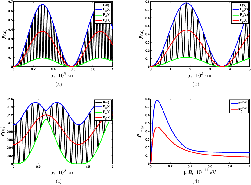
As these plots show, at low matter densities the envelope functions give, at each propagation distance, the range of the possible values of the oscillation probability. At greater matter densities, where the probability oscillates less intensively, the envelope functions are not that useful in analyzing the physical situation.

One can find the maximum value of the upper envelope function, which is also the upper bound for the transition probability, given as

where the value $B^{\prime}$ is the solution of the transcendent algebraic equation, $C_{+{}}C_{-{}}=S_{+{}}S_{-{}}$. The corresponding maximum values of the averaged transition probablility $P_{0}(x)$ are given by

for arbitrary values of $B$. The values of these maxima depend on the size of the quantity $\mu B$. These dependencies are plotted in Figs. 1(d)-3(d). In the case of rapid oscillations the physically relevant quantities, rather than the maxima, are the averaged values of the transition probability, which are also plotted in these figures.

As Figs. 1(d)-3(d) show, the interplay of the matter effect and the magnetic interaction can lead, for a given magnetic moment $\mu$, to an enhanced spin-flavor transition if the magnetic field $B$ has a suitable strength relative to the density of matter $\rho$. In our numerical examples this occurs at $\mu B_{\mathrm{max}}=1.1\times 10^{-12}\thinspace\text{eV}$ for $\rho=10\thinspace\text{g/cc}$, at $\mu B_{\mathrm{max}}=6.6\times 10^{-13}\thinspace\text{eV}$ for $\rho=50\thinspace\text{g/cc}$, and at $\mu B_{\mathrm{max}}=8\times 10^{-13}\thinspace\text{eV}$ for $\rho=100\thinspace\text{g/cc}$. For these values of $\mu B$ both the maxima and the average of the transition probability become considerably larger than for any other values of $\mu B$. Figures 1(b)-3(b) correspond to the situation of maximal enhancement, whereas Figs. 1(a)-3(a) and Figs. 1(c)-3(c) illustrate the situation above and below the optimal strength $B_{\mathrm{max}}$ of the magnetic field.

It is noteworthy that the enhanced transition probability is achieved towards the lower end of the $\mu B$ region where substantial transitions all occur, that is, at relatively moderate magnetic fields. At larger values of $\mu B$ the maximum of the transition probability approaches towards $\cos^{2}(2\theta)$. Indeed, if $\mu B\gg\max(\Phi,V)$, the transition probability can be written in the form (see Ref. [13]) $P(t)=\cos^{2}(2\theta)\sin^{2}(\mu Bt)$. It was found in Ref. [22] that neutrino spin-flavor oscillations can be enhanced in a very strong magnetic field, with the transition probability being practically equal to unity. This phenomenon can be realized only for Dirac neutrinos with small off-diagonal magnetic moments and small mixing angle. As we can see from Figs. 1(d)-3(d) the situation is completely different for big off-diagonal magnetic moments.

One should notice that for long propagation distances consisting of several oscillation periods of the envelope functions, the enhancement effect would diminish considerably due to averaging. In the numerical examples presented in Figs. 1-3 the period of the envelope function is of the order of $10^{3}-10^{4}\thinspace\text{km}$, which is a typical size of a shock wave with the matter densities we have used in the plots (see, e.g., Ref. [23]). Thus the enhanced spin-flavor transition could take place when neutrinos traverse a shock wave.

Let us recall that the above analysis was made by assuming neutrinos to be Dirac particles. We will see below (see Sec. IV) that the corresponding results are quite different in the case of Majorana neutrinos.

We now move to consider Majorana neutrinos, and we shall start by applying our formalism to the ordinary vacuum oscillation of two Majorana neutrinos. The left-handed chirality component of a flavor neutrino $\nu_{\lambda}^{\mathrm{L}}=(1/2)(1-\gamma^{5})\nu_{\lambda}$ is related to the wave functions of Majorana neutrino states through

where $\lambda=\alpha,\beta$ is the flavor index and $\eta_{a}$, $a=1,2$, correspond to a Majorana particle with a definite mass $m_{a}$. In the simplest case the mixing of the flavor states arises purely from Majorana mass terms between the left-handed neutrinos, and then the mixing matrix $U_{\lambda a}$ is a $2\times 2$ and unitary matrix, i.e., $a=1,2$ and, assuming no CP violation, it can be parametrized in the same way as in Eq. (1).

We study the evolution of this system with the following initial condition [see also Eq. (2)]:

where $\mathbf{k}=(0,0,k)$ is the initial momentum and $\nu_{\beta}^{(0)\mathrm{T}}=(0,1)$. The initial state is thus a left-handed neutrino of flavor $\beta$ propagating along the $z$-axis to the positive direction.

As both the left-handed state $\nu_{\lambda}^{\mathrm{L}}$ and Majorana state $\eta_{a}$ have two degrees of freedom, we will describe them in the following by using two-component Weyl spinors. The Weyl spinor of a free Majorana particle obeys the wave equation (see, e.g., [24]),

The general solution of this equation can be presented as [25]

where $E_{a}=\sqrt{m_{a}^{2}+|\mathbf{p}|^{2}}$. The basis spinors $u_{a}^{(\zeta)}$ and $v_{a}^{(\zeta)}$ have the form

where $w_{\pm{}}$ are helicity amplitudes given by [26]

the angles $\phi$ and $\vartheta$ giving the direction of the momentum of the particle, $\mathbf{p}=|\mathbf{p}|(\sin\vartheta\cos\phi,\sin\vartheta\sin\phi,\cos\vartheta)$. The normalization factor $\lambda_{a}$ in Eq. (32) can be chosen as

Let us mention the following properties of the helicity amplitudes $w_{\pm{}}$:

which can be immediately obtained from Eq. (33) and which are useful in deriving the results given below.

The time-independent coefficients $a_{a}^{\pm{}}(\mathbf{p})$ in Eq. (31) have the following form [25]:

where $\eta^{(0)}_{a}(\mathbf{p})$ is the Fourier transform of the initial wave function $\eta_{a}$,

Using Eqs. (31)-(36) we then obtain the following expression for the wave function for the neutrino mass eigenstates:

From Eqs. (35) and (37) it follows that a mass eigenstate particle initially in the left-polarized state $\eta_{a}^{(0)}(\mathbf{r})\sim w_{-{}}(\mathbf{k})e^{\mathrm{i}\mathbf{k}\mathbf{r}}$ is described at later times by