Correlation effects in a discrete quantum random walk

Introduction.— “Random walks” (RWs) is an important and prevalent concept in various branches of science [1], in that many phenomena can be modeled by using the associated notions or tools. A classical random walk (CRW) is the dynamics of a classical (i.e., non-quantum) object — which will be called “particle” or “walker” hereon — within a fully or partially stochastic environment and/or under some stochastic forces. A famous example of such an evolution is encountered in non-equilibrium statistical mechanics of gas particles inside a cylinder. Configuration or state of the walker in a CRW can be described by a local (classically measurable) quantity, such as its “position” (not necessarily real-space position) at each step (or “time”), $x(t)$. A general, and therefore, context-free modeling of a CRW is provided when one can introduce stochasticity/randomness via inclusion of a random object such as a “coin”. A characteristic of a RW is its variance or dispersion, $\sigma^{2}=\langle x(t)^{2}\rangle-\langle x(t)\rangle^{2}$, where $\langle.\rangle$ indicates an ensemble average. For a CRW, this quantity for long times shows a linear behavior with the total walk time: $\sigma^{2}\sim T$, which is a characteristic of a diffusive motion. More generalizations of CRW can be found in literature, for example see Refs. [2, 3, 4, 5, 6, 7] and the references therein.

Recently, there has been a great interest in the dynamics of a quantum random walk (QRW), a quantum object hopping (discretely or continuously) on a graph — e.g., a line — based on an intrinsically quantum mechanical decision-making in each step, e.g., by a quantum coin in a discrete QRW [8, 9, 10, 11, 12, 13, 14, 15, 16, 17]. Moreover, it has been shown that the language of a (continuous) QRW, assisted with suitable Hamiltonian maps, can provide a universal framework for the studies on general qubit systems [18]. One should note that in this type of RWs an external object like a quantum coin is not necessary. In a QRW, the combined dynamics of the coin and the walker is governed by a unitary operation $U_{\text{CW}}$ (acting on $\mathcal{H}_{\text{C}}\otimes\mathcal{H}_{\text{W}}$), which introduces quantum effects such as coherence and entanglement and results in interference between classical paths. This quantum nature is responsible for the features radically different than those of a CRW, such as: a different, spread non-Gaussian probability distribution $P(x,t)$ [12, 16], a quadratically faster spreading $\sigma^{2}\sim T^{2}$ [12, 16, 19, 20] (the ballistic motion), the exponentially faster propagation between particular nodes of a specific graph [11, 13].

Of our special interest in this paper is to numerically investigate how “memory-effects” or “correlations” show up and play a role in the general behavior of a (discrete, coined) QRW. In a RW, the dynamics in every time is generally dictated by the history of the previous step(s) and the coin-flip(s). When the dynamics is Markovian, in principle there is no history in the system, and, the walker’s immediate future is decided only based on its present and an immediate coin-flip [1]. In other words, in a Markovian CRW, by definition, the walker does not keep any memory of its state in previous times. From a physical point of view, it seems that when the walker is interacting with a slowly-responding environment — slow relative to the characteristic time of the walk — it is unlikely that the environment can feed some of the acquired (or leaked) information back to the walker, and therefore, affect its future moves. In this case, the leading effect would be a loss of memory, and accordingly, emergence of a regime in which the Markovian assumption is a valid approximation. As a result, it is expected that in this regime, there would be a negligible correlation between the configurations in distant times. In open quantum systems the analysis of non-Markovian effects is more involved than in the classical case and adding a memory kernel to equations has many complex aspects [21]. Besides, unlike the classical case, in open quantum systems one cannot use the standard approaches like the Chapman-Kolmogorov equation to test the Markovian property [22], because the related joint probabilities might be not well-defined from quantum mechanical perspective. Recently, however, some preliminary progress was reported regarding how to decide whether a quantum channel is Markovian or not [23].

In a discrete QRW, the stepwise coin-walker dynamics, i.e., $|\Psi(t+1)\rangle_{\text{CW}}=U_{\text{CW}}|\Psi(t)\rangle_{\text{CW}}$ for $t\leqslant T$, may imply a Markovian characteristic for the walker’s dynamics as well. Although for the coin-walker system the dynamics is indeed Markovian (or memoryless), this is not generally the case for the walker’s state alone [24]. It has been shown that due to the quantum entanglement between the coin’s and the walker’s states, there can exist a “pseudo” memory (hence non-Markovian effect) in the RW after tracing out over the coin at the last step (or after a few steps). Precisely speaking, in the case of a standard discrete-time QRW with a localized initial state, the quantum probability distribution $P_{\text{quant.}}(x,t)$ is related to all classical probabilities $\{P_{\text{class.}}(x,t^{\prime}):~t^{\prime}\leqslant t\}$ (with the same initial conditions). Tracing over the coin immediately after each step, and averaging over all possible measurement results, generates a CRW [25]. This is typical of systems under decoherence or interaction with an external environment. When the environment observes or measures the system, some coherence, hence dynamical information, would become inaccessible and the system tends to lose its quantum correlations. This has been anticipated as a usual route to manifest classical-like behavior in quantum systems. In the case of a QRW, there are numerous studies specializing on how different sources of decoherence can affect a QRW and induce a transition to a CRW. E.g., tracing over the coin after each step or replacing the used coin with a new one at each step (multiple coins) and tracing over all of them after a while [25, 26, 27], random phase noise on the coin state [15, 28], unitary stochastic noise [29], periodic coin and/or walker measurements or randomly broken links on the graph [30] — for a general review see Ref. [31]. In these studies, the long-time behavior of variance $\sigma^{2}$, for its different scalings for the standard CRW and QRW (as discussed earlier), has been adopted as an indicator to distinguish “classical” and “quantum” regimes of a RW [25]. This approach, although very fruitful, is not necessarily conclusive in that there are quantum diffusion models featuring sub-ballistic, the so-called “anomalous” diffusion, or other types of behaviors [33, 34, 35, 32]. This implies that a deeper characterization of different regimes in quantum systems by other stronger tools is necessary. Moreover, there is still no clear understanding about possible roles memory, correlations, or related environmental effects might play in appearance of different regimes in an open system QRW or transitions between such regimes. A study in this line, therefore, might shed some light and bridge between seemingly different underlying notions and physical behaviors. Here we report a numerical preliminary step that may fill some blanks.

In the following, we introduce a few simple QRW models in which a memory/history-keeping feature is included. First we add a non-Markovian property to a QRW as an uncorrelated mixing of the states at different instants. We show how variance for these models behave vs time, signaling the inadequacy of this quantity for distinguishing different regimes. Next, we consider a more physically motivated model in which, in addition to the coin and the walker, a simple harmonic oscillator has been coupled to play as a history-keeping agent. We define the concepts of correlation and correlation exponent as useful tools for evaluating the effect of memory. The correlation exponent for our model is calculated numerically and contrasted with the exponents of a memory-dependent CRW model [6]. This analysis implies that adding memory may induce anti-correlation similar to what is seen in a self-avoiding CRW.

Uncorrelated history-dependence.— We start by a brief review of the standard (memoryless, discrete) QRW [16]. This model consists of a finite one-dimensional integer lattice forming the walker’s space, $\mathcal{H}_{\text{W}}=\text{span}\{|x\rangle\}_{x=-L}^{L}$, and a chirality (or spin) degree of freedom, $\mathcal{H}_{\text{C}}=\text{span}\{|\pm\rangle\}$, constituting the coin space. The dynamics of $|\Psi(t)\rangle_{\text{CW}}$ is induced by the unitary operator $U_{\text{CW}}(p)=(P_{+}\otimes S+P_{-}\otimes S^{\dagger})(u_{\text{C}}(p)\otimes\openone_{\text{W}})$, where $P_{\pm}$ are projection operators onto $\mathcal{H}_{\text{C}}$, $S=\sum_{x=-L}^{L-1}|x+1\rangle_{\text{W}}\langle x|$ is the shift operator on the graph, and $u_{\text{C}}(p)=\left(\begin{smallmatrix}\sqrt{p}&\sqrt{1-p}\\ \sqrt{1-p}&-\sqrt{p}\end{smallmatrix}\right)$, $0\leqslant p\leqslant 1$, is a unitary quantum coin tossing operator.

Intuitively, one might imagine that a memory-dependent model of a QRW can be built by considering that the state $|\Psi(t+M)\rangle_{\text{CW}}$ is obtained from some operation on a linear combination of the states in the $M$ previous instants: $\{|\Psi(t+m)\rangle_{\text{CW}}\}_{m=0}^{M-1}$. This simple approach is unfortunately doomed to be non-linear hence unphysical, though. There are various ways to avoid non-linearity. Here we consider two simple (though not necessarily physically motivated) models in which the states at different instants are mixed in an uncorrelated and random manner. A rather similar approach has already been used to numerically investigate decoherence effects on a QRW [36].

The first model is based on the density matrices in the $M$ previous steps

Here, $0\leqslant\Gamma_{k}\leqslant 1$ and $\sum_{k}\Gamma_{k}=1$ and $A_{\sigma}^{(k)}$ is the Kraus operator given by $A_{\sigma}^{(k)}=\langle\sigma|U_{\text{CW}}^{k}|C\rangle$, where $|C\rangle=C_{+}|+\rangle+C_{-}|-\rangle$ is the initial state of the coin. Non-Markovian characteristic of this model is apparent for the history-dependence of the walker’s state on its $M$ previous instances. Another feature inferred from Eq. (1) is that in every step we discard the coin, tracing out over it to obtain $\rho_{\text{W}}$, and use a fresh coin prepared as $|C\rangle$ for the next step (multiple coins). Indeed, including multiple coins has already been identified as a way to include history in a QRW [27]. For a balanced initial coin ($C_{+}=-iC_{-}=1/\sqrt{2}$) and a balanced coin-flip ($p=1/2$), if $\Gamma_{1}=1$ we obtain a behavior similar to an unbiased memoryless CRW in the sense of variance (see Fig. 1). Degree of history-dependence of the model is adjusted by $\Gamma_{k}$s. For numerical simulations, in addition to the aforementioned conditions, we have taken $M=2$ and $T=100$, with the walker initially localized at the origin. Figure 2 depicts the peaks of the probability distribution $P(x,100)$ for varying $\Gamma$. Notice that for a range of values of $\Gamma$, the probability distribution exhibits a bimodal behavior, similar to a memoryless QRW. As $\Gamma$ increases, the the peaks approach each other and eventually merge into one for $\Gamma\approx 0.8$. As indicated in the inset of Fig. 1, for this walk a $\sigma^{2}\sim a(\Gamma)t^{2}+b(\Gamma)t+c(\Gamma)$ fitting can be found for different values of $\Gamma$ — with $\sigma^{2}\sim t$ for $\Gamma=1$. In this respect this model shows characteristics of both QRW and CRW for different ranges of $\Gamma$.

The second model is an uncorrelated mixing of some unitary dynamics which overall constitutes a dependence on information from the $M$ previous steps. Using $M$ different quantum coin-walk operators, $U_{\text{CW}}(p_{k})\equiv U_{\text{CW}}^{(k)}$ (for notational convenience), generated by $\{p_{k}\}_{k=1}^{M}$, the evolution is described as the following:

Again, $0\leqslant\Gamma_{k}\leqslant 1$ and $\sum_{k}\Gamma_{k}=1$. The density matrix at each time $t>1$ will involve some mixing of the different coins-walks, introducing correlations. If $M=1$ or $\Gamma_{1}=1$, this reduces to the memoryless QRW. Like Eq. (1), the degree of correlations can be adjusted by $\Gamma_{k}$. However, unlike the previous model, there is no bifurcation or transition from bimodality to unimodality in the behavior of the probability distribution vs $\Gamma$ — see Fig. 3.

A simple harmonic oscillator model.— A more physically relevant picture in which the roles of correlations and memory-dependence may be explained is through the Hamiltonian formalism. To this end, keeping the discussion simple (for numerics), we modify the “Hamiltonian” of the memoryless coined QRW model so that a history-keeping agent can be added. This picture can easily be generalized to more realistic cases in which the dynamics is continuous in time and also there is no need for an extra quantum coin. The Hamiltonian of the memoryless QRW can be found from $U_{\text{CW}}(p)=e^{i\frac{\pi}{2}}e^{iZ\otimes P}e^{-i\frac{\pi}{2}(\sqrt{1-p}X+\sqrt{p}Z)}$ by using the Baker-Campbell-Hausdorff formula. Now consider that the walker is coupled to a simple harmonic oscillator and a reservoir consisting of a sufficiently large number of excitation modes in the following manner:

Although this “Hamiltonian” models a crude simplification, clearly lacking various realistic characteristics, to some extent it has been inspired by a cavity QED-based proposal for a QRW  [37], and serves well enough for demonstration of our ideas. In Eq. (3), $H_{\text{O}}=\frac{1}{2}\omega a^{{\dagger}}a$, $H_{\text{R}}=\frac{1}{2}\sum_{k=1}^{\infty}\Omega_{k}c_{k}^{{\dagger}}c_{k}$, and for the coupling of the oscillator and reservoir degrees of freedom we can take, for example, $H_{\text{OR}}=g(a\sum_{k=1}^{\infty}c_{k}^{{\dagger}}+a^{{\dagger}}\sum_{k=1}^{\infty}c_{k})$, where $a$ is the lowering operator of the oscillator ($a^{{\dagger}}a|n\rangle_{\text{O}}=n|n\rangle_{\text{O}}$, for $0\leqslant n\leqslant n_{\max}<\infty$) and $c_{k}$ is the annihilation operator of the $k$th excitation mode. The walker-oscillator coupling term, $H_{\text{WO}}=\lambda P(a+a^{{\dagger}})$, implies that as the walker moves over the lattice, energy is being exchanged with the oscillator, and the oscillator gets partial information about the walker. This interaction is effectively a momentum-position coupling, which preserves the walker’s momentum. The history-dependence in this model is modulated by the coupling constant $\lambda$ ($\lambda=0$ corresponds to the memoryless QRW). The coefficient $g$, instead, controls the effect of the reservoir. The mediated coupling of the oscillator to the reservoir may also result in long-term correlations — this, however, needs a closer analysis which is beyond the scope of this paper. Considering that $[H_{\text{CW}},H_{\text{WO}}+H_{\text{O}}]=0$, we have $U_{\text{CWO}}=U_{\text{CW}}e^{-i(H_{\text{WO}}+H_{\text{O}})}$. To maintain tractability of the numerical simulations, here we make the following assumptions: (i) ignoring the reservoir effect, i.e., $g=0$, (ii) taking a balanced coin-flip ($p=1/2$) and an initially balanced coin, (iii) the walker is initially localized at the center, (iv) $\omega=5$, (v) $T=60$, (vi) periodic boundary condition, $S|L\rangle_{\text{W}}=|-L\rangle_{\text{W}}$, with $L=75$, (vii) the oscillator is initially prepared at the ground state $|0\rangle_{\text{O}}$, (viii) the oscillator energy levels (or Hilbert space) are truncated at $n_{\max}=10$, and (ix) working in $0\leqslant\lambda\leqslant 1$ interval for the coupling constant. Validity of assumption (viii) is confirmed through the simulations noting that after $T=60$ the maximum probability for $|10\rangle_{\text{O}}$ being populated is of the order of $10^{-24}$. Moreover, we have seen that taking $L=75$ and $T=60$ makes the boundary effects insignificant.

Figure 4 depicts the probability distribution for the modified QRW model at $T=60$, in which symmetry is accounted for by the symmetry of the initial conditions. The distribution with $\lambda=0.1$ maintains a relatively similar behavior as the memoryless QRW — indicating a weak coupling regime — whilst there are non-zero probabilities everywhere on the lattice due to the $\lambda$-coupling, indicating spreading of the distribution as compared to the memoryless QRW. This can can be seen in Fig. 5, variance vs time for three different values of $\lambda$, in which a fitting of the form $a(\lambda)t^{2}+b(\lambda)t+c(\lambda)$ yields $a(1)\approx 2.519$, $a(0.1)\approx 0.295$, and $a(0)\approx 0.292$ — a faster spreading for the modified model, which may be understood by noting that the $\lambda$-coupling favors hopping of the walker.

Comparison of the walks.— To make a meaningful comparative analysis of how memory and correlations behave in different RWs, we choose a memory-dependent CRW model proposed in Ref. [6] (for other memory-dependent CRW models see, for example, [2, 3, 4, 7]). This model is interesting in that it features various aspects of a real-world history-keeping systems, such as “saturation” of memory (i.e., finite memory capacity). Unfortunately a direct quantum mechanical extension of the model entails non-linearity and necessity of feedback. In this model, memory is based on the “information” of the sites, which is determined by the number of the times the walker visits each site as well as the times in which these visits occur. The walker hops from site $i$ to a neighboring site $j$ with the probability $p_{ij}\sim e^{u(s_{j}-s_{i})}$, where $s_{i}(t)=\sum_{m}n_{i}(m)e^{-\kappa(t-m)}$ is the remaining information at site $i$ at time $t$. Here $u$ is the density of information energy; $u>0$ ($u<0$) corresponds to a walker attracted to (repelled by) sites with high information content and $u=0$ gives the memoryless CRW. The coefficient $\kappa\geqslant 0$ is the memory decay exponent, for our simulations fixed at $\kappa=10^{-4}$, and $n_{i}(m)$ is $1$ if site $i$ was visited at time $m$ and $0$ otherwise. A saturated information amount, $s_{\max}$, is assumed above which the effect of information ceases to increase ($s(t)\leqslant s_{\max}$), which for our simulations is taken to be $13$. The effect of memory on the scaling exponents of the RW, in terms of the number of sites visited and the distance the walker travels from its initial position, has been examined [6], demonstrating that for any $\kappa>0$ and finite $u$ this RW exhibits a similar scaling behavior of variance to that of a memoryless CRW. As $u\rightarrow\infty$, the scaling behavior of the variance of this model changes from $\sigma^{2}\sim T$ to $\sigma^{2}\sim c$, where $c$ is a constant; whilst for $u\rightarrow-\infty$, the scaling changes from $\sigma^{2}\sim T$ to $\sigma^{2}\sim T^{2}$. For our numerical analysis $u$ remains restricted such that the variance behaves as expected for CRW. The probability distribution for this memory-dependent CRW is calculated using $10^{4}$ independent repetitions and an averaging over the results.

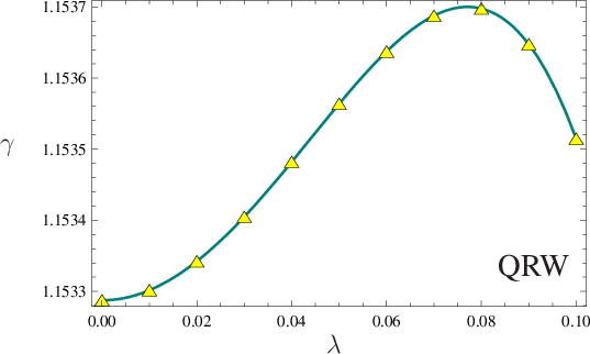
A standard method to characterize short- and/or long-term memory-dependent behaviors in data analysis is through calculation of (auto-) correlation functions [38]. In the case of quantum diffusion systems, it has also been argued that the temporal scaling behavior of the correlation function can show some universal characteristic relation with the spreading and the spectrum [39, 33, 40, 34, 35, 41]. We adopt a modified definition for the correlation function as follows. From the probabilities at a fixed $x^{*}$ for varying time $t$ (up to $T\lesssim\infty$), the time-series $\{P_{x^{*}}(t)\}_{t=0}^{T}$ is generated. Next, we define $C_{x^{*}}(\tau)\equiv\sum_{t=0}^{T-\tau}P_{x^{*}}(t)P_{x^{*}}(t+\tau)$. An advantage of this definition, to the one used in Refs. [39, 33, 40, 34], is that ours allows to build time-series data for a QRW in the same footing as CRW. Besides, it enables application of (classical) data analysis tools, e.g., detrended fluctuation analysis [42], for finding trends and fractal behaviors in a data set. It has been shown that the correlation function exhibits a power-law (i.e., algebraic) decay as $C(\tau)\sim\tau^{-\gamma}$, where $\gamma$ — the correlation exponent — is related to spectral properties of the system [33]. A small value of $\gamma$ is an attribute of a walk that stays relatively localized, whilst a large $\gamma$ indicates a tendency for the walker’s distribution to spread with time. The correlation function has been calculated for the memory-dependent CRW (for $u=\{0,\pm 0.1\}$) and the modified QRW (for $\lambda=\{0,0.01,0.1\}$) at $x^{*}=0$. The value of $C(\tau)$ is very small for odd values of $\tau$. This is because the probability of the walker occupying the origin in odd $t$s is small. These probabilities are non-zero in the case of $\lambda>0$ as seen earlier. In CRW and for $\lambda=0$, this probability is zero. The even (time) points of the correlation function have been fitted to $C(\tau)\sim a+b\tau^{-\gamma}$ — Fig. 6 — with $\gamma_{\text{QRW}}\approx 1.153$, $\gamma_{\text{SAv-CRW}}\approx 0.01$, $\gamma_{\text{CRW}}\approx 0.005$, and $\gamma_{\text{SAt-CRW}}\approx 0.003$. The behavior of $\gamma$ vs $\lambda$ has been plotted in Fig. 7. A preliminary analysis suggests that the peak in this plot may be a byproduct of the finite size of the system. A closer investigation, however, may suggest a better explanation for possible underlying reason(s). The property $\gamma_{u=0.1}<\gamma_{u=0}<\gamma_{u=-0.1}$ is in accordance with our understanding about the physical meanings of positive and negative $u$s, i.e., self-attracting and self-avoiding, respectively. An interesting observation is that in the limit of $u\rightarrow-\infty$, SAv-CRW and QRW show similar general behaviors.

Summary.— We have introduced simple quantum random walk models with memory-dependent features by adding a non-Markovian property to the walk as an uncorrelated mixing of the states at different instants and also by introducing a Hamiltonian picture with a memory modulating coupling. Variance vs time for the uncorrelated models has been calculated. In the Hamiltonian model, we have defined and calculated the concepts of correlation and correlation exponent as useful tools for assessing the effect of memory or correlation. Comparison with classical memoryless and memory-dependent models has indicated an anti-correlation in the quantum random walk. Variance as an indicator to distinguish between classical and quantum regimes has apperared to be a not so useful tool. We, instead, have suggested that tools such as correlation exponents and detrended fluctuation analysis are probably more useful in characterizing different regimes of a quantum system. These studies may shed some light on how different regimes of behaviors in quantum diffusion systems emerge and how they are related to other physical characteristics of those systems. Also, these might have some implications on when a quantum random walk based algorithm for a problem may result in a speedup in comparison to classical algorithms.

Acknowledgements.— This work was supported by CIFAR, iCORE, MITACS, NSERC, and PIMS.

References

- [1] N. G. van Kampen, Stochastic Processes in Physics and Chemistry (North Holland, Amsterdam, 2001); H. C. Berg, Random Walks in Biology (Princeton University Press, Princeton, 1993); R. N. Mantegna and H. E. Stanley, An Introduction to Econophysics: Correlations and Complexity in Finance (Cambridge University Press, Cambridge, UK, 2000); R. Motwani, and P. Raghavan, Randomized Algorithms (Cambridge University Press, Cambridge, UK, 1995).
- [2] H. Hara, Phys. Rev. B 20, 4062 (1979).
- [3] H. E. Stanley et al., Phys. Rev. Lett. 51, 1223 (1983).
- [4] R. Hilfer, Phys. Rev. B 44, 638 (1991).
- [5] A. Ordemann et al., Phys. Rev. E 61, R1005 (2000).
- [6] Z. -J. Tan et al., Phys. Rev. E 65, 041101 (2002).
- [7] U. Keshet and S. Hod, Phys. Rev. E 72, 046144 (2005).
- [8] Y. Aharonov, L. Davidovich, and N. Zagury, Phys. Rev. A 48, 1687 (1993).
- [9] D. A Meyer, J. Stat. Phys. 85, 551 (1996).
- [10] J. Watrous, J. Comput. Sys. Sci. 62, 376 (2001).
- [11] E. Farhi and S. Gutmann, Phys Rev. A 58, 915 (1998).
- [12] A. Nayak and A. Vishwanath, eprint quant-ph/0010117 (2000).
- [13] A. M. Childs et al., in Proceedings of the 35th ACM Symposium on Theory of Computing (STOC 2003), San Diego, CA (ACM Press, New York, 2003), p. 59.
- [14] A. M. Childs and J. Goldstone, Phys. Rev. A 70, 022314 (2004).
- [15] T. D. Mackay et al., J. Phys. A: Math. Gen. 35, 2745 (2002).
- [16] J. Kempe, Contemp. Phys. 44, 307 (2003).
- [17] F. W. Strauch, Phys. Rev. A 74, 030301(R) (2006).
- [18] A. P. Hines and P. C. E. Stamp, Phys. Rev. A 75, 062321 (2007).
- [19] A. Romanelli et al., Phys. Lett. A 313, 325 (2003).
- [20] A. Romanelli et al., Physica A 338, 395 (2004).
- [21] H. -P. Breuer, Phys. Rev. A 70, 012106 (2004); H. -P. Breuer, J. Gemmer, and M. Michel, Phys. Rev. E 73, 016139 (2006); S. Maniscalco and F. Petruccione, Phys. Rev. A 73, 012111 (2006); A. A. Budini, Phys. Rev. A 69, 042107 (2004); A. Shabani and D. A. Lidar, Phys. Rev. A 71, 020101(R) (2005).
- [22] R. Friedrich, J. Peinke, and Ch. Renner, Phys. Rev. Lett. 84, 5224 (2000).
- [23] M. M. Wolf, J. Eisert, T. S. Cubitt, and J. I. Cirac, e-print: arXiv:0711.3172.
- [24] A. J. Bracken, D. Ellinas, and I. Tsohantjis, J. Phys. A: Math. Gen. 37, L91 (2004).
- [25] T. A. Brun, H. A. Carteret, and A. Ambainis, Phys. Rev. Lett. 91, 130602 (2003).
- [26] T. A. Brun, H. A. Carteret, and A. Ambainis, Phys. Rev. A 67, 052317 (2003).
- [27] A. P. Flitney, D. Abbott, and N. F. Johnson, J. Phys. A: Math. Gen. 37, 7581 (2004).
- [28] J. Košik, V. Bužek, and M. Hillery, Phys. Rev. A 74, 022310 (2006).
- [29] D. Shapira et al., Phys. Rev. A 68, 062315 (2003).
- [30] A. Romanelli et al., Physica A 347, 137 (2005).
- [31] V. Kendon, Math. Struct. Comput. Sci. 17, 1169 (2007).
- [32] N. V. Prokof’ev and P. C. E. Stamp, Phys. Rev. A 74, 020102(R) (2006).
- [33] J. X. Zhong and R. Mosseri, J. Phys.: Condens. Matter 7, 8383 (1995).
- [34] J. X. Zhong et al., Phys. Rev. Lett. 86, 2485 (2001).
- [35] S. Mukhopadhyay, M. Saglam, and Chatterjee, Eur. Phys. J. B 59, 69 (2007).
- [36] O. Maloyer and V. Kendon, New J. Phys. 9, 87 (2007).
- [37] B. C. Sanders et al., Phys. Rev. A 67, 042305 (2003).
- [38] J. Honerkamp, Statistical Physics: An Advanced Approach with Applications (Springer-Verlag, Berlin, 2002).
- [39] R. Ketzmerick, G. Petschel, and T. Geisel, Phys. Rev. Lett. 69, 695 (1992).
- [40] R. Ketzmerick, K. Kruse, S. Kraut, and T. Giesel, Phys. Rev. Lett. 79, 1959 (1997).
- [41] P. Ribeiro, P. Milman, and R. Mosseri, Phys. Rev. Lett. 93, 190503 (2004).
- [42] K. Hu et al., Phys. Rev. E 64, 011114 (2001).