Low-frequency excitation of double quantum dots
Abstract
We address theoretically adiabatic regime of charge transport for a model of two tunnel-coupled quantum dots connected in series. The energy levels of the two dots are harmonically modulated by an external potential with a constant phase shift between the two. Motivated by recent experiments with surface-acoustic-wave excitation, we consider two situations: (a) pure pumping in the absence of external voltage (also at finite temperature), and (b) adiabatic modulation of the current driven by large external bias. In both cases we derive results consistent with published experimental data. For the case (b) we explicitly derive the adiabatic limit of Tien-Gordon formula for photon-assisted tunneling and compare it to the outcome of simple conductance modulation. A tutorial for adiabatic pumping current calculations with the Green function formalism is included.
keywords
quantum dots, adiabatic transport, pumping, double dots, surface acoustic waves1 INTRODUCTION
Alternating external fields applied locally to a confined electronic structure can result in a measurable time-averaged current across the device. Generating dc current by microwave excitation at frequencies of several GHz and less is often referred to as pumping. Particular appeal of pumping both as a research tool and a potential source of applications for nanoelectronic systems is that low-frequency fields can be confined to wave-guides and wires and thus conveniently delivered to samples at a few Kelvin or lower temperatures. This opens the way to explore pumping in situations when quantum coherence and single-electron charging effects matter.
Particular motivation for this work has been provided by two recent experiments [1, 2] in which electrons in quantum dots have been subjected to an alternating piezoelectric potential of a running surface acoustic wave (SAW). The experiment of Buitelaar et al.[1] focused on pure pumping current with no external dc voltage bias. Experimental results have been reported to be in a good agreement with the theory of adiabatic quantum pumping[3] applied to a simple two-level model (see definition and discussion in Secs. 2 and 3 of the present paper). The experiment of Naber et al.[2] has been designed to measure the influence of an oscillating SAW potential on directed current driven by a constant external voltage but not necessarily by the SAW-induced potential itself. The results were found to be in a good agreement with Tien-Gordon formula[4, 5] of photon-assisted tunneling.
In this paper we show that the results of these two experiments are consistent within one and the same model: in the large bias limit, adiabatic conductance modulation for the two-level system of Ref. [1] reproduces the major features of the current traces reported in Ref. [2] (except for the fine structure due to non-adiabaticity). We derive analytically the adiabatic limit of Tien-Gordon formula and reproduce the criterion[6] for the validity of an adiabatic approximation: inverse life-time of the discrete charge states, , must be larger than the modulation frequency .
This paper has two major components. After introducing the model in Sec. 2, we discuss in detail the adiabatic pumping current and its various limits (Sec. 3). These results have been used directly for interpretation of experimental data on pumping in carbon nanotube quantum dots[1]. The discussion in Secs. 2 and 3 is more of a tutorial style. In the second part of the paper, Sec. 4, we turn to the limit of large bias in which adiabatic conductance modulation dominates over pure pumping. We compare predictions of the adiabatic time-domain expansion [7] (essentially, time-average of the Landauer formula) to the low-frequency limit of the photon-assisted tunneling through a double dot [4, 5]. This comparison uncovers precise agreement between the two theories (up to an overall integer factor) and establishes a rigorous adiabaticity criterion. Comparison to the experimental data of Naber et al identifies the adiabatic features in the measured current line-shape. A brief summary and an outlook at open challenges in Sec. 5 concludes the paper.
2 THE MODEL AND ITS STATIC PROPERTIES
The Hamiltonian describes two energy levels, and , with off-diagonal tunneling coupling , connected to two external reservoirs: level to the left (), level to the right (). In the second quantized form,
| (1) |
The boundary conditions imposed onto are those of equilibrium reservoirs at electrochemical potentials and (for the left and the right lead correspondingly) and at equal temperatures . The difference specifies the external dc bias, while the average sets the reference level for energy.
We shall take in Eq. (1) to be independent of energy (the limit of a structureless, wide band ). In this case the only parameter characterizing the leads is the golden rule half-width . If no lead index is specified, the couplings will be assumed symmetric, . When discussing near-equillibrium properties (linear conductance, abiabatic pumping) we shall assume vanishing bias conditions, .
The reason we omit physical spin index in Eq. (1) is that the dots are assumed to be in the Coulomb blockade regime, so that double occupancy of a single dot in energetically prohibited. This assumptions of “spinless & non-interacting” electrons can be viewed as a fermionic representation of the charge state transition in an otherwise inert (that is, devoid of any internal dynamics) Coulomb-blockaded quantum dot. For a single dot this representation results in the well-known single resonant level (Breit-Wigner) approximation to Coulomb blockade [8]. Applicability of a non-interacting Hamiltonian like (1) to a pair of tunnel-coupled quantum dots is thoroughly discussed in Sec. V of a review[9] by van der Wiel et al. While incomplete in its treatment of mutual capacitance and correlation effects, the non-interacting charge-carrier approach adopted here allows for a very detailed investigation of time-dependent effects because of the its fundamentally single-particle nature.
Some aspects of non-adiabatic pumping for the system defined by Eq. (1) have been considered recently [10] using a Floquet formulation for time-periodic non-equilibrium Green functions. Our model is also a special (and previously unexplored) case of the a tight-binding model for SAW-induced adiabatic pumping as introduced and studied in Ref. [11, 12]11 1 In the notation of Ref. [12], one has to consider , take the limit of with and identify with ..
It is convenient[13] to define the retarded Green function matrix, , for the double-dot region in the following way[14],
| (2) | |||
| (3) |
The transmission probability from left to right[14],
| (4) |
determines the linear conductance via (the finite-temperature) Landauer formula, . Here and below is the Fermi distribution function.
For our system the transmission probability is [see Eqs. (2) and (4)]
| (5) |
were the denominator is given explicitly by
| (6) | ||||
| (7) |
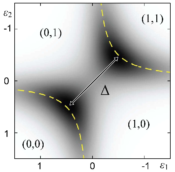
The eigenenergies and , can be understood as “molecular orbital” states of the double dot system. For the resonance lines of are resolved in a two-dimensional plot of as a function of and , see Fig. 1. Such diagrams are often referred to as stability diagrams[9] for systems of coupled quantum dots since they identify the regions of different equilibrium occupation numbers for the dots. Anti-crossing behavior seen in Fig. 1 is a hallmark of a tunnel-coupled double dot system and serves as a conceptual basis for charge-qubit approaches to quantum information processing [15].
.
3 ADIABATIC PUMPING
We envision pumping by modulating and with the help of a piezoelectric potential of a propagating SAW (or, perhaps, by direct gating). This requires calculating the response of the system to time-variation of the double-dot parameters22 2 For simplicity, the effect of the modulating field on the tunnel couplings is assumed to be negligible.. One of the simplest scenarios [1] is a phase-shifted harmonic modulation:
| (8) | ||||
| (9) |
where is a constant detuning between the levels and is the amplitude of the external potential. However, in this section we shall focus on general properties of the adiabatic pumping current which are independent of a particular choice of .
Let us apply the general theory of adiabatic transport in coherent strctures[7] to Hamiltonian (1) using a Green function formalism[13]. Instantaneous adiabatic current entering lead from the nanostructure is[13]
| (10) |
The charge pumped by the system during one cycle of the periodic modulation with a circular frequency is
| (11) |
where
| (12) | ||||
| (13) |
Since we have used a symmetrized current expression in Eq. (11), under .
As usual for two-parameter pumps[3], it is convenient for the subsequent analysis to transform the contour integral in Eq. (11) into an surface integral using Green’s theorem. We write as a double integral over the area enclosed by the contour:
| (14) |
Volume under the two-dimensional plot of above the pumping contour’s image in the plane gives the value . The sign of is determined by the direction of the contour [plus in Eq. (14) for counterclockwise direction]. This way of visualizing the pumping response is illustrated in Fig. 2.

Restricting the discussion to allows for some further analytical progress. Performing the integration over the energy , we obtain explicitly
| (15) |
where and is the digamma function.
Let us consider also the maximal possible charge per period () which is obtained when a large pumping contour completely encompasses the positive part of . For an arbitrary ratio we find:
| (16) |
Specific limits of and are illustrated below.


3.1 Tunneling-dominated limit:
The function for simplifies to
| (17) |
The maximal possible charge (16) becomes
| (18) |
This is illustrated in the left panel of Fig. 3. We see that charge quantization (meaning ) is possible when . In this limit the two resonance lines in Fig. 1 are well-defined, and pumped charge quantization proceeds via the loading-unloading mechanism[13].
3.2 Temperature-dominated limit:
In the opposite extreme of temperature-broadened resonance lines we have
| (19) |
(prime denotes energy derivative). The corresponding maximal charge is
| (20) |
This limit of the model approximates the conditions of the seminal experimental work of Pothier et al.[16]. Note that the “exponential” accuracy is possible only as long as so that co-tunneling and other higher-order processes remain below the level of thermal fluctuations.
4 CONDUCTANCE MODULATION AT LARGE BIAS
4.1 Adiabatic pumping in the presence of external dc bias
Let us turn to a situation when a constant bias voltage is applied together with a slow modulation of the system parameters. General formalism for this scenario has been considered in Ref. [7]. The instantaneous adiabatic current from left to right has been found to contain two additional components on top of the pure pumping contribution (10):
| (21) |
In our notation, the results of Entin-Wohlman et al.[7] for the time-average current read
| (22) | ||||
| (23) |
Here is the overall transmission (Friedel) phase[17].
Interpretation of Eq. (22) is straight-forward[7] — it is the time-average of the current given by the finite-bias Landauer formula. Adiabatic perturbation of the system manifests itself in Eq. (22) only as a parametric modulation of the transmission function . The last remaining term, Eq. (23), is harder to interpret. It is non-zero only if both the bias and the adiabatic modulation are present at the same time (thus the notation ).
We observe that both [Eq. (10)] and [Eq. (23)] contain the Fermi functions only in the form of the respective energy derivatives. If and the bias window is sufficiently wide to cover the whole energy range where the transmission function is appreciable, then the conductance-modulation term, , dominates in the total current (21). In the remaining part of this section we are going to explore the large bias limit for the model defined in Eq. (1) and subjected to a harmonic modulation (8) and (9).
4.2 Large-bias current through a modulated double-dot system
The average dc current in the large bias limit, , is
| (24) |
To derive the above equation we have performed the energy integration in Eq. (22) using Eq. (4) and extending the bias window to . The result for the time-averaged directed current (24) is of the form
| (25) |
with and some positive constant . Thus the comparison to an experiment can be made without the detailed knowledge of the tunnel couplings. Only the three scale factors — for the current , the detuning and the modulation amplitude — have to be adjusted. We compare Eq. (25) with the experimental results of Naber et al in Fig. 4.

Our result quantifies the qualitative adiabatic arguments of Naber et al. concerning the increased time at resonance near the turning points of harmonic modulation[2].
4.3 Comparison to the non-adiabatic theory of Stoof and Nazarov
Large bias limit for transport through two capacitatively coupled quantum dots connected in series has been considered theoretically by Stoof and Nazarov[5]. In the limit of a very weak inter-dot tunneling, , zero temperature and strong asymmetry , , they find the following expression for the time-average current33 3 This is equation (21) of Ref. [5] in our notation.
| (26) |
Here is the -th order Bessel function of the first kind. A similar formula is known from the theory of photon-assisted tunneling between two superconductors due to Tien and Gorgon[4], therefore Eq. (26) is sometimes referred to by their name[9]. It has been successfully applied to several experiments on microwave excitation of double quantum dots[9], as well as to the measurements of Naber et al.[2] that we used in Fig. 4.

We would like to compare Eq. (25) to limit of Eq. (26). This limit is singular and requires some care in implementation. To this end, we note that Eq. (26) represents a convolution of the Bessel function with a Lorentzian, see Fig. 5. Typical width of this Lorentzian along a (dimensionless) -axis is while the period of oscillations of is of order one. Evidently, in the limit the fine oscillatory structure of the current as a function of will be washed out. This is the validity condition for the adiabatic limit to Eq. (26) that we are in a position to derive.
The Bessel function oscillates for as 44 4 The highly accurate approximation (27) is derived by taking and applying the stationary phase expansion in to an integral representation of the Bessel function, .
| (27) |
Equation (27) contains the analytic form for the envelope of oscillations shown in Fig. 5. Replacing the sum in Eq. (26) with an integral, using Eq. (27) and dropping the rapidly oscillating term gives
| (28) |
By derivation, Eq. (28) approximates well the full non-adiabatic result (26) if .
If we now expand the adiabatic result (24) to the leading order in and take the limit then Eq. (28) is recovered up to a factor of 4,
| (29) |
To a reasonable degree of confidence we have excluded the possibility that the factor of four arises due a notational or/and algebraic mistake. Of course, we should bare in mind that the Hamiltonian of Stoof and Nazarov is different form ours: they consider the case of both strong intra-dot and inter-dot Coulomb repulsion. Only three states of an isolated double dot system are possible in their case while in ours there is the forth state — the doubly occupied configuration .
5 CONCLUSIONS
Steady progress in experimental manipulation of nanoscale systems such as quantum dots and wires has recently reached a level enabling direct comparison between theory and experiment for pumping in these devices. Many observed features of the pumping currents can be explained within a framework of single-electron models with time-dependent energy levels. In this paper we have looked at two examples of application for this framework to recent experiments. It is quite satisfactory to find agreement between different limits of different devices that comes within a single model. It is conceivable that in the future more refined experiments will allow for quantitative characterization of the pumping current magnitude beyond the accuracy of a simple single-electron picture. Clear separation between the effects of discrete charging, quantum interference and many-body correlations in pumping through nanostructure seems posees future challenges both for theory and experiment.
Acknowledgements.
The author is thankful to Bernd Kästner and Mark Buitelaar for continuous stimulating discussions on the subject. This research has been supported by the European Social Fund (agreement no. 2004/0001/VPD1/ESF/PIAA/04/NP/3.2.3.1/0001/0001/0063).References
- [1] Buitelaar, M. R., Kashcheyevs, V., Leek, P. J., Talyanskii, V. I., Smith, C. G., Anderson, D., Jones, G. A. C., Wei, J., and Cobden, D. H., “Adiabatic charge pumping in carbon nanotube quantum dots,” e-print arXiv:0804.3219, accepted for publication in Phys. Rev. Lett. (2008).
- [2] Naber, W. J. M., Fujisawa, T., Liu, H. W., and van der Wiel, W. G., “Surface-acoustic-wave-induced transport in a double quantum dot,” Phys. Rev. Lett. 96(13), 136807 (2006).
- [3] Brouwer, P. W., “Scattering approach to parametric pumping,” Phys. Rev. B 58(16), R10135 (1998).
- [4] Tien, P. K. and Gordon, J. P., “Multiphoton process observed in the interaction of microwave fields with the tunneling between superconductor films,” Phys. Rev. 129, 647 (1963).
- [5] Stoof, T. H. and Nazarov, Y. V., “Time-dependent resonant tunneling via two discrete states,” Phys. Rev. B 53(3), 1050 (1996).
- [6] Moskalets, M. and Büttiker, M., “Floquet scattering theory of quantum pumps,” Phys. Rev. B 66, 205320 (2002).
- [7] Entin-Wohlman, O., Aharony, A., and Levinson, Y., “Adiabatic transport in nanostructures,” Phys. Rev. B 65, 195411 (Apr 2002).
- [8] Alhassid, Y., “The statistical theory of quantum dots,” Rev. Mod. Phys. 72, 895 (2000).
- [9] van der Wiel, W. G., Franceschi, S. D., Elzerman, J. M., Fujisawa, T., Tarucha, S., and Kouwenhoven, L. P., “Electron transport through double quantum dots,” Reviews of Modern Physics 75(1), 1 (2003).
- [10] Strass, M., Haänggi, P., and Kohler, S., “Nonadiabatic electron pumping: Maximal current with minimal noise,” Physical Review Letters 95(13), 130601 (2005).
- [11] Aharony, A. and Entin-Wohlman, O., “Quantized pumped charge due to surface acoustic waves in a one-dimensional channel,” Phys. Rev. B 65, 241401 (2002).
- [12] Kashcheyevs, V., Aharony, A., and Entin-Wohlman, O., “Quantized charge pumping by surface acoustic waves in ballistic quasi-1d channels,” Eur. Phys. J. B 39, 385 (2004).
- [13] Kashcheyevs, V., Aharony, A., and Entin-Wohlman, O., “Resonance approximation and charge loading and unloading in adiabatic quantum pumping,” Phys. Rev. B 69, 195301 (2004).
- [14] Datta, S., [Electronic transport in mesoscopic systems ], Cambridge University Press, Cambridge (1997).
- [15] Fujisawa, T., Hayashi, T., Jung, S. W., Jeong, Y.-H., and Hirayama, Y., [Quantum Computing in Solid State Systems ], ch. Single-electron charge qubit in a double quantum dot, 279–287, Springer, New York (2006).
- [16] Pothier, H., Lafarge, P., Urbina, C., Esteve, D., and Devoret, M. H., “Single-electron pump based on charging effects,” Europhys. Lett. 17, 249 (1992).
- [17] Langreth, D. C., “Friedel sum rule for Anderson’s model of localized impurity states,” Phys. Rev. 150, 516 (1966).