跳到论文正文
W Papers独立论文阅读器 arXiv:0809.0783 论文正文 计算阅读时间 · 0%
引用这篇论文根据当前论文元数据生成,正式投稿前建议核对。


License: arXiv.org perpetual non-exclusive license
arXiv:0809.0783v2 [hep-th] 22 Jan 2009

The Bethe Ansatz for AdS5×S5{\rm AdS}_{5}\times{\rm S}^{5} Bound States

Preprint:  ITP-UU-08-52
SPIN-08-42
Marius de Leeuw Note: E-mail: M.deLeeuw@uu.nl Affiliation: Institute for Theoretical Physics and Spinoza Institute,
Utrecht University, 3508 TD Utrecht, The Netherlands
Abstract: 

We reformulate the nested coordinate Bethe ansatz in terms of coproducts of Yangian symmetry generators. This allows us to derive the nested Bethe equations for arbitrary bound state string S-matrices. The bound state number dependence in the Bethe equations appears through the parameters x±x^{\pm} and the dressing phase only.

1 Introduction and summary

The AdS/CFT correspondence [1] has been the subject of intensive research. This duality provides a powerful tool to study a plethora of interesting topics in theoretical physics. One of the best studied examples is 𝒩=4\mathcal{N}=4 SYM gauge theory which is conjectured to be dual to superstring theory on AdS5×S5{\rm AdS}_{5}\times{\rm S}^{5}. However, even testing or proving the duality for these concrete models is a difficult problem.

A breakthrough in the understanding of this duality was the discovery of integrable structures. Integrability was found in 𝒩=4\mathcal{N}=4 super Yang-Mills theory by the appearance of (integrable) spin chains describing the operator spectrum [2]. The classical string sigma model on AdS5×S5{\rm AdS}_{5}\times{\rm S}^{5} was also shown to be integrable [3]. If the full quantum theories also exhibit integrable structures, then that would constrain them considerably. For example, in scattering processes for integrable theories the set of particle momenta is conserved and scattering processes always factorize into a sequence of two-body interactions. This implies that in such theories the scattering information is encoded in the two-body S-matrix. Unfortunately, a full proof of integrability of both theories is currently still lacking, but nevertheless there is a lot of evidence hinting that integrability is a feature of the full quantum theories.

By assuming integrability one can make use of the S-matrix approach. This proved to be a powerful instrument to study the operator spectrum of 𝒩=4\mathcal{N}=4 SYM. [2, 4, 5, 6]. This lead to the conjecture of the “all-loop” Bethe equations describing the gauge theory asymptotic spectrum [7, 8]. For the AdS5×S5{\rm AdS}_{5}\times{\rm S}^{5} superstring, based on the knowledge of the classical finite-gap solutions [9], a Bethe ansatz for the 𝔰​𝔲​(2)\mathfrak{su}(2) sector was proposed [10]. Finally, in both cases, exact two body S-matrices were found [8, 11]. These enabled the use of the Bethe ansatz [8, 12, 13], confirming the conjectured Bethe equations for physical states.

More precisely, the two body S-matrix (scattering fundamental multiplets) that appears in this approach, is almost completely fixed by symmetry. Both the asymptotic spectrum of 𝒩=4\mathcal{N}=4 super Yang-Mills theory [5, 8] as well as the light-cone Hamiltonian [14, 15, 16] for the AdS5×S5{\rm AdS}_{5}\times{\rm S}^{5} superstring exhibit the same symmetry algebra; centrally extended 𝔰​𝔲​(2|2)\mathfrak{su}(2|2). The requirement that the S-matrix is invariant under this algebra determines it uniquely up to an overall phase factor [8] and the choice of representation basis [11]. In a suitable local scattering basis, the S-matrix respects most properties of massive two-dimensional integrable field theory, like unitarity, crossing symmetry and the Yang-Baxter equation [11]. Furthermore, the (dressing) phase appeared to be a striking feature of the string S-matrix and it has been studied intensely, see e.g. [17, 18, 19, 20]. By combining its expansion in terms of local conserved charges with crossing symmetry [21], one can find interesting solutions [17, 22], which incorporates string and gauge theory data.

Actually, apart from the multiplet of fundamental particles, the string sigma model also contains an infinite number of bound states [23]. These bound states fall into short (atypical) symmetric representations of the centrally extended 𝔰​𝔲​(2|2)\mathfrak{su}(2|2) algebra [24, 25, 26]. Of course, these states scatter via their own S-matrices. Recently a number of these bound states S-matrices have been found; they describe scattering processes involving fundamental multiplets and two-particle bound state multiplets [27] and the scattering of a fundamental multiplet with an arbitrary bound state multiplet [28]. However, invariance under centrally extended 𝔰​𝔲​(2|2)\mathfrak{su}(2|2) is not enough to fix all these S-matrices. One needs to impose the Yang-Baxter equation by hand in order to fix them up to a phase. The overall phase that still remains can be chosen to satisfy crossing symmetry [27].

Both the fundamental and the two particle bound state S-matrices were shown to exhibit a larger symmetry algebra 11 1 See [11] for an earlier discussion of higher symmetries of the fundamental S-matrix. of Yangian type [29, 30, 31, 32]. Moreover, as an alternative to the Yang-Baxter equation, the bound state S-matrices appear to be completely fixed (again up to an overall scale), by requiring invariance under Yangian symmetry [32]. This seems to indicate that the Yangian symmetry is restrictive enough to fix all bound state S-matrices and perhaps should be seen as the fundamental scattering symmetry.

The formulated asymptotic Bethe ansätze, following from the S-matrix approach, only describe the spectra in the infinite volume limit. However, for a full check of this particular case of the AdS/CFT correspondence, the complete spectra have to be computed and compared. Away from the asymptotic region, matters become more involved because wrapping interactions appear. One way to include these is Lüscher’s perturbative approach [33, 34, 35, 36]. In Lüscher’s approach one deals with corrections coming from virtual particles that propagate around the compact direction. These virtual particles can be both fundamental particles and bound states. This method has proven quite successful since it recently allowed the computation of the full four-loop Konishi operator, including wrapping interactions [37, 28]. The result coincided with the gauge theory computation [38, 39, 40], providing an extremely non-trivial check of the correspondence.

The approach by Lüscher is closely related to the thermodynamic Bethe ansatz (TBA) [41]. In the TBA one deals with finite size effects by defining a mirror model [23]. Finite size effects in the original theory correspond to finite temperature effects in the infinite volume for the mirror theory. Here again, one needs to include all (physical) bound states. One of the advantages of this method is that one can still use the asymptotic Bethe ansatz. So far, this has only been carried out for the fundamental multiplets [8, 12, 13].

In other words, knowledge of the bound states, their S-matrices and the corresponding Bethe ansätze is crucial for a complete understanding of finite size effects. Because of the relation between Yangian symmetry and the bound state S-matrices, one might suspect that the Bethe equations are also closely related to Yangian symmetry. This indeed appears to be the case as we will explain in this note. The Bethe equations that are derived can be used to study bound states of the mirror model by analytic continuation [23].

The aim of this paper is to provide a rigorous derivation of the Bethe Ansatz equations for the bound states, by diagonalizing the multi-particle bound state S-matrices using Yangian symmetry as a tool. The explicit bound state number dependence in the Bethe equations appears through the parameters x±x^{\pm} and the dressing phase only. The Bethe equations emerging in this way, were found, a posteriori, to follow from a fusion procedure. This justifies the fusion procedure at the level of the Bethe ansatz equations.

The paper is organized as follows. In the first section we recall the basic formulas of the Yangian of the centrally extended 𝔰​𝔲​(2|2)\mathfrak{su}(2|2) algebra in the superspace formalism. Subsequently, we will discuss the Bethe ansatz for fundamental representations. Finally, the Bethe ansatz will be reformulated in terms of coproducts of the Yangian and the bound state Bethe equations will be derived.

2 Symmetry algebra, coproducts and S-matrices

In this paper the full (Yangian) symmetry algebra of the S-matrix is important. In this section we will give a brief overview of the Yangian symmetry of the bound state S-matrices. For more details see e.g [32] and references therein.

2.1 The algebra in superspace

We will first discuss centrally extended 𝔰​𝔲​(2|2)\mathfrak{su}(2|2). This algebra is the symmetry algebra of the AdS5×S5{\rm AdS}_{5}\times{\rm S}^{5} superstring and it is also the symmetry algebra of the spin chain connected to 𝒩=4\mathcal{N}=4 SYM. The algebra has bosonic generators ℝ,𝕃\mathbb{R},\mathbb{L}, supersymmetry generators ℚ,𝔾\mathbb{Q},\mathbb{G} and central charges ℍ,ℂ,ℂ†\mathbb{H},\mathbb{C},\mathbb{C}^{{\dagger}}. The non-trivial commutation relations between the generators are given by

[𝕃ab,𝕁c]=δcb​𝕁a−12​δab​𝕁c[ℝαβ,𝕁γ]=δγβ​𝕁α−12​δαβ​𝕁γ[𝕃ab,𝕁c]=−δac​𝕁b+12​δab​𝕁c[ℝαβ,𝕁γ]=−δαγ​𝕁β+12​δαβ​𝕁γ{ℚαa,ℚβb}=ϵα​β​ϵa​b​ℂ{𝔾aα,𝔾bβ}=ϵα​β​ϵa​b​ℂ†{ℚαa,𝔾bβ}=δba​ℝαβ+δαβ​𝕃ba+12​δba​δαβ​ℍ.\displaystyle\begin{array}[]{lll}\ [\mathbb{L}_{a}^{\ b},\mathbb{J}_{c}]=\delta_{c}^{b}\mathbb{J}_{a}-\frac{1}{2}\delta_{a}^{b}\mathbb{J}_{c}&&\ [\mathbb{R}_{\alpha}^{\ \beta},\mathbb{J}_{\gamma}]=\delta_{\gamma}^{\beta}\mathbb{J}_{\alpha}-\frac{1}{2}\delta_{\alpha}^{\beta}\mathbb{J}_{\gamma}\\ \ [\mathbb{L}_{a}^{\ b},\mathbb{J}^{c}]=-\delta_{a}^{c}\mathbb{J}^{b}+\frac{1}{2}\delta_{a}^{b}\mathbb{J}^{c}&&\ [\mathbb{R}_{\alpha}^{\ \beta},\mathbb{J}^{\gamma}]=-\delta^{\gamma}_{\alpha}\mathbb{J}^{\beta}+\frac{1}{2}\delta_{\alpha}^{\beta}\mathbb{J}^{\gamma}\\ \ \{\mathbb{Q}_{\alpha}^{\ a},\mathbb{Q}_{\beta}^{\ b}\}=\epsilon_{\alpha\beta}\epsilon^{ab}\mathbb{C}&&\ \{\mathbb{G}^{\ \alpha}_{a},\mathbb{G}^{\ \beta}_{b}\}=\epsilon^{\alpha\beta}\epsilon_{ab}\mathbb{C}^{{\dagger}}\\ \ \{\mathbb{Q}_{\alpha}^{a},\mathbb{G}^{\beta}_{b}\}=\delta_{b}^{a}\mathbb{R}_{\alpha}^{\ \beta}+\delta_{\alpha}^{\beta}\mathbb{L}_{b}^{\ a}+\frac{1}{2}\delta_{b}^{a}\delta_{\alpha}^{\beta}\mathbb{H}.&&\end{array}

The eigenvalues of the central charges are denoted by H,C,C†H,C,C^{{\dagger}}. The charge HH is Hermitian and the charges C,C†C,C^{\dagger} and the generators ℚ,𝔾\mathbb{Q},\mathbb{G} are conjugate to each other.

For computational purposes, it proves worthwhile to consider representations of the algebra in the superspace formalism. Consider the vector space of analytic functions of two bosonic variables w1,2w_{1,2} and two fermionic variables θ3,4\theta_{3,4}. Since we are dealing with analytic functions we can expand any such function Φ⁡(w,θ)\Phi(w,\theta):

Φ⁡(w,θ)\displaystyle\Phi(w,\theta) =\displaystyle= ∑ℓ=0∞Φℓ​(w,θ),\displaystyle\sum_{\ell=0}^{\infty}\Phi_{\ell}(w,\theta),
Φℓ\displaystyle\Phi_{\ell} =\displaystyle= ϕa1​…​aℓ​wa1​…​waℓ+ϕa1​…​aℓ−1​α​wa1​…​waℓ−1​θα+\displaystyle\phi^{a_{1}\ldots a_{\ell}}w_{a_{1}}\ldots w_{a_{\ell}}+\phi^{a_{1}\ldots a_{\ell-1}\alpha}w_{a_{1}}\ldots w_{a_{\ell-1}}\theta_{\alpha}+ (6)
ϕa1​…​aℓ−2​α​β​wa1​…​waℓ−2​θα​θβ.\displaystyle\phi^{a_{1}\ldots a_{\ell-2}\alpha\beta}w_{a_{1}}\ldots w_{a_{\ell-2}}\theta_{\alpha}\theta_{\beta}.

The representation that describes ℓ\ell-particle bound states of the light-cone string theory on AdS5×S5{\rm AdS}_{5}\times{\rm S}^{5} of centrally extended 𝔰​𝔲​(2|2)\mathfrak{su}(2|2) is 4​ℓ4\ell dimensional. It is realized on a graded vector space with basis |ea1​…​aℓ⟩,|ea1​…​aℓ−1​α⟩,|ea1​…​aℓ−2​α​β⟩|e_{a_{1}\ldots a_{\ell}}\rangle,|e_{a_{1}\ldots a_{\ell-1}\alpha}\rangle,|e_{a_{1}\ldots a_{\ell-2}\alpha\beta}\rangle, where aia_{i} are bosonic indices and α,β\alpha,\beta are fermionic indices and each of the basis vectors is totally symmetric in the bosonic indices and anti-symmetric in the fermionic indices [27, 25, 24]. In terms of the above analytic functions, the basis vectors of the totally symmetric representation can evidently be identified |ea1​…​aℓ⟩↔wa1​…​waℓ,|ea1​…​aℓ−1​α⟩↔wa1​…​waℓ−1​θα|e_{a_{1}\ldots a_{\ell}}\rangle\leftrightarrow w_{a_{1}}\ldots w_{a_{\ell}},|e_{a_{1}\ldots a_{\ell-1}\alpha}\rangle\leftrightarrow w_{a_{1}}\ldots w_{a_{\ell-1}}\theta_{\alpha} and |ea1​…​aℓ−1​α​β⟩↔wa1​…​waℓ−2​θα​θβ|e_{a_{1}\ldots a_{\ell-1}\alpha\beta}\rangle\leftrightarrow w_{a_{1}}\ldots w_{a_{\ell-2}}\theta_{\alpha}\theta_{\beta} respectively. In other words, we find the atypical totally symmetric representation describing ℓ\ell-particle bound states when we restrict to terms Φℓ\Phi_{\ell}. For later convenience, we introduce the notation W1i​2j​3k​4l(m)≡(w1(m))i​(w2(m))j​(θ3(m))k​(θ4(m))lW^{(m)}_{1^{i}2^{j}3^{k}4^{l}}\equiv(w^{(m)}_{1})^{i}(w^{(m)}_{2})^{j}(\theta^{(m)}_{3})^{k}(\theta_{4}^{(m)})^{l}, where (m)(m) denotes different copies of the representation. Clearly, for an ℓ\ell-particle bound state representation, this means that i+j+k+l=ℓi+j+k+l=\ell and k,l=0,1k,l=0,1.

In this representation the algebra generators can be written in differential operator form in the following way

𝕃ab=wa​∂∂wb−12​δab​wc​∂∂wc,ℝαβ=θα​∂∂θβ−12​δαβ​θγ​∂∂θγ,ℚαa=a​θα​∂∂wa+b​ϵa​b​ϵα​β​wb​∂∂θβ,𝔾aα=d​wa​∂∂θα+c​ϵa​b​ϵα​β​θβ​∂∂wb\displaystyle\begin{array}[]{lll}\mathbb{L}_{a}^{\ b}=w_{a}\frac{\partial}{\partial w_{b}}-\frac{1}{2}\delta_{a}^{b}w_{c}\frac{\partial}{\partial w_{c}},&&\mathbb{R}_{\alpha}^{\ \beta}=\theta_{\alpha}\frac{\partial}{\partial\theta_{\beta}}-\frac{1}{2}\delta_{\alpha}^{\beta}\theta_{\gamma}\frac{\partial}{\partial\theta_{\gamma}},\\ \mathbb{Q}_{\alpha}^{\ a}=a\theta_{\alpha}\frac{\partial}{\partial w_{a}}+b\epsilon^{ab}\epsilon_{\alpha\beta}w_{b}\frac{\partial}{\partial\theta_{\beta}},&&\mathbb{G}_{a}^{\ \alpha}=dw_{a}\frac{\partial}{\partial\theta_{\alpha}}+c\epsilon_{ab}\epsilon^{\alpha\beta}\theta_{\beta}\frac{\partial}{\partial w_{b}}\end{array}

and the central charges are

ℂ=a​b​(wa​∂∂wa+θα​∂∂θα)ℂ†=c​d​(wa​∂∂wa+θα​∂∂θα)ℍ=(a​d+b​c)​(wa​∂∂wa+θα​∂∂θα).\displaystyle\begin{array}[]{ll}\mathbb{C}=ab\left(w_{a}\frac{\partial}{\partial w_{a}}+\theta_{\alpha}\frac{\partial}{\partial\theta_{\alpha}}\right)&\mathbb{C}^{{\dagger}}=cd\left(w_{a}\frac{\partial}{\partial w_{a}}+\theta_{\alpha}\frac{\partial}{\partial\theta_{\alpha}}\right)\\ \mathbb{H}=(ad+bc)\left(w_{a}\frac{\partial}{\partial w_{a}}+\theta_{\alpha}\frac{\partial}{\partial\theta_{\alpha}}\right).\end{array}

To form a representation, the parameters a,b,c,da,b,c,d satisfy the condition a​d−b​c=1ad-bc=1. The central charges become ℓ\ell dependent:

H=ℓ⁡(a​d+b​c),C=ℓ​a​b,C†=ℓ​c​d.\displaystyle H=\ell(ad+bc),\qquad C=\ell ab,\qquad C^{{\dagger}}=\ell cd. (13)

The parameters a,b,c,da,b,c,d can be expressed in terms of the particle momentum pp and the coupling gg:

a=g2​ℓ​ηb=g2​ℓ​i​ζη​(x+x−−1)c=−g2​ℓ​ηζ​x+d=g2​ℓ​x+i​η​(1−x−x+),\displaystyle\begin{array}[]{lll}a=\sqrt{\frac{g}{2\ell}}\eta&&b=\sqrt{\frac{g}{2\ell}}\frac{i\zeta}{\eta}\left(\frac{x^{+}}{x^{-}}-1\right)\\ c=-\sqrt{\frac{g}{2\ell}}\frac{\eta}{\zeta x^{+}}&&d=\sqrt{\frac{g}{2\ell}}\frac{x^{+}}{i\eta}\left(1-\frac{x^{-}}{x^{+}}\right),\end{array}

where the parameters x±x^{\pm} satisfy

x++1x+−x−−1x−=2​i​ℓg,x+x−=ei​p\displaystyle x^{+}+\frac{1}{x^{+}}-x^{-}-\frac{1}{x^{-}}=\frac{2i\ell}{g},\qquad\frac{x^{+}}{x^{-}}=e^{ip} (17)

and the parameters η\eta are given by

η=ei​ξ​η​(p),η⁡(p)=ei4​p​i​x−−i​x+,ζ=e2​i​ξ.\displaystyle\eta=e^{i\xi}\eta(p),\qquad\eta(p)=e^{\frac{i}{4}p}\sqrt{ix^{-}-ix^{+}},\qquad\zeta=e^{2i\xi}. (18)

The fundamental representation, which is used in the derivation of the S-matrix scattering fundamental multiplets [8, 11] is obtained by taking ℓ=1\ell=1.

2.2 Yangians, coproducts and the S-matrix

The double Yangian D​Y​(𝔤)DY(\mathfrak{g}) of a (simple) Lie algebra 𝔤\mathfrak{g} is a deformation of the universal enveloping algebra U⁡(𝔤⁡[u,u−1])U(\mathfrak{g}[u,u^{-1}]) of the loop algebra 𝔤⁡[u,u−1]\mathfrak{g}[u,u^{-1}]. The Yangian is generated by level nn generators 𝕁nA,n∈ℤ\mathbb{J}^{A}_{n},\ n\in\mathbb{Z} that satisfy the commutation relations

[𝕁mA,𝕁nB]=FCA​B​𝕁m+nC+𝒪⁡(ℏ),\displaystyle\ [\mathbb{J}^{A}_{m},\mathbb{J}^{B}_{n}]=F^{AB}_{C}\mathbb{J}^{C}_{m+n}+\mathcal{O}(\hbar), (19)

where FCA​BF^{AB}_{C} are the structure constants of 𝔤\mathfrak{g}. The level-0 generators 𝕁0A\mathbb{J}_{0}^{A} span the Lie-algebra. The 𝔰​𝔲​(2|2)\mathfrak{su}(2|2) Yangian can be supplied with a coproduct in the following way [42, 43, 31]

Δ⁡(𝕁nA)\displaystyle\Delta(\mathbb{J}^{A}_{n}) =\displaystyle= 𝕁nA⊗1+𝒰[A]⊗𝕁nA+ℏ2​∑m=0n−1FB​CA​𝕁n−1−mB​𝒰[C]⊗𝕁mC+𝒪⁡(ℏ2)\displaystyle\mathbb{J}^{A}_{n}\otimes 1+\mathcal{U}^{[A]}\otimes\mathbb{J}^{A}_{n}+\frac{\hbar}{2}\sum_{m=0}^{n-1}F_{BC}^{A}\mathbb{J}^{B}_{n-1-m}\mathcal{U}^{[C]}\otimes\mathbb{J}^{C}_{m}+\mathcal{O}(\hbar^{2})
Δ⁡(𝒰)\displaystyle\Delta(\mathcal{U}) =\displaystyle= 𝒰⊗𝒰,\displaystyle\mathcal{U}\otimes\mathcal{U}, (20)

where 𝒰\mathcal{U} comprises a so-called braiding factor.

An important representation of a Yangian is the evaluation representation. This representation consists of states |u⟩|u\rangle, with action 𝕁nA​|u⟩=un​𝕁0A​|u⟩\mathbb{J}^{A}_{n}|u\rangle=u^{n}\mathbb{J}^{A}_{0}|u\rangle. In this representation the coproduct structure is fixed in terms of the coproducts of 𝕁0,𝕁1\mathbb{J}_{0},\mathbb{J}_{1}. For the remainder of this paper we will work in this representation and identify 𝕁1≡𝕁^=g2​i​u​𝕁\mathbb{J}_{1}\equiv\hat{\mathbb{J}}=\frac{g}{2i}u\mathbb{J} for the 𝔰​𝔲​(2|2)\mathfrak{su}(2|2) Yangian. One also finds that uu is actually dependent on the parameters x±x^{\pm} via uj=xj++1xj+−i​ℓjgu_{j}=x_{j}^{+}+\frac{1}{x_{j}^{+}}-\frac{i\ell_{j}}{g}.

The S-matrix is a map between the following representations:

𝕊:𝒱ℓ1​(p1,ei​p2)⊗𝒱ℓ2​(p2,1)⟶𝒱ℓ1​(p1,1)⊗𝒱ℓ2​(p2,ei​p1),\displaystyle{\mathbb{S}}:~~{\mathscr{V}}_{\ell_{1}}(p_{1},e^{ip_{2}})\otimes{\mathscr{V}}_{\ell_{2}}(p_{2},1)\longrightarrow{\mathscr{V}}_{\ell_{1}}(p_{1},1)\otimes{\mathscr{V}}_{\ell_{2}}(p_{2},e^{ip_{1}}), (21)

where 𝒱ℓi​(pi,e2​i​ξ){\mathscr{V}}_{\ell_{i}}(p_{i},e^{2i\xi}) is the ℓi\ell_{i}-bound state representation with parameters ai,bi,ci,dia_{i},b_{i},c_{i},d_{i} with the explicit choice of ζ=e2​i​ξ\zeta=e^{2i\xi}. This specific choice removes the braid factor 𝒰\mathcal{U} from the discussion [11].

The bound state S-matrices are now fixed, up to a overall phase, by requiring invariance under the coproducts of the (Yangian) symmetry generators

𝕊​Δ​(𝕁A)\displaystyle{\mathbb{S}}~\Delta(\mathbb{J}^{A}) =\displaystyle= Δo​p​(𝕁A)​𝕊\displaystyle\Delta^{op}(\mathbb{J}^{A})~{\mathbb{S}}
𝕊​Δ​(𝕁^A)\displaystyle{\mathbb{S}}~\Delta(\hat{\mathbb{J}}^{A}) =\displaystyle= Δo​p​(𝕁^A)​𝕊,\displaystyle\Delta^{op}(\hat{\mathbb{J}}^{A})~{\mathbb{S}}, (22)

where Δo​p=P​Δ\Delta^{op}=P\Delta with PP the graded permutation.

For completeness and future reference, we will give the explicit formulas of the different coproducts and of the parameters ai,bi,ci,dia_{i},b_{i},c_{i},d_{i}. First, the 𝔰​𝔲​(2|2)\mathfrak{su}(2|2) operators:

Δ⁡(𝕁0A)=𝕁1;0A+𝕁2;0A.\displaystyle\Delta(\mathbb{J}_{0}^{A})=\mathbb{J}_{1;0}^{A}+\mathbb{J}_{2;0}^{A}. (23)

The coproducts of the Yangian generators are

Δ⁡(𝕃^ba)\displaystyle\Delta(\hat{\mathbb{L}}^{a}_{\ b}) =\displaystyle= 𝕃^1;ba+𝕃^2;ba+12​𝕃1;bc​𝕃2;ca−12​𝕃1;ca​𝕃2;bc−12​𝔾1;bγ​ℚ2;γa−12​ℚ1;γa​𝔾2;bγ\displaystyle\hat{\mathbb{L}}^{\ a}_{1;b}+\hat{\mathbb{L}}^{\ a}_{2;b}+\frac{1}{2}\mathbb{L}^{\ c}_{1;b}\mathbb{L}^{\ a}_{2;c}-\frac{1}{2}\mathbb{L}^{\ a}_{1;c}\mathbb{L}^{\ c}_{2;b}-\frac{1}{2}\mathbb{G}^{\ \gamma}_{1;b}\mathbb{Q}^{\ a}_{2;\gamma}-\frac{1}{2}\mathbb{Q}^{\ a}_{1;\gamma}\mathbb{G}^{\ \gamma}_{2;b}
+14​δba​𝔾1;cγ​ℚ2;γc+14​δba​ℚ1;γc​𝔾2;cγ\displaystyle+\frac{1}{4}\delta^{a}_{b}\mathbb{G}^{\ \gamma}_{1;c}\mathbb{Q}^{\ c}_{2;\gamma}+\frac{1}{4}\delta^{a}_{b}\mathbb{Q}^{\ c}_{1;\gamma}\mathbb{G}^{\ \gamma}_{2;c}
Δ⁡(ℝ^βα)\displaystyle\Delta(\hat{\mathbb{R}}^{\alpha}_{\ \beta}) =\displaystyle= ℝ^1;βα+ℝ^2;βα−12​ℝ1;βγ​ℝ2;γα+12​ℝ1;γα​ℝ2;βγ+12​𝔾1;cα​ℚ2;βc+12​ℚ1;βc​𝔾2;cα\displaystyle\hat{\mathbb{R}}^{\ \alpha}_{1;\beta}+\hat{\mathbb{R}}^{\ \alpha}_{2;\beta}-\frac{1}{2}\mathbb{R}^{\ \gamma}_{1;\beta}\mathbb{R}^{\ \alpha}_{2;\gamma}+\frac{1}{2}\mathbb{R}^{\ \alpha}_{1;\gamma}\mathbb{R}^{\ \gamma}_{2;\beta}+\frac{1}{2}\mathbb{G}^{\ \alpha}_{1;c}\mathbb{Q}^{\ c}_{2;\beta}+\frac{1}{2}\mathbb{Q}^{\ c}_{1;\beta}\mathbb{G}^{\ \alpha}_{2;c} (24)
−14​δβα​𝔾1;cγ​ℚ2;γc−14​δβα​ℚ1;γc​𝔾2;cγ\displaystyle-\frac{1}{4}\delta^{\alpha}_{\beta}\mathbb{G}^{\ \gamma}_{1;c}\mathbb{Q}^{\ c}_{2;\gamma}-\frac{1}{4}\delta^{\alpha}_{\beta}\mathbb{Q}^{\ c}_{1;\gamma}\mathbb{G}^{\ \gamma}_{2;c}
Δ⁡(ℚ^βa)\displaystyle\Delta(\hat{\mathbb{Q}}^{a}_{\ \beta}) =\displaystyle= ℚ^1;βa+ℚ^2;βa−12​ℝ1;βγ​ℚ2;γa+12​ℚ1;γa​ℝ2;βγ−12​𝕃1;ca​ℚ2;βc+12​ℚ1;βc​𝕃2;ca\displaystyle\hat{\mathbb{Q}}^{\ a}_{1;\beta}+\hat{\mathbb{Q}}^{\ a}_{2;\beta}-\frac{1}{2}\mathbb{R}^{\ \gamma}_{1;\beta}\mathbb{Q}^{\ a}_{2;\gamma}+\frac{1}{2}\mathbb{Q}^{\ a}_{1;\gamma}\mathbb{R}^{\ \gamma}_{2;\beta}-\frac{1}{2}\mathbb{L}^{\ a}_{1;c}\mathbb{Q}^{\ c}_{2;\beta}+\frac{1}{2}\mathbb{Q}^{\ c}_{1;\beta}\mathbb{L}^{\ a}_{2;c}
−14​ℍ1​ℚ2;βa+14​ℚ1;βa​ℍ2+12​ϵβ​γ​ϵa​d​ℂ1​𝔾2;dγ−12​ϵβ​γ​ϵa​d​𝔾1;dγ​ℂ2\displaystyle-\frac{1}{4}\mathbb{H}_{1}\mathbb{Q}^{\ a}_{2;\beta}+\frac{1}{4}\mathbb{Q}^{\ a}_{1;\beta}\mathbb{H}_{2}+\frac{1}{2}\epsilon_{\beta\gamma}\epsilon^{ad}\mathbb{C}_{1}\mathbb{G}^{\ \gamma}_{2;d}-\frac{1}{2}\epsilon_{\beta\gamma}\epsilon^{ad}\mathbb{G}^{\ \gamma}_{1;d}\mathbb{C}_{2}
Δ⁡(𝔾^bα)\displaystyle\Delta(\hat{\mathbb{G}}^{\alpha}_{\ b}) =\displaystyle= 𝔾^1;bα+𝔾^2;bα+12​𝕃1;bc​𝔾2;cα−12​𝔾1;cα​𝕃2;bc+12​ℝ1;γα​𝔾2;bγ−12​𝔾1;bγ​ℝ2;γα\displaystyle\hat{\mathbb{G}}^{\ \alpha}_{1;b}+\hat{\mathbb{G}}^{\ \alpha}_{2;b}+\frac{1}{2}\mathbb{L}^{\ c}_{1;b}\mathbb{G}^{\ \alpha}_{2;c}-\frac{1}{2}\mathbb{G}^{\ \alpha}_{1;c}\mathbb{L}^{\ c}_{2;b}+\frac{1}{2}\mathbb{R}^{\ \alpha}_{1;\gamma}\mathbb{G}^{\ \gamma}_{2;b}-\frac{1}{2}\mathbb{G}^{\ \gamma}_{1;b}\mathbb{R}^{\ \alpha}_{2;\gamma}
+14​ℍ1​𝔾2;bα−14​𝔾1;bα​ℍ2−12​ϵb​c​ϵα​γ​ℂ1†​ℚ2;γc+12​ϵb​c​ϵα​γ​ℚ1;γc​ℂ2†\displaystyle+\frac{1}{4}\mathbb{H}_{1}\mathbb{G}^{\ \alpha}_{2;b}-\frac{1}{4}\mathbb{G}^{\ \alpha}_{1;b}\mathbb{H}_{2}-\frac{1}{2}\epsilon_{bc}\epsilon^{\alpha\gamma}\mathbb{C}^{{\dagger}}_{1}\mathbb{Q}^{\ c}_{2;\gamma}+\frac{1}{2}\epsilon_{bc}\epsilon^{\alpha\gamma}\mathbb{Q}^{\ c}_{1;\gamma}\mathbb{C}^{{\dagger}}_{2}

and for the central charges

Δ⁡(ℍ^)\displaystyle\Delta(\hat{\mathbb{H}}) =\displaystyle= ℍ^1+ℍ^2+ℂ1​ℂ2†−ℂ1†​ℂ2\displaystyle\hat{\mathbb{H}}_{1}+\hat{\mathbb{H}}_{2}+\mathbb{C}_{1}\mathbb{C}^{{\dagger}}_{2}-\mathbb{C}^{{\dagger}}_{1}\mathbb{C}_{2}
Δ⁡(ℂ^)\displaystyle\Delta(\hat{\mathbb{C}}) =\displaystyle= ℂ^1+ℂ^2+12​ℍ1​ℂ2−12​ℂ1​ℍ2\displaystyle\hat{\mathbb{C}}_{1}+\hat{\mathbb{C}}_{2}+\frac{1}{2}\mathbb{H}_{1}\mathbb{C}_{2}-\frac{1}{2}\mathbb{C}_{1}\mathbb{H}_{2} (25)
Δ⁡(ℂ^†)\displaystyle\Delta(\hat{\mathbb{C}}^{{\dagger}}) =\displaystyle= ℂ^1†+ℂ^2†+12​ℍ1​ℂ2†−12​ℂ1†​ℍ2.\displaystyle\hat{\mathbb{C}}^{{\dagger}}_{1}+\hat{\mathbb{C}}^{{\dagger}}_{2}+\frac{1}{2}\mathbb{H}_{1}\mathbb{C}^{{\dagger}}_{2}-\frac{1}{2}\mathbb{C}^{{\dagger}}_{1}\mathbb{H}_{2}.

The product is ordered, e.g. ℚ1​ℚ2\mathbb{Q}_{1}\mathbb{Q}_{2} means first apply ℚ2\mathbb{Q}_{2}, then ℚ1\mathbb{Q}_{1} (as differential operators). Finally, the coefficients used in Δ\Delta are given by:

a1=g2​ℓ1​η1b1=−i​ei​p2​g2​ℓ1​1η1​(x1+x1−−1)c1=−e−i​p2​g2​ℓ1​η1x1+d1=i​g2​ℓ1​x1+η1​(x1−x1+−1)η1=ei​p14​ei​p22​i​x1−−i​x1+a2=g2​ℓ2​η2b2=−i​g2​ℓ2​1η2​(x2+x2−−1)c2=−g2​ℓ2​η2x2+d2=i​g2​ℓ2​x2+i​η2​(x2−x2+−1)η2=ei​p24​i​x2−−i​x2+\displaystyle\begin{array}[]{lll}a_{1}=\sqrt{\frac{g}{2\ell_{1}}}\eta_{1}&&b_{1}=-ie^{ip_{2}}\sqrt{\frac{g}{2\ell_{1}}}~\frac{1}{\eta_{1}}\left(\frac{x_{1}^{+}}{x_{1}^{-}}-1\right)\\ c_{1}=-e^{-ip_{2}}\sqrt{\frac{g}{2\ell_{1}}}\frac{\eta_{1}}{x_{1}^{+}}&&d_{1}=i\sqrt{\frac{g}{2\ell_{1}}}\frac{x_{1}^{+}}{\eta_{1}}\left(\frac{x_{1}^{-}}{x_{1}^{+}}-1\right)\\ \eta_{1}=e^{i\frac{p_{1}}{4}}e^{i\frac{p_{2}}{2}}\sqrt{ix^{-}_{1}-ix^{+}_{1}}&&\\ &&\\ a_{2}=\sqrt{\frac{g}{2\ell_{2}}}\eta_{2}&&b_{2}=-i\sqrt{\frac{g}{2\ell_{2}}}\frac{1}{\eta_{2}}\left(\frac{x_{2}^{+}}{x_{2}^{-}}-1\right)\\ c_{2}=-\sqrt{\frac{g}{2\ell_{2}}}\frac{\eta_{2}}{x_{2}^{+}}&&d_{2}=i\sqrt{\frac{g}{2\ell_{2}}}\frac{x_{2}^{+}}{i\eta_{2}}\left(\frac{x_{2}^{-}}{x_{2}^{+}}-1\right)\\ \eta_{2}=e^{i\frac{p_{2}}{4}}\sqrt{ix^{-}_{2}-ix^{+}_{2}}&&\end{array}

The coefficients in Δo​p\Delta^{op} are given by:

a1o​p=g2​ℓ1​η1o​pb1o​p=−i​g2​ℓ1​1η1o​p​(x1+x1−−1)c1o​p=−g2​ℓ1​η1o​px1+d1o​p=i​g2​ℓ1​x1+i​η1o​p​(x1−x1+−1)η1o​p=ei​p14​i​x1−−i​x1+a2o​p=g2​ℓ2​η2o​pb2o​p=−i​ei​p1​g2​ℓ2​1η2o​p​(x2+x2−−1)c2o​p=−e−i​p1​g2​ℓ2​η2o​px2+d2o​p=i​g2​ℓ2​x2+η2o​p​(x2−x2+−1)η2o​p=ei​p24​ei​p12​i​x2−−i​x2+\displaystyle\begin{array}[]{lll}a^{op}_{1}=\sqrt{\frac{g}{2\ell_{1}}}\eta^{op}_{1}&&b^{op}_{1}=-i\sqrt{\frac{g}{2\ell_{1}}}\frac{1}{\eta^{op}_{1}}\left(\frac{x_{1}^{+}}{x_{1}^{-}}-1\right)\\ c^{op}_{1}=-\sqrt{\frac{g}{2\ell_{1}}}\frac{\eta^{op}_{1}}{x_{1}^{+}}&&d^{op}_{1}=i\sqrt{\frac{g}{2\ell_{1}}}\frac{x_{1}^{+}}{i\eta^{op}_{1}}\left(\frac{x_{1}^{-}}{x_{1}^{+}}-1\right)\\ \eta^{op}_{1}=e^{i\frac{p_{1}}{4}}\sqrt{ix^{-}_{1}-ix^{+}_{1}}&&\\ &&\\ a^{op}_{2}=\sqrt{\frac{g}{2\ell_{2}}}\eta^{op}_{2}&&b^{op}_{2}=-ie^{ip_{1}}\sqrt{\frac{g}{2\ell_{2}}}~\frac{1}{\eta^{op}_{2}}\left(\frac{x_{2}^{+}}{x_{2}^{-}}-1\right)\\ c^{op}_{2}=-e^{-ip_{1}}\sqrt{\frac{g}{2\ell_{2}}}\frac{\eta^{op}_{2}}{x_{2}^{+}}&&d^{op}_{2}=i\sqrt{\frac{g}{2\ell_{2}}}\frac{x_{2}^{+}}{\eta^{op}_{2}}\left(\frac{x_{2}^{-}}{x_{2}^{+}}-1\right)\\ \eta^{op}_{2}=e^{i\frac{p_{2}}{4}}e^{i\frac{p_{1}}{2}}\sqrt{ix^{-}_{2}-ix^{+}_{2}}&&\end{array}

The non-trivial braiding factors are all hidden in the parameters of the four representations involved.

3 The 𝔰​𝔲​(2|2)\mathfrak{su}(2|2) coordinate Bethe Ansatz

In this section we will briefly discuss the coordinate Bethe Ansatz for the 𝔰​𝔲​(2|2)\mathfrak{su}(2|2) string S-matrix as done in [8, 13].

3.1 Formalism

Consider KIK^{\mathrm{I}} excitations with momentum p1,…,pKIp_{1},\ldots,p_{K^{\mathrm{I}}}. We divide our space into regions 𝒫|𝒬\mathcal{P}|\mathcal{Q}, with 𝒫,𝒬\mathcal{P},\mathcal{Q} permutations. In the sector where the particle coordinates are ordered as x𝒬1<…<x𝒬KIx_{\mathcal{Q}_{1}}<\ldots<x_{\mathcal{Q}_{K^{\mathrm{I}}}} the ansatz for the wave function is given by

|p1,…,pKI⟩=∑𝒫∫dx{Aa1​…​aKI𝒫|𝒬ei​p𝒫i​x𝒬i}ϕa1(x1)…ϕaK(xKI)\displaystyle|p_{1},\ldots,p_{K^{\mathrm{I}}}\rangle=\sum_{\mathcal{P}}\int dx\left\{A^{\mathcal{P}|\mathcal{Q}}_{a_{1}\ldots a_{K^{\mathrm{I}}}}e^{ip_{\mathcal{P}_{i}}x_{\mathcal{Q}_{i}}}\right\}\phi^{a_{1}}(x_{1})\ldots\phi^{a_{K}}(x_{K^{\mathrm{I}}}) (41)

The indices aia_{i} denote the type of the iith particle and ϕai​(xi)\phi^{a_{i}}(x_{i}) is a creation operator that creates a particle of type aia_{i} at position xix_{i}. In general when the system contains bound states, the indices aia_{i} also run over bound states. The different sectors are related to each other by permutations and S-matrices. To be more precise

A𝒫|𝒬\displaystyle A^{\mathcal{P}|\mathcal{Q}} =\displaystyle= 𝕊i,j​A𝒫′|𝒬′,\displaystyle{\mathbb{S}}_{i,j}A^{\mathcal{P}^{\prime}|\mathcal{Q}^{\prime}}, (42)

where P′|Q′P^{\prime}|Q^{\prime} are the permutations obtained from P|QP|Q by interchanging the neighboring iith and jjth particles. To make this transformation property more explicit we will write

Aa1​…​aK𝒫|𝒬≡Aa1​…​aK𝒫|𝒬​wa1​…​wak,\displaystyle A^{\mathcal{P}|\mathcal{Q}}_{a_{1}\ldots a_{K}}\equiv A^{\mathcal{P}|\mathcal{Q}}_{a_{1}\ldots a_{K}}w_{a_{1}}\ldots w_{a_{k}}, (43)

where we do not sum over repeated indices. Periodicity of the total wave function is then formulated in the following Bethe equations

𝕊k​A𝒫|𝒬:=𝕊k​k−1​…​𝕊k​KI​𝕊k​1​…​𝕊k​k+1​A𝒫|𝒬=ei​pk​L​A𝒫|𝒬.\displaystyle{\mathbb{S}}_{k}A^{\mathcal{P}|\mathcal{Q}}:={\mathbb{S}}_{kk-1}\ldots{\mathbb{S}}_{kK^{\rm{I}}}{\mathbb{S}}_{k1}\ldots{\mathbb{S}}_{kk+1}A^{\mathcal{P}|\mathcal{Q}}=e^{ip_{k}L}A^{\mathcal{P}|\mathcal{Q}}. (44)

The Bethe ansatz now consists of making a ansatz for the coefficients A𝒫|𝒬A^{\mathcal{P}|\mathcal{Q}} in such a way that they solve (42). This ansatz is then plugged in the above formula and the explicit Bethe equations can be read off.

Obviously, since any scattering process reduces to a product of two body scattering processes, we only need to consider two sites of the wave function. In what follows we will solve the for the coefficients Ai1​…​iKI𝒫|𝒬A^{\mathcal{P}|\mathcal{Q}}_{i_{1}\ldots i_{K^{\mathrm{I}}}}.

3.2 Solving the coefficients

We will now solve the coefficients for the 𝔰​𝔲​(2|2)\mathfrak{su}(2|2) S-matrix for fundamental representations. In order make the derivation more transparent, we explicitly identify the coefficients AP|QA^{P|Q} with states |⋅⟩∈𝒱1​(p1)⊗…⊗𝒱1​(pKI)|\cdot\rangle\in{\mathscr{V}}_{1}(p_{1})\otimes\ldots\otimes{\mathscr{V}}_{1}(p_{K^{\mathrm{I}}}). From now on we will omit the explicit mentioning of the sector 𝒫|𝒬\mathcal{P}|\mathcal{Q} we are in. The different sectors are related via relabelling of momenta and interchanging of particle positions and hence the coefficients should be well-defined in the sense that they should respect this. From (42), we see that in order to be well-defined, we must have that

𝕊​|ϕ⟩=|ϕ⟩π,\displaystyle\mathbb{S}|\phi\rangle=|\phi\rangle_{\pi}, (45)

where |ϕ⟩π|\phi\rangle_{\pi} is the coefficient as constructed in the sector 𝒫′|𝒬′\mathcal{P}^{\prime}|\mathcal{Q}^{\prime}.

Let us first define the vacuum:

|0⟩=W1(1)​…​W1(K).\displaystyle|0\rangle=W_{1}^{(1)}\ldots W_{1}^{(K)}. (46)

One can also take other vacua but this leads to equivalent equations. If we, for the moment, consider the undressed S-matrix, we find that

𝕊​|0⟩=|0⟩.\displaystyle{\mathbb{S}}|0\rangle=|0\rangle. (47)

In the light of (45), we indeed find that this vacuum corresponds to a vacuum in all sectors 𝒫|𝒬\mathcal{P}|\mathcal{Q} and is well defined.

The complete dressing phase S0​(pi,pj)S_{0}(p_{i},p_{j}) can be easily incorporated by a rescaling

|0⟩=W1(1)​…​W1(K)∏i≠jS0​(pi,pj).\displaystyle|0\rangle=\frac{W_{1}^{(1)}\ldots W_{1}^{(K)}}{\sqrt{\prod_{i\neq j}S_{0}(p_{i},p_{j})}}. (48)

This works because S0​(pj,pi)=S0​(pj,pi)−1S_{0}(p_{j},p_{i})=S_{0}(p_{j},p_{i})^{-1}. To avoid making the formulas too cumbersome, we will restrict to the undressed S-matrix in the remainder of the paper. We will, of course, include the dressing phase in the full Bethe equations.

The next thing to consider is the case where we have a fermion in this vacuum (the case in which the other boson is inserted is treated later on). We make an ansatz of the following form:

|α⟩:=∑iΨi​(y)​W1(1)​…​Wα(i)​…​W1(K),Ψk​(y)=f⁡(y,pk)​∏l<kSII,I​(y,pl).\displaystyle|\alpha\rangle:=\sum_{i}\Psi_{i}(y)W^{(1)}_{1}\ldots W^{(i)}_{\alpha}\ldots W_{1}^{(K)},\qquad\Psi_{k}(y)=f(y,p_{k})\prod_{l<k}S^{\mathrm{II,I}}(y,p_{l}). (49)

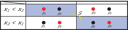
We will denote S⁡(y,p)≡SII,I​(y,p)S(y,p)\equiv S^{\mathrm{II,I}}(y,p). We must check whether this construction is well defined in the sense that it respects (45). How this works is schematically depicted in Figure 1.
Refer to caption
Figure 1: Example of the construction of the coefficients in the different sectors. The black dots correspond to the bosons of the vacuum, W1W_{1}, and the red dots correspond to the inserted fermions. The construction is well-defined if, by acting on the coefficient in the upper left quadrant by the S-matrix, one obtains the coefficient in the lower right quadrant.

By the factorization property of the S-matrix, it suffices to restrict to a two particle state and a two particle S-matrix. For this case (45) gives the following equations

ei​p12ei​p22​η⁡(p2)η⁡(p1)​x1+−x1−x1+−x2−​f​(y,p1)+ei​p12​x1−−x2−x1+−x2−​f​(y,p2)​S​(y,p1)\displaystyle\frac{e^{i\frac{p_{1}}{2}}}{e^{i\frac{p_{2}}{2}}}\frac{\eta(p_{2})}{\eta(p_{1})}\frac{x^{+}_{1}-x^{-}_{1}}{x^{+}_{1}-x^{-}_{2}}~f(y,p_{1})+e^{i\frac{p_{1}}{2}}\frac{x^{-}_{1}-x^{-}_{2}}{x^{+}_{1}-x^{-}_{2}}~f(y,p_{2})S(y,p_{1}) =\displaystyle= f⁡(y,p2)\displaystyle f(y,p_{2})
e−i​p22​x1+−x2+x1+−x2−​f​(y,p1)+η⁡(p1)η⁡(p2)​x2+−x2−x1+−x2−​f​(y,p2)​S​(y,p1)\displaystyle e^{-i\frac{p_{2}}{2}}\frac{x^{+}_{1}-x^{+}_{2}}{x^{+}_{1}-x^{-}_{2}}~f(y,p_{1})+\frac{\eta(p_{1})}{\eta(p_{2})}\frac{x^{+}_{2}-x^{-}_{2}}{x^{+}_{1}-x^{-}_{2}}~f(y,p_{2})S(y,p_{1}) =\displaystyle= f⁡(y,p1)​S​(y,p2).\displaystyle f(y,p_{1})S(y,p_{2}). (50)

These equations can be solved explicitly and the solution is given by:

f⁡(y,pk)\displaystyle f(y,p_{k}) =\displaystyle= η⁡(pk)​xk−xk+​yy−xk−​g​ℓk2\displaystyle\eta(p_{k})\sqrt{\frac{x^{-}_{k}}{x^{+}_{k}}}\frac{y}{y-x_{k}^{-}}\sqrt{\frac{g\ell_{k}}{2}}
S⁡(y,pk)\displaystyle S(y,p_{k}) =\displaystyle= xk−xk+​y−xk+y−xk−,\displaystyle\sqrt{\frac{x^{-}_{k}}{x^{+}_{k}}}\frac{y-x^{+}_{k}}{y-x_{k}^{-}}, (51)

where yy enters as a integration constant. With a modest amount of foresight, we choose the overall normalization of ff to be dependent on the bound state number ℓk\ell_{k}.

Actually this solution is the unique solution of (45) for one fermion in the vacuum up to overall normalization (and hence the only well-defined coefficient for this case). This can easily be seen from (50). The general wave function is of the form

|α⟩:=A1​Wα(1)​…​W1(K)+A2​W1(1)​Wα(2)​…​W1(K)+….\displaystyle|\alpha\rangle:=A_{1}W^{(1)}_{\alpha}\ldots W_{1}^{(K)}+A_{2}W^{(1)}_{1}W^{(2)}_{\alpha}\ldots W_{1}^{(K)}+\ldots. (52)

Since we are only interested in solving (44), the normalization of the state is irrelevant. Let us therefore pick a convenient normalization, A1≡f⁡(p1)A_{1}\equiv f(p_{1}), then by the first equation of (50) one finds A2A_{2} in terms of A1A_{1}. This indeed fixes A2A_{2} as f⁡(p2)​S​(p1)f(p_{2})S(p_{1}) and by induction the rest of the coefficients also follow. Finally, let us stress that by fixing the normalization, one automatically finds from the S-matrix that the other coefficients of the wave function are of a factorized form.

The problem becomes more involved upon inserting two excitations. In this case, it appears that the ansatz for the coefficient can be written as

|α​β⟩=|α​β⟩y1​y2+𝕊II​|α​β⟩y1​y2,\displaystyle|\alpha\beta\rangle=|\alpha\beta\rangle_{y_{1}y_{2}}+{\mathbb{S}}^{\mathrm{II}}|\alpha\beta\rangle_{y_{1}y_{2}}, (53)

where we introduce a new S-matrix 𝕊II{\mathbb{S}}^{\mathrm{II}}

𝕊II​|α​β⟩y1​y2\displaystyle{\mathbb{S}}^{\mathrm{II}}|\alpha\beta\rangle_{y_{1}y_{2}} =\displaystyle= M⁡(y1,y2)​|α​β⟩y2​y1+N⁡(y1,y2)​|β​α⟩y2​y1.\displaystyle M(y_{1},y_{2})|\alpha\beta\rangle_{y_{2}y_{1}}+N(y_{1},y_{2})|\beta\alpha\rangle_{y_{2}y_{1}}. (54)

Explicitly, it is given by

|α​β⟩\displaystyle|\alpha\beta\rangle =\displaystyle= ∑k<lΨk​(y1)​Ψl​(y2)​W1(1)​…​Wα(k)​…​Wβ(l)​…​W1(K)+\displaystyle\sum_{k<l}\Psi_{k}(y_{1})\Psi_{l}(y_{2})W^{(1)}_{1}\ldots W^{(k)}_{\alpha}\ldots W^{(l)}_{\beta}\ldots W_{1}^{(K)}+ (55)
+𝕊II∑k<lΨk(y1)Ψl(y2)W1(1)…Wα(k)…Wβ(l)…W1(K)+\displaystyle+{\mathbb{S}}^{\mathrm{II}}\sum_{k<l}\Psi_{k}(y_{1})\Psi_{l}(y_{2})W^{(1)}_{1}\ldots W^{(k)}_{\alpha}\ldots W^{(l)}_{\beta}\ldots W_{1}^{(K)}+
+ϵα​β∑kΨk(y1)Ψk(y2)h(y1,y2,pk)W1(1)…W2(k)…W1(K)\displaystyle+\epsilon^{\alpha\beta}\sum_{k}\Psi_{k}(y_{1})\Psi_{k}(y_{2})h(y_{1},y_{2},p_{k})W^{(1)}_{1}\ldots W^{(k)}_{2}\ldots W_{1}^{(K)}

When we restrict to just two sites, the wave function splits into the sum of a wave function with just one fermion. By construction, this piece is exactly as described above. The other piece contains two excitations and is given by

|α​β⟩\displaystyle|\alpha\beta\rangle =\displaystyle= {f⁡(y1,p1)​f​(y2,p2)​S​(y2,p1)+M​f​(y2,p1)​f​(y1,p2)​S​(y1,p1)}​Wα(1)​Wβ(2)\displaystyle\left\{f(y_{1},p_{1})f(y_{2},p_{2})S(y_{2},p_{1})+Mf(y_{2},p_{1})f(y_{1},p_{2})S(y_{1},p_{1})\right\}W^{(1)}_{\alpha}W^{(2)}_{\beta} (56)
+N​f​(y2,p1)​f​(y1,p2)​S​(y1,p1)​Wβ(1)​Wα(2)\displaystyle+Nf(y_{2},p_{1})f(y_{1},p_{2})S(y_{1},p_{1})W^{(1)}_{\beta}W^{(2)}_{\alpha}
+ϵα​β​h​(y1,y2,p1)​f​(y2,p1)​f​(y1,p1)​W2(1)​W1(2)\displaystyle+\epsilon^{\alpha\beta}h(y_{1},y_{2},p_{1})f(y_{2},p_{1})f(y_{1},p_{1})W^{(1)}_{2}W^{(2)}_{1}
+ϵα​β​h​(y1,y2,p2)​f​(y2,p2)​f​(y1,p2)​S​(y2,p1)​S​(y1,p1)​W1(1)​W2(2)\displaystyle+\epsilon^{\alpha\beta}h(y_{1},y_{2},p_{2})f(y_{2},p_{2})f(y_{1},p_{2})S(y_{2},p_{1})S(y_{1},p_{1})W^{(1)}_{1}W^{(2)}_{2}

Plugging this into (45) again allows one to find the explicit (unique) solutions of the unknown functions:

M⁡(y1,y2)\displaystyle M(y_{1},y_{2}) =\displaystyle= 2​i/gy1+1y1−y2−1y2−2​ig\displaystyle\frac{2i/g}{y_{1}+\frac{1}{y_{1}}-y_{2}-\frac{1}{y_{2}}-\frac{2i}{g}}
N⁡(y1,y2)\displaystyle N(y_{1},y_{2}) =\displaystyle= −y1+1y1−y2−1y2y1+1y1−y2−1y2−2​ig\displaystyle-\frac{y_{1}+\frac{1}{y_{1}}-y_{2}-\frac{1}{y_{2}}}{y_{1}+\frac{1}{y_{1}}-y_{2}-\frac{1}{y_{2}}-\frac{2i}{g}} (57)
h⁡(y1,y2,pk)\displaystyle h(y_{1},y_{2},p_{k}) =\displaystyle= iℓk​η​(pk)2​y1​y2−xk+​xk−y1​y2​xk+−xk−xk−​y1−y2y1+1y1−y2−1y2−2​ig\displaystyle\frac{i}{\ell_{k}\eta(p_{k})^{2}}~\frac{y_{1}y_{2}-x_{k}^{+}x_{k}^{-}}{y_{1}y_{2}}~\frac{x_{k}^{+}-x_{k}^{-}}{x^{-}_{k}}~\frac{y_{1}-y_{2}}{y_{1}+\frac{1}{y_{1}}-y_{2}-\frac{1}{y_{2}}-\frac{2i}{g}}

In this process, we introduced a new S-matrix and we also insist on naturalness of the wave function with respect to this S-matrix, 𝕊II{\mathbb{S}}^{\mathrm{II}}. One can repeat the above procedure to deal with this. For details we refer to [13, 8]. In this process we are again lead to introduce new functions SII,II,f(2),SIII,II,SIII,IIIS^{\mathrm{II,II}},f^{(2)},S^{\mathrm{III},\mathrm{II}},S^{\mathrm{III,III}}. The result of this consideration is

SII,II\displaystyle S^{\mathrm{II,II}} =\displaystyle= −M−N=1\displaystyle-M-N=1
f(2)​(w,yk)\displaystyle f^{(2)}(w,y_{k}) =\displaystyle= w−igw−vk−ig\displaystyle\frac{w-\frac{i}{g}}{w-v_{k}-\frac{i}{g}}
SIII,II​(w,yk)\displaystyle S^{\mathrm{III},\mathrm{II}}(w,y_{k}) =\displaystyle= w−vk+igw−vk−ig\displaystyle\frac{w-v_{k}+\frac{i}{g}}{w-v_{k}-\frac{i}{g}} (58)
SIII,III​(w1,w2)\displaystyle S^{\mathrm{III,III}}(w_{1},w_{2}) =\displaystyle= w1−w2−2​igw1−w2+2​ig,\displaystyle\frac{w_{1}-w_{2}-\frac{2i}{g}}{w_{1}-w_{2}+\frac{2i}{g}},

The Bethe equations (44) are formulated in terms of the factors used in the ansatz in the following way

ei​LA,k=∏B=IIII∏l=1KBSB​A​(xlB,xkA),(B,l)≠(A,k)\displaystyle e^{iL_{A,k}}={\prod_{B=\mathrm{I}}^{\mathrm{III}}\prod_{l=1}^{K^{B}}}S^{BA}(x^{B}_{l},x^{A}_{k}),\quad(B,l)\neq(A,k) (59)

where A,BA,B denote the different levels and SA​BS^{AB} can be seen as the S-matrix describing scattering at different levels. Moreover, ei​LI,k=e−i​L​pke^{iL_{\mathrm{I},k}}=e^{-iLp_{k}} and ei​LII,k=ei​LIII,k=1e^{iL_{\mathrm{II},k}}=e^{iL_{\mathrm{III},k}}=1 are phases.

By putting all of this together one obtains the well-known Bethe equations describing the asymptotic spectrum of the AdS5×S5{\rm AdS}_{5}\times{\rm S}^{5} superstring:

ei​pk​L\displaystyle e^{ip_{k}L} =\displaystyle= ∏l=1,l≠kKI[S0​(pk,pl)​xk+−xl−xk−−xl+​xl+​xk−xl−​xk+]2​∏α=12∏l=1K(α)IIxk−−yl(α)xk+−yl(α)​xk+xk−\displaystyle\prod_{l=1,l\neq k}^{K^{\mathrm{I}}}\left[S_{0}(p_{k},p_{l})\frac{x_{k}^{+}-x_{l}^{-}}{x_{k}^{-}-x_{l}^{+}}\sqrt{\frac{x_{l}^{+}x_{k}^{-}}{x_{l}^{-}x_{k}^{+}}}\right]^{2}\prod_{\alpha=1}^{2}\prod_{l=1}^{K_{(\alpha)}^{\mathrm{II}}}\frac{{x_{k}^{-}-y^{(\alpha)}_{l}}}{x_{k}^{+}-y^{(\alpha)}_{l}}\sqrt{\frac{x^{+}_{k}}{x^{-}_{k}}}
1\displaystyle 1 =\displaystyle= ∏l=1KIyk(α)−xl+yk(α)−xl−​xk−xk+​∏l=1K(α)IIIyk(α)+1yk(α)−wl(α)+igyk(α)+1yk(α)−wl(α)−ig\displaystyle\prod_{l=1}^{K^{\mathrm{I}}}\frac{y^{(\alpha)}_{k}-x^{+}_{l}}{y^{(\alpha)}_{k}-x^{-}_{l}}\sqrt{\frac{x^{-}_{k}}{x^{+}_{k}}}\prod_{l=1}^{K_{(\alpha)}^{\mathrm{III}}}\frac{y_{k}^{(\alpha)}+\frac{1}{y_{k}^{(\alpha)}}-w_{l}^{(\alpha)}+\frac{i}{g}}{y_{k}^{(\alpha)}+\frac{1}{y_{k}^{(\alpha)}}-w_{l}^{(\alpha)}-\frac{i}{g}} (60)
1\displaystyle 1 =\displaystyle= ∏l=1K(α)IIwk(α)−yk(α)−1yk(α)+igwk(α)−yk(α)−1yk(α)−ig​∏l≠kK(α)IIIwk(α)−wl(α)−2​igwk(α)−wlα+2​ig,\displaystyle\prod_{l=1}^{K_{(\alpha)}^{\mathrm{II}}}\frac{w_{k}^{(\alpha)}-y_{k}^{(\alpha)}-\frac{1}{y_{k}^{(\alpha)}}+\frac{i}{g}}{w_{k}^{(\alpha)}-y_{k}^{(\alpha)}-\frac{1}{y_{k}^{(\alpha)}}-\frac{i}{g}}\prod_{l\neq k}^{K_{(\alpha)}^{\mathrm{III}}}\frac{w_{k}^{(\alpha)}-w_{l}^{(\alpha)}-\frac{2i}{g}}{w_{k}^{(\alpha)}-w_{l}^{\alpha}+\frac{2i}{g}},

where α=1,2\alpha=1,2 reflect the two copies of 𝔰​𝔲​(2|2)\mathfrak{su}(2|2) and S0​(pk,pl)S_{0}(p_{k},p_{l}) is the overall phase of the S-matrix.

Notice that in this construction, the explicit form of the S-matrix is used. However, since not all bound state S-matrices are known, one must approach this problem in a different way if one wishes to find their Bethe equations.

4 Bethe Ansatz and Yangian Symmetry

In this section we will generalize the above construction to arbitrary bound states. We will do this by considering coproducts of (Yangian) symmetry generators. This formulation allows us to solve (45) without knowing the explicit form of the involved bound state S-matrix. This will lead to the Bethe equations for arbitrary configurations of bound states.

4.1 Single excitations

We will again start by considering a single excitation in the vacuum

|0⟩=W1ℓ1(1)​…​W1ℓK(K).\displaystyle|0\rangle=W^{(1)}_{1^{\ell_{1}}}\ldots W^{(K)}_{1^{\ell_{K}}}. (61)

As noted above, it suffices to restrict to two bound state representations. The natural generalization of a single excitation wave function is:

|α⟩:=∑iΨi​(y)​W1ℓ1(1)​…​W31​1ℓi−1(i)​…​W1ℓK(K),Ψk​(y)=f⁡(y,pk)​∏l<kSI,II​(y,pl),\displaystyle|\alpha\rangle:=\sum_{i}\Psi_{i}(y)W^{(1)}_{1^{\ell_{1}}}\ldots W^{(i)}_{3^{1}1^{\ell_{i}-1}}\ldots W^{(K)}_{1^{\ell_{K}}},\qquad\Psi_{k}(y)=f(y,p_{k})\prod_{l<k}S^{\mathrm{I,II}}(y,p_{l}), (62)

Restricted to two sites, the wave function is of the form

|α⟩=f⁡(p1)​Wα​1ℓ1−1(1)​W1ℓ2(2)+f⁡(p2)​S​(p1)​W1ℓ1(1)​Wα​1ℓ2−1(2),\displaystyle|\alpha\rangle=f(p_{1})W^{(1)}_{\alpha 1^{\ell_{1}-1}}W^{(2)}_{1^{\ell_{2}}}+f(p_{2})S(p_{1})W^{(1)}_{1^{\ell_{1}}}W^{(2)}_{\alpha 1^{\ell_{2}-1}}, (63)

where we again have chosen a particular normalization. The remarkable fact is that one can write this as:

Δ~​ℚα1​|0⟩:=(K0​(p1,p2)​Δ​ℚα1+K1​(p1,p2)​Δ​ℚ^α1)​|0⟩,\displaystyle\tilde{\Delta}\mathbb{Q}^{1}_{\alpha}|0\rangle:=\left(K_{0}(p_{1},p_{2})\Delta\mathbb{Q}^{1}_{\alpha}+K_{1}(p_{1},p_{2})\Delta\hat{\mathbb{Q}}^{1}_{\alpha}\right)|0\rangle, (64)

with

K0\displaystyle K_{0} =−2gx2−​{x1−​x2−​(x1+​x2+−1)−x1+​x2+​(1+x1−​[x1−+x1++x2+])}(x2−−x1+)​(2​x1+​x2+​x1−​x2−−x1−​x2−−x1+​x2+)×\displaystyle=-\sqrt{\frac{2}{g}}\frac{x_{2}^{-}\{x_{1}^{-}x_{2}^{-}(x_{1}^{+}x_{2}^{+}-1)-x_{1}^{+}x_{2}^{+}(1+x_{1}^{-}[x_{1}^{-}+x_{1}^{+}+x_{2}^{+}])\}}{(x_{2}^{-}-x_{1}^{+})(2x_{1}^{+}x_{2}^{+}x_{1}^{-}x_{2}^{-}-x_{1}^{-}x_{2}^{-}-x_{1}^{+}x_{2}^{+})}\times (65)
×[f⁡(p2)​S​(p1)ℓ2​η​(p2)−e−i​p22​f​(p1)ℓ1​η​(p1)]+e−i​p22​f​(p1)ℓ1​η​(p1)\displaystyle\times\left[\frac{f(p_{2})S(p_{1})}{\sqrt{\ell_{2}}\eta(p_{2})}-\frac{e^{-i\frac{p_{2}}{2}}f(p_{1})}{\sqrt{\ell_{1}}\eta(p_{1})}\right]+\frac{e^{-i\frac{p_{2}}{2}}f(p_{1})}{\sqrt{\ell_{1}}\eta(p_{1})}
K1\displaystyle K_{1} =4​i​2g3/2​x1−​x2−​x1+​x2+(x2−−x1+)​(2​x1+​x2+​x1−​x2−−x1−​x2−−x1+​x2+)​[f⁡(p2)​S​(p1)ℓ2​η​(p2)−e−i​p22​f​(p1)ℓ1​η​(p1)]\displaystyle=\frac{4i\sqrt{2}}{g^{3/2}}\frac{x_{1}^{-}x_{2}^{-}x_{1}^{+}x_{2}^{+}}{(x_{2}^{-}-x_{1}^{+})(2x_{1}^{+}x_{2}^{+}x_{1}^{-}x_{2}^{-}-x_{1}^{-}x_{2}^{-}-x_{1}^{+}x_{2}^{+})}\left[\frac{f(p_{2})S(p_{1})}{\sqrt{\ell_{2}}\eta(p_{2})}-\frac{e^{-i\frac{p_{2}}{2}}f(p_{1})}{\sqrt{\ell_{1}}\eta(p_{1})}\right]

For the moment let us keep f,Sf,S arbitrary. The invariance of the S-matrix under Yangian symmetry means that

𝕊​Δ​ℚα1=Δo​p​ℚα1​𝕊,𝕊​Δ​ℚ^α1=Δo​p​ℚ^α1​𝕊.\displaystyle{\mathbb{S}}\Delta\mathbb{Q}^{1}_{\alpha}=\Delta^{op}\mathbb{Q}^{1}_{\alpha}{\mathbb{S}},\qquad{\mathbb{S}}\Delta\hat{\mathbb{Q}}^{1}_{\alpha}=\Delta^{op}\hat{\mathbb{Q}}^{1}_{\alpha}{\mathbb{S}}. (66)

In other words, we find:

𝕊​|α⟩\displaystyle{\mathbb{S}}|\alpha\rangle =\displaystyle= 𝕊⁡(K0​(p1,p2)​Δ​ℚα1+K1​(p1,p2)​Δ​ℚ^α1)​|0⟩\displaystyle{\mathbb{S}}\left(K_{0}(p_{1},p_{2})\Delta\mathbb{Q}^{1}_{\alpha}+K_{1}(p_{1},p_{2})\Delta\hat{\mathbb{Q}}^{1}_{\alpha}\right)|0\rangle (67)
=\displaystyle= (K0​(p1,p2)​Δo​p​ℚα1+K1​(p1,p2)​Δo​p​ℚ^α1)​𝕊​|0⟩\displaystyle\left(K_{0}(p_{1},p_{2})\Delta^{op}\mathbb{Q}^{1}_{\alpha}+K_{1}(p_{1},p_{2})\Delta^{op}\hat{\mathbb{Q}}^{1}_{\alpha}\right){\mathbb{S}}|0\rangle
=\displaystyle= (K0​(p1,p2)​Δo​p​ℚα1+K1​(p1,p2)​Δo​p​ℚ^α1)​|0⟩,\displaystyle\left(K_{0}(p_{1},p_{2})\Delta^{op}\mathbb{Q}^{1}_{\alpha}+K_{1}(p_{1},p_{2})\Delta^{op}\hat{\mathbb{Q}}^{1}_{\alpha}\right)|0\rangle, (68)

since 𝕊​|0⟩=|0⟩{\mathbb{S}}|0\rangle=|0\rangle. However, we also have

|α⟩π\displaystyle|\alpha\rangle_{\pi} =\displaystyle= (K0​(p2,p1)​Δo​p​ℚα1+K1​(p2,p1)​Δo​p​ℚ^α1)​|0⟩.\displaystyle\left(K_{0}(p_{2},p_{1})\Delta^{op}\mathbb{Q}^{1}_{\alpha}+K_{1}(p_{2},p_{1})\Delta^{op}\hat{\mathbb{Q}}^{1}_{\alpha}\right)|0\rangle. (69)

This means that (45) corresponds to requiring that K0K_{0} and K1K_{1} are symmetric under interchanging p1↔p2p_{1}\leftrightarrow p_{2}. In other words, to find a well-defined coefficient, we have to solve

K0​(p1,p2)=K0​(p2,p1),K1​(p1,p2)=K1​(p2,p1),\displaystyle K_{0}(p_{1},p_{2})=K_{0}(p_{2},p_{1}),\qquad K_{1}(p_{1},p_{2})=K_{1}(p_{2},p_{1}), (70)

for the functions ff and SS.

It is straightforward to prove that (70) is equivalent to the equations:

K​f​(p1)+G​f​(p2)​S​(p1)\displaystyle Kf(p_{1})+Gf(p_{2})S(p_{1}) =\displaystyle= f⁡(p2)\displaystyle f(p_{2})
L​f​(p1)+H​f​(p2)​S​(p1)\displaystyle Lf(p_{1})+Hf(p_{2})S(p_{1}) =\displaystyle= f⁡(p1)​S​(p2),\displaystyle f(p_{1})S(p_{2}), (71)

with

K=ei​p12ei​p22​ℓ2​η​(p2)ℓ1​η​(p1)​x1+−x1−x1+−x2−G=ei​p12​x1−−x2−x1+−x2−L=e−i​p22​x1+−x2+x1+−x2−H=ℓ1​η​(p1)ℓ2​η​(p2)​x2+−x2−x1+−x2−.\displaystyle\begin{array}[]{lll}K=\frac{e^{i\frac{p_{1}}{2}}}{e^{i\frac{p_{2}}{2}}}\frac{\sqrt{\ell_{2}}\eta(p_{2})}{\sqrt{\ell_{1}}\eta(p_{1})}\frac{x^{+}_{1}-x^{-}_{1}}{x^{+}_{1}-x^{-}_{2}}&&G=e^{i\frac{p_{1}}{2}}\frac{x^{-}_{1}-x^{-}_{2}}{x^{+}_{1}-x^{-}_{2}}\\ L=e^{-i\frac{p_{2}}{2}}\frac{x^{+}_{1}-x^{+}_{2}}{x^{+}_{1}-x^{-}_{2}}&&H=\frac{\sqrt{\ell_{1}}\eta(p_{1})}{\sqrt{\ell_{2}}\eta(p_{2})}\frac{x^{+}_{2}-x^{-}_{2}}{x^{+}_{1}-x^{-}_{2}}\end{array}.

These equations are solved by the f,Sf,S found before, i.e. we again find (51) as unique solution. The discussion from the previous section holds also here. By fixing the normalization of the first term to be f⁡(p1)f(p_{1}), one finds that the second term is factorized and fixed.

Moreover, notice that from this construction we can read off elements of the S-matrix. Namely, the coefficients that deal with the scattering of Wα​aℓ1−1(1)​Waℓ2(2)W^{(1)}_{\alpha a^{\ell_{1}-1}}W^{(2)}_{a^{\ell_{2}}} and Waℓ1(1)​Wα​aℓ2−1(2)W^{(1)}_{a^{\ell_{1}}}W^{(2)}_{\alpha a^{\ell_{2}-1}}. We compared the found coefficients with the explicit known S-matrices and we indeed find perfect agreement. For example, for 𝕊B​B{\mathbb{S}}^{BB} they coincide with a9,a10,a31a_{9},a_{10},a_{31} and a32a_{32}, cf. [27].

In conclusion, symmetry of the coefficients uniquely fixes the form of our wave function. We can now write the wave function, restricted to two sites, completely in terms of coproducts and as a consequence (45) is automatically satisfied. Finally, the explicit expressions for K0,K1K_{0},K_{1} are

K0​(p1,p2,y)\displaystyle K_{0}(p_{1},p_{2},y) =\displaystyle= x1−x1+​x2−x2+​y(y−x1−)​(y−x2−)​[y−x1−​x2−​x1+​x2+​(x1−+x2−+x1++x2+)2​x1−​x2−​x1+​x2+−x1−​x2−−x1+​x2+]\displaystyle\sqrt{\frac{x_{1}^{-}}{x_{1}^{+}}}\sqrt{\frac{x_{2}^{-}}{x_{2}^{+}}}\frac{y}{(y-x_{1}^{-})(y-x_{2}^{-})}\left[y-\frac{x_{1}^{-}x_{2}^{-}x_{1}^{+}x_{2}^{+}(x_{1}^{-}+x_{2}^{-}+x_{1}^{+}+x_{2}^{+})}{2x_{1}^{-}x_{2}^{-}x_{1}^{+}x_{2}^{+}-x_{1}^{-}x_{2}^{-}-x_{1}^{+}x_{2}^{+}}\right]
K1​(p1,p2,y)\displaystyle K_{1}(p_{1},p_{2},y) =\displaystyle= 4​ig​x1−x1+​x2−x2+​y(y−x1−)​(y−x2−)​[x1−​x2−​x1+​x2+2​x1−​x2−​x1+​x2+−x1−​x2−−x1+​x2+].\displaystyle\frac{4i}{g}\sqrt{\frac{x_{1}^{-}}{x_{1}^{+}}}\sqrt{\frac{x_{2}^{-}}{x_{2}^{+}}}\frac{y}{(y-x_{1}^{-})(y-x_{2}^{-})}\left[\frac{x_{1}^{-}x_{2}^{-}x_{1}^{+}x_{2}^{+}}{2x_{1}^{-}x_{2}^{-}x_{1}^{+}x_{2}^{+}-x_{1}^{-}x_{2}^{-}-x_{1}^{+}x_{2}^{+}}\right]. (75)

This consideration is valid for any bound state numbers and hence wave function (62) is valid for any bound state representations. In particular, all bound state representations share the same SI,IIS^{\mathrm{I,II}}, and hence that part of the Bethe equations remains the same.

4.2 Multiple excitations

When dealing with two excitations, one needs to introduce a level II\mathrm{II} S-matrix that deals with interchanging y1y_{1} and y2y_{2}.

Fundamental representations

Let us first restrict to fundamental representations and reformulate this in terms of coproducts. The wave function was of the form

|α​β⟩=|α​β⟩y1​y2+𝕊II​|α​β⟩y1​y2,\displaystyle|\alpha\beta\rangle=|\alpha\beta\rangle_{y_{1}y_{2}}+{\mathbb{S}}^{\mathrm{II}}|\alpha\beta\rangle_{y_{1}y_{2}}, (76)

where

𝕊II​|α​β⟩y1​y2\displaystyle{\mathbb{S}}^{\mathrm{II}}|\alpha\beta\rangle_{y_{1}y_{2}} =\displaystyle= M⁡(y1,y2)​|α​β⟩y2​y1+N⁡(y1,y2)​|β​α⟩y2​y1.\displaystyle M(y_{1},y_{2})|\alpha\beta\rangle_{y_{2}y_{1}}+N(y_{1},y_{2})|\beta\alpha\rangle_{y_{2}y_{1}}. (77)

The natural way to write this would be:

|α​β⟩y1​y2\displaystyle|\alpha\beta\rangle_{y_{1}y_{2}} =\displaystyle= {(Δ~y1​ℚα1)​(Δ~y2​ℚβ1)+ϵα​β​Δy1,y2′​𝕃21}​|0⟩,\displaystyle\left\{(\tilde{\Delta}_{y_{1}}\mathbb{Q}^{1}_{\alpha})(\tilde{\Delta}_{y_{2}}\mathbb{Q}^{1}_{\beta})+\epsilon_{\alpha\beta}\Delta^{\prime}_{y_{1},y_{2}}\mathbb{L}^{1}_{2}\right\}|0\rangle, (78)

with

Δy1,y2′​𝕃21\displaystyle\Delta^{\prime}_{y_{1},y_{2}}\mathbb{L}^{1}_{2} :⁣=\displaystyle:= L0​(y1,y2,p1,p2)​Δ​𝕃21+L1​(y1,y2,p1,p2)​Δ​𝕃^21\displaystyle L_{0}(y_{1},y_{2},p_{1},p_{2})\Delta\mathbb{L}^{1}_{2}+L_{1}(y_{1},y_{2},p_{1},p_{2})\Delta\hat{\mathbb{L}}^{1}_{2} (79)

By taking α=β\alpha=\beta, one easily checks that the first part is indeed of the form (Δ~y1​ℚα1)​(Δ~y2​ℚβ1)(\tilde{\Delta}_{y_{1}}\mathbb{Q}^{1}_{\alpha})(\tilde{\Delta}_{y_{2}}\mathbb{Q}^{1}_{\beta}). Hence, we have to solve L0,L1L_{0},L_{1} such that our ansatz gives

{f⁡(y1,p1)​f​(y2,p2)​S​(y2,p1)+M​f​(y2,p1)​f​(y1,p2)​S​(y1,p1)}​Wα(1)​Wβ(2)\displaystyle\left\{f(y_{1},p_{1})f(y_{2},p_{2})S(y_{2},p_{1})+Mf(y_{2},p_{1})f(y_{1},p_{2})S(y_{1},p_{1})\right\}W^{(1)}_{\alpha}W^{(2)}_{\beta}
+N​f​(y2,p1)​f​(y1,p2)​S​(y1,p1)​Wβ(1)​Wα(2)\displaystyle+Nf(y_{2},p_{1})f(y_{1},p_{2})S(y_{1},p_{1})W^{(1)}_{\beta}W^{(2)}_{\alpha}
+ϵα​β​h​(y1,y2,p1)​f​(y2,p1)​f​(y1,p1)​W2(1)​W1(2)\displaystyle+\epsilon^{\alpha\beta}h(y_{1},y_{2},p_{1})f(y_{2},p_{1})f(y_{1},p_{1})W^{(1)}_{2}W^{(2)}_{1} (80)
+ϵα​β​h​(y1,y2,p2)​f​(y2,p2)​f​(y1,p2)​S​(y2,p1)​S​(y1,p1)​W1(1)​W2(2),\displaystyle+\epsilon^{\alpha\beta}h(y_{1},y_{2},p_{2})f(y_{2},p_{2})f(y_{1},p_{2})S(y_{2},p_{1})S(y_{1},p_{1})W^{(1)}_{1}W^{(2)}_{2},

where we keep the functions M,N,hM,N,h arbitrary. This gives two equations for L0L_{0} and two equations for L1L_{1}. Hence, requiring symmetry under p1↔p2p_{1}\leftrightarrow p_{2} will give us four equations which can be shown to be equivalent to the following set of equations:

{f12​f21​S22+M​f22​f11​S12}\displaystyle\{f_{12}f_{21}S_{22}+Mf_{22}f_{11}S_{12}\} =\displaystyle= {f11​f22​S21+M​f21​f12​S11}​D+E2+N​f21​f12​S11​D−E2\displaystyle\{f_{11}f_{22}S_{21}+Mf_{21}f_{12}S_{11}\}\frac{D+E}{2}+Nf_{21}f_{12}S_{11}\frac{D-E}{2}
+(−f11​f21​h121+f12​f22​S11​S21​h122)​C2\displaystyle+\left(-f_{11}f_{21}h_{121}+f_{12}f_{22}S_{11}S_{21}h_{122}\right)\frac{C}{2}
N​f22​f11​S12\displaystyle Nf_{22}f_{11}S_{12} =\displaystyle= {f11​f22​S21+M​f21​f12​S11}​D−E2+N​f21​f12​S11​D+E2\displaystyle\{f_{11}f_{22}S_{21}+Mf_{21}f_{12}S_{11}\}\frac{D-E}{2}+Nf_{21}f_{12}S_{11}\frac{D+E}{2}
−(−f11​f21​h121+f12​f22​S11​S21​h122)​C2.\displaystyle-\left(-f_{11}f_{21}h_{121}+f_{12}f_{22}S_{11}S_{21}h_{122}\right)\frac{C}{2}.
f11​f21​S12​S22​h121\displaystyle f_{11}f_{21}S_{12}S_{22}h_{121} =\displaystyle= {f11​f22​S21+(M−N)​f21​f12​S11}​F2\displaystyle\{f_{11}f_{22}S_{21}+(M-N)f_{21}f_{12}S_{11}\}\frac{F}{2} (81)
+f11​f21​h121​1−B2+f12​f22​S11​S21​h122​1+B2\displaystyle+f_{11}f_{21}h_{121}\frac{1-B}{2}+f_{12}f_{22}S_{11}S_{21}h_{122}\frac{1+B}{2}
f12​f22​h122\displaystyle f_{12}f_{22}h_{122} =\displaystyle= −{f11​f22​S21+(M−N)​f21​f12​S11}​F2\displaystyle-\{f_{11}f_{22}S_{21}+(M-N)f_{21}f_{12}S_{11}\}\frac{F}{2} (82)
+f11​f21​h121​1+B2+f12​f22​S11​S21​h122​1−B2,\displaystyle+f_{11}f_{21}h_{121}\frac{1+B}{2}+f_{12}f_{22}S_{11}S_{21}h_{122}\frac{1-B}{2},

where, for convenience, we introduced the short-hand notation fk​l:=f⁡(yk,pl),Sk​l:=SII,I​(yk,pl),M:=M⁡(y1,y2),N:=N⁡(y1,y2)f_{kl}:=f(y_{k},p_{l}),S_{kl}:=S^{\mathrm{II,I}}(y_{k},p_{l}),M:=M(y_{1},y_{2}),N:=N(y_{1},y_{2}) and hi​j​k:=h⁡(yi,yj,pk)h_{ijk}:=h(y_{i},y_{j},p_{k}). The coefficients B,C,D,E,FB,C,D,E,F are given by

B\displaystyle B =\displaystyle= 2​x1−​x2−​(x2+)2−(x1−​x2−+1)​(x2−+x1+)​x2++2​x2−​x1+(1−x1−​x2−)​(x1+−x2−)​x2+\displaystyle\frac{2x_{1}^{-}x_{2}^{-}(x_{2}^{+})^{2}-(x_{1}^{-}x_{2}^{-}+1)(x_{2}^{-}+x_{1}^{+})x_{2}^{+}+2x_{2}^{-}x_{1}^{+}}{(1-x_{1}^{-}x_{2}^{-})(x_{1}^{+}-x_{2}^{-})x_{2}^{+}}
C\displaystyle C =\displaystyle= 2​i​η​(p1)​η​(p2)​x2−x2+​e−i​p12​(x2+−x1+)(1−x1−​x2−)​(x1+−x2−)\displaystyle 2i\eta(p_{1})\eta(p_{2})\frac{x_{2}^{-}}{x_{2}^{+}}\frac{e^{-\frac{ip_{1}}{2}}(x_{2}^{+}-x_{1}^{+})}{(1-x_{1}^{-}x_{2}^{-})(x_{1}^{+}-x_{2}^{-})}
D\displaystyle D =\displaystyle= x1−−x2+x2−−x1+​ei​p12ei​p22\displaystyle\frac{x_{1}^{-}-x_{2}^{+}}{x_{2}^{-}-x_{1}^{+}}\frac{e^{\frac{ip_{1}}{2}}}{e^{\frac{ip_{2}}{2}}} (83)
E\displaystyle E =\displaystyle= ei​p12ei​p22​(x1−​(x2−​(x1−−2​x1+)+1)​x1++(x1++x1−​(x2−​x1+−2))​x2+)(1−x1−​x2−)​(x1+−x2−)​x1+\displaystyle\frac{e^{\frac{ip_{1}}{2}}}{e^{\frac{ip_{2}}{2}}}\frac{(x_{1}^{-}(x_{2}^{-}(x_{1}^{-}-2x_{1}^{+})+1)x_{1}^{+}+(x_{1}^{+}+x_{1}^{-}(x_{2}^{-}x_{1}^{+}-2))x_{2}^{+})}{(1-x_{1}^{-}x_{2}^{-})(x_{1}^{+}-x_{2}^{-})x_{1}^{+}}
F\displaystyle F =\displaystyle= 2​i​e−i​p12η⁡(p1)​η​(p2)​(x1+−x1−)​(x2+−x2−)​(x2+−x1+)(1−x1−​x2−)​(x1+−x2−).\displaystyle 2i\frac{e^{-\frac{ip_{1}}{2}}}{\eta(p_{1})\eta(p_{2})}\frac{(x_{1}^{+}-x_{1}^{-})(x_{2}^{+}-x_{2}^{-})(x_{2}^{+}-x_{1}^{+})}{(1-x_{1}^{-}x_{2}^{-})(x_{1}^{+}-x_{2}^{-})}.

It is readily seen that these expressions coincide with elements from the fundamental S-matrix. Remarkably, these are exactly the same equations that arose in the nested Bethe Ansatz. In other words, the coefficients B,C,D,E,FB,C,D,E,F correspond to elements from the fundamental S-matrix and we again find (57) as the unique solution for M,N,hM,N,h.

It is worthwhile to note that in this way, we have derived the complete fundamental S-matrix. This derivation differs fundamentally from the standard derivations [11, 8] since it depends crucially on the full Yangian symmetry. There might be a relation with [44] where the fundamental quantum S-matrix was also derived from Yangian symmetry.

To conclude, let us give the explicit solutions for L0,L1L_{0},L_{1},

L0\displaystyle L_{0} =g⁡(y1−y2)​x1−​x2−2​i​(y1−x1−)​(y2−x1−)​(y1−x2−)​(y2−x2−)×\displaystyle=\frac{g(y_{1}-y_{2})x^{-}_{1}x^{-}_{2}}{2i(y_{1}-x^{-}_{1})(y_{2}-x^{-}_{1})(y_{1}-x^{-}_{2})(y_{2}-x^{-}_{2})}\times (84)
×[(y1+y2)−x1−​x2−​x1+​x2+​(x1−+x2−+x1++x2+)2​x1+​x2+​x1−​x2−−x1−​x2−−x1+​x2+−y1​y2​x1+​x2+2​x1+​x2+​x1−​x2−−x1−​x2−−x1+​x2+{\displaystyle\times\left[(y_{1}+y_{2})-\frac{x^{-}_{1}x^{-}_{2}x^{+}_{1}x^{+}_{2}(x^{-}_{1}+x^{-}_{2}+x^{+}_{1}+x^{+}_{2})}{2x_{1}^{+}x_{2}^{+}x_{1}^{-}x_{2}^{-}-x_{1}^{-}x_{2}^{-}-x_{1}^{+}x_{2}^{+}}-\frac{y_{1}y_{2}x^{+}_{1}x^{+}_{2}}{2x_{1}^{+}x_{2}^{+}x_{1}^{-}x_{2}^{-}-x_{1}^{-}x_{2}^{-}-x_{1}^{+}x_{2}^{+}}\right\{
(x1++x2+−x1−−x2−)(x1−x2−−x1+x2+)−(1x2−+1x1++1x2++1x1−)(x1−x2−+x1+x2+)}]\displaystyle(x^{+}_{1}+x^{+}_{2}-x^{-}_{1}-x^{-}_{2})(x^{-}_{1}x^{-}_{2}-x^{+}_{1}x^{+}_{2})\left.\left.-\left(\frac{1}{x^{-}_{2}}+\frac{1}{x^{+}_{1}}+\frac{1}{x^{+}_{2}}+\frac{1}{x^{-}_{1}}\right)(x^{-}_{1}x^{-}_{2}+x^{+}_{1}x^{+}_{2})\right\}\right]
L1\displaystyle L_{1} =y1​y2​x1−​x2−(y1−x1−)​(y2−x1−)​(y1−x2−)​(y2−x2−)​[(y1−y2)+4​i​g−1​x1−​x2−​x1+​x2+2​x1+​x2+​x1−​x2−−x1−​x2−−x1+​x2+]\displaystyle=\frac{y_{1}y_{2}x^{-}_{1}x^{-}_{2}}{(y_{1}-x^{-}_{1})(y_{2}-x^{-}_{1})(y_{1}-x^{-}_{2})(y_{2}-x^{-}_{2})}\left[(y_{1}-y_{2})+\frac{4ig^{-1}x^{-}_{1}x^{-}_{2}x^{+}_{1}x^{+}_{2}}{2x_{1}^{+}x_{2}^{+}x_{1}^{-}x_{2}^{-}-x_{1}^{-}x_{2}^{-}-x_{1}^{+}x_{2}^{+}}\right]

Note that they are indeed manifestly symmetric under p1↔p2p_{1}\leftrightarrow p_{2}.

Bound states

One might hope that it is possible to repeat the construction of previous section and find explicit elements of the bound state S-matrices again. However, when considering bound states, one encounters a difficulty. There is a new term, which is of the form Wα​β​1ℓ1−2(i)W^{(i)}_{\alpha\beta 1^{\ell_{1}-2}}. This term behaves exactly like W21ℓ1−1(i)W^{(i)}_{21^{\ell_{1}-1}} and therefore it is hard to rewrite rewrite everything as in (81) in a unique way and read of S-matrix elements.

Nevertheless, we redo the procedure and try to match (78) to the obvious generalization of the two excitation ansatz

|α​β⟩\displaystyle|\alpha\beta\rangle =\displaystyle= ∑k<lΨk​(y1)​Ψl​(y2)​W1ℓ1(1)​…​Wα​1ℓk−1(k)​…​Wβ​1ℓl−1(l)​…​W1ℓK(K)+\displaystyle\sum_{k<l}\Psi_{k}(y_{1})\Psi_{l}(y_{2})W^{(1)}_{1^{\ell_{1}}}\ldots W^{(k)}_{\alpha 1^{\ell_{k}-1}}\ldots W^{(l)}_{\beta 1^{\ell_{l}-1}}\ldots W_{1^{\ell_{K}}}^{(K)}+ (86)
+𝕊II∑k<lΨk(y1)Ψl(y2)W1ℓ1(1)…Wα​1ℓk−1(k)…Wβ​1ℓl−1(l)…W1ℓK(K)+\displaystyle+{\mathbb{S}}^{\mathrm{II}}\sum_{k<l}\Psi_{k}(y_{1})\Psi_{l}(y_{2})W^{(1)}_{1^{\ell_{1}}}\ldots W^{(k)}_{\alpha 1^{\ell_{k}-1}}\ldots W^{(l)}_{\beta 1^{\ell_{l}-1}}\ldots W_{1^{\ell_{K}}}^{(K)}+
+ϵα​β∑kΨk(y1)Ψk(y2)h(y1,y2,pk)W1ℓ1(1)…W21ℓk−1(k)…W1ℓK(K)+\displaystyle+\epsilon^{\alpha\beta}\sum_{k}\Psi_{k}(y_{1})\Psi_{k}(y_{2})h(y_{1},y_{2},p_{k})W^{(1)}_{1^{\ell_{1}}}\ldots W^{(k)}_{21^{\ell_{k}-1}}\ldots W_{1^{\ell_{K}}}^{(K)}+
+∑kΨk(y1)Ψk(y2)g(y1,y2,pk)W1ℓ1(1)…Wα​β​1ℓk−2(k)…W1ℓK(K).\displaystyle+\sum_{k}\Psi_{k}(y_{1})\Psi_{k}(y_{2})g(y_{1},y_{2},p_{k})W^{(1)}_{1^{\ell_{1}}}\ldots W^{(k)}_{\alpha\beta 1^{\ell_{k}-2}}\ldots W_{1^{\ell_{K}}}^{(K)}.

Or, restricted to two sites

|α​β⟩\displaystyle|\alpha\beta\rangle =\displaystyle= {f⁡(y1,p1)​f​(y2,p2)​S​(y2,p1)+M​f​(y2,p1)​f​(y1,p2)​S​(y1,p1)}​Wα​1ℓ1−1(1)​Wβ​1ℓ2−1(2)\displaystyle\left\{f(y_{1},p_{1})f(y_{2},p_{2})S(y_{2},p_{1})+Mf(y_{2},p_{1})f(y_{1},p_{2})S(y_{1},p_{1})\right\}W^{(1)}_{\alpha 1^{\ell_{1}-1}}W^{(2)}_{\beta 1^{\ell_{2}-1}} (87)
+N​f​(y2,p1)​f​(y1,p2)​S​(y1,p1)​Wβ​1ℓ1−1(1)​Wα​1ℓ2−1(2)\displaystyle+Nf(y_{2},p_{1})f(y_{1},p_{2})S(y_{1},p_{1})W^{(1)}_{\beta 1^{\ell_{1}-1}}W^{(2)}_{\alpha 1^{\ell_{2}-1}}
+g⁡(y1,y2,p1)​f​(y1,p1)​f​(y2,p1)​Wα​βℓ1−2(1)​W1ℓ2(2)\displaystyle+g(y_{1},y_{2},p_{1})f(y_{1},p_{1})f(y_{2},p_{1})W^{(1)}_{\alpha\beta^{\ell_{1}-2}}W^{(2)}_{1^{\ell_{2}}}
+g⁡(y1,y2,p2)​f​(y2,p2)​f​(y1,p2)​S​(y1,p1)​S​(y2,p1)​W1ℓ1(1)​Wα​βℓ2−2(2)\displaystyle+g(y_{1},y_{2},p_{2})f(y_{2},p_{2})f(y_{1},p_{2})S(y_{1},p_{1})S(y_{2},p_{1})W^{(1)}_{1^{\ell_{1}}}W^{(2)}_{\alpha\beta^{\ell_{2}-2}}
+ϵα​β​h​(y1,y2,p1)​f​(y2,p1)​f​(y1,p1)​W21ℓ1−1(1)​W1ℓ2(2)\displaystyle+\epsilon^{\alpha\beta}h(y_{1},y_{2},p_{1})f(y_{2},p_{1})f(y_{1},p_{1})W^{(1)}_{21^{\ell_{1}-1}}W^{(2)}_{1^{\ell_{2}}}
+ϵα​β​h​(y1,y2,p2)​f​(y2,p2)​f​(y1,p2)​S​(y2,p1)​S​(y1,p1)​W1ℓ1(1)​W21ℓ2−1(2),\displaystyle+\epsilon^{\alpha\beta}h(y_{1},y_{2},p_{2})f(y_{2},p_{2})f(y_{1},p_{2})S(y_{2},p_{1})S(y_{1},p_{1})W^{(1)}_{1^{\ell_{1}}}W^{(2)}_{21^{\ell_{2}-1}},

This is indeed possible and imposing symmetry of L0,L1L_{0},L_{1} as before provides equations that are uniquely solved by g⁡(y1,y2,pk)=ℓk−12​ℓk​(1+M−N)g(y_{1},y_{2},p_{k})=\frac{\ell_{k}-1}{2\ell_{k}}(1+M-N) and (57). These factor are, more or less, expected from fusion. Plugging these solutions back in L0,L1L_{0},L_{1}, we find the same functions L0,L1L_{0},L_{1} as in (84) but one has to bear in mind that now x±x^{\pm} parameterize bound state solutions.

For completeness, we give the explicit two particle wave function (restricted to two sites) :

|α​β⟩\displaystyle|\alpha\beta\rangle =\displaystyle= {f⁡(y1,p1)​f​(y2,p2)​S​(y2,p1)+M​f​(y2,p1)​f​(y1,p2)​S​(y1,p1)}​Wα​1ℓ1−1(1)​Wβ​1ℓ2−1(2)\displaystyle\left\{f(y_{1},p_{1})f(y_{2},p_{2})S(y_{2},p_{1})+Mf(y_{2},p_{1})f(y_{1},p_{2})S(y_{1},p_{1})\right\}W^{(1)}_{\alpha 1^{\ell_{1}-1}}W^{(2)}_{\beta 1^{\ell_{2}-1}} (88)
+N​f​(y2,p1)​f​(y1,p2)​S​(y1,p1)​Wβ​1ℓ1−1(1)​Wα​1ℓ2−1(2)\displaystyle+Nf(y_{2},p_{1})f(y_{1},p_{2})S(y_{1},p_{1})W^{(1)}_{\beta 1^{\ell_{1}-1}}W^{(2)}_{\alpha 1^{\ell_{2}-1}}
+ℓ1−12​ℓ1​(1+M−N)​f​(y1,p1)​f​(y2,p1)​Wα​βℓ1−2(1)​W1ℓ2(2)\displaystyle+\frac{\ell_{1}-1}{2\ell_{1}}(1+M-N)f(y_{1},p_{1})f(y_{2},p_{1})W^{(1)}_{\alpha\beta^{\ell_{1}-2}}W^{(2)}_{1^{\ell_{2}}}
+ℓ2−12​ℓ2​(1+M−N)​f​(y1,p2)​f​(y2,p2)​S​(y1,p1)​S​(y2,p1)​W1ℓ1(1)​Wα​βℓ2−2(2)\displaystyle+\frac{\ell_{2}-1}{2\ell_{2}}(1+M-N)f(y_{1},p_{2})f(y_{2},p_{2})S(y_{1},p_{1})S(y_{2},p_{1})W^{(1)}_{1^{\ell_{1}}}W^{(2)}_{\alpha\beta^{\ell_{2}-2}}
+ϵα​β​h​(y1,y2,p1)​f​(y2,p1)​f​(y1,p1)​W21ℓ1−1(1)​W1ℓ2(2)\displaystyle+\epsilon^{\alpha\beta}h(y_{1},y_{2},p_{1})f(y_{2},p_{1})f(y_{1},p_{1})W^{(1)}_{21^{\ell_{1}-1}}W^{(2)}_{1^{\ell_{2}}}
+ϵα​β​h​(y1,y2,p2)​f​(y2,p2)​f​(y1,p2)​S​(y2,p1)​S​(y1,p1)​W1ℓ1(1)​W21ℓ2−1(2),\displaystyle+\epsilon^{\alpha\beta}h(y_{1},y_{2},p_{2})f(y_{2},p_{2})f(y_{1},p_{2})S(y_{2},p_{1})S(y_{1},p_{1})W^{(1)}_{1^{\ell_{1}}}W^{(2)}_{21^{\ell_{2}-1}},

with f,S,h,M,Nf,S,h,M,N as in (51,57). By construction, this wave function satisfies (45) for any bound state S-matrix. Hence this solves our two excitation case. In particular one finds that also the level II S-matrix, 𝕊II{\mathbb{S}}^{\mathrm{II}} is unchanged for bound states.

4.3 Bethe equations

By making use of coproducts and Yangian symmetry, we have found a way, independent of the explicit form of the S-matrix, to write down Bethe wave functions. This allowed us to find SII,IS^{\mathrm{II,I}} and we found that the level two S-matrix, 𝕊II{\mathbb{S}}^{\mathrm{II}} remains unchanged. Hence all the higher level factors also remain unchanged. In other words, this yields that the Bethe equations for any combination of bound states are given by:

ei​pk​L\displaystyle e^{ip_{k}L} =\displaystyle= ∏l=1,l≠kKI[S0​(pk,pl)​xk+−xl−xk−−xl+​xl+​xk−xl−​xk+]2​∏α=12∏l=1K(α)IIxk−−yl(α)xk+−yl(α)​xk+xk−\displaystyle\prod_{l=1,l\neq k}^{K^{\mathrm{I}}}\left[S_{0}(p_{k},p_{l})\frac{x_{k}^{+}-x_{l}^{-}}{x_{k}^{-}-x_{l}^{+}}\sqrt{\frac{x_{l}^{+}x_{k}^{-}}{x_{l}^{-}x_{k}^{+}}}\right]^{2}\prod_{\alpha=1}^{2}\prod_{l=1}^{K_{(\alpha)}^{\mathrm{II}}}\frac{{x_{k}^{-}-y^{(\alpha)}_{l}}}{x_{k}^{+}-y^{(\alpha)}_{l}}\sqrt{\frac{x^{+}_{k}}{x^{-}_{k}}}
1\displaystyle 1 =\displaystyle= ∏l=1KIyk(α)−xl+yk(α)−xl−​xk−xk+​∏l=1K(α)IIIyk(α)+1yk(α)−wl(α)+igyk(α)+1yk(α)−wl(α)−ig\displaystyle\prod_{l=1}^{K^{\mathrm{I}}}\frac{y^{(\alpha)}_{k}-x^{+}_{l}}{y^{(\alpha)}_{k}-x^{-}_{l}}\sqrt{\frac{x^{-}_{k}}{x^{+}_{k}}}\prod_{l=1}^{K_{(\alpha)}^{\mathrm{III}}}\frac{y_{k}^{(\alpha)}+\frac{1}{y_{k}^{(\alpha)}}-w_{l}^{(\alpha)}+\frac{i}{g}}{y_{k}^{(\alpha)}+\frac{1}{y_{k}^{(\alpha)}}-w_{l}^{(\alpha)}-\frac{i}{g}} (89)
1\displaystyle 1 =\displaystyle= ∏l=1K(α)IIwk(α)−yk(α)−1yk(α)+igwk(α)−yk(α)−1yk(α)−ig​∏l≠kK(α)IIIwk(α)−wl(α)−2​igwk(α)−wlα+2​ig,\displaystyle\prod_{l=1}^{K_{(\alpha)}^{\mathrm{II}}}\frac{w_{k}^{(\alpha)}-y_{k}^{(\alpha)}-\frac{1}{y_{k}^{(\alpha)}}+\frac{i}{g}}{w_{k}^{(\alpha)}-y_{k}^{(\alpha)}-\frac{1}{y_{k}^{(\alpha)}}-\frac{i}{g}}\prod_{l\neq k}^{K_{(\alpha)}^{\mathrm{III}}}\frac{w_{k}^{(\alpha)}-w_{l}^{(\alpha)}-\frac{2i}{g}}{w_{k}^{(\alpha)}-w_{l}^{\alpha}+\frac{2i}{g}},

with

xk++1xk+−xk−−1xk−=2​i​ℓkg,xk+xk−=ei​pk.\displaystyle x_{k}^{+}+\frac{1}{x_{k}^{+}}-x_{k}^{-}-\frac{1}{x_{k}^{-}}=\frac{2i\ell_{k}}{g},\qquad\frac{x_{k}^{+}}{x_{k}^{-}}=e^{ip_{k}}. (90)

However, note that apart from the parameters x±x^{\pm}, the phase factor S0​(pk,pl)S_{0}(p_{k},p_{l}) also implicitly depends on the considered bound states via [27]:

S0​(p1,p2)\displaystyle S_{0}(p_{1},p_{2}) =\displaystyle= (x1−x1+)ℓ22(x2+x2−)ℓ12σ(x1,x2)×\displaystyle\left(\frac{x_{1}^{-}}{x_{1}^{+}}\right)^{\frac{\ell_{2}}{2}}\left(\frac{x_{2}^{+}}{x_{2}^{-}}\right)^{\frac{\ell_{1}}{2}}\sigma(x_{1},x_{2})\times (91)
×G⁡(ℓ2−ℓ1)​G​(ℓ2+ℓ1)​∏l=1ℓ1−1G⁡(ℓ2−ℓ1+2​l).\displaystyle\times\sqrt{G(\ell_{2}-\ell_{1})G(\ell_{2}+\ell_{1})}\prod_{l=1}^{\ell_{1}-1}G(\ell_{2}-\ell_{1}+2l).

The derived Bethe equations coincide with the equations one expects from a fusion procedure. This justifies a fusion procedure at the level of the Bethe ansatz equations.

Finally, we will present the Bethe equations in the mirror theory since they will have applications there for the TBA program. In the mirror theory the parameters a,b,c,da,b,c,d describing the symmetry algebra have the same dependence on x±x^{\pm} as in the original theory. However x±x^{\pm} are now dependent on the mirror momentum

xi±​(p~)=ℓi2​g​(−1+4​g2ℓi2+p~2∓1)​(−p~ℓi−i).\displaystyle x_{i}^{\pm}(\tilde{p})=\frac{\ell_{i}}{2g}\left(-\sqrt{1+\frac{4g^{2}}{\ell_{i}^{2}+\tilde{p}^{2}}}\mp 1\right)\left(-\frac{\tilde{p}}{\ell_{i}}-i\right). (92)

To analyze bound states in the mirror theory it is more convenient to pick up a vacuum build up out of fermions (𝔰​𝔩​(2)\mathfrak{sl}(2) sector). The derivation can be repeated for this case and the Bethe equations are given by [23]

ei​p~k​L\displaystyle e^{i\tilde{p}_{k}L} =\displaystyle= ∏l=1,l≠kKIS0​(p~k,p~l)2​∏α=12∏l=1K(α)IIxk+−yl(α)xk−−yl(α)​xk−xk+\displaystyle\prod_{l=1,l\neq k}^{K^{\mathrm{I}}}S_{0}(\tilde{p}_{k},\tilde{p}_{l})^{2}\prod_{\alpha=1}^{2}\prod_{l=1}^{K_{(\alpha)}^{\mathrm{II}}}\frac{{x_{k}^{+}-y^{(\alpha)}_{l}}}{x_{k}^{-}-y^{(\alpha)}_{l}}\sqrt{\frac{x^{-}_{k}}{x^{+}_{k}}}
−1\displaystyle-1 =\displaystyle= ∏l=1KIyk(α)−xl+yk(α)−xl−​xk−xk+​∏l=1K(α)IIIyk(α)+1yk(α)−wl(α)+igyk(α)+1yk(α)−wl(α)−ig\displaystyle\prod_{l=1}^{K^{\mathrm{I}}}\frac{y^{(\alpha)}_{k}-x^{+}_{l}}{y^{(\alpha)}_{k}-x^{-}_{l}}\sqrt{\frac{x^{-}_{k}}{x^{+}_{k}}}\prod_{l=1}^{K_{(\alpha)}^{\mathrm{III}}}\frac{y_{k}^{(\alpha)}+\frac{1}{y_{k}^{(\alpha)}}-w_{l}^{(\alpha)}+\frac{i}{g}}{y_{k}^{(\alpha)}+\frac{1}{y_{k}^{(\alpha)}}-w_{l}^{(\alpha)}-\frac{i}{g}} (93)
1\displaystyle 1 =\displaystyle= ∏l=1K(α)IIwk(α)−yk(α)−1yk(α)+igwk(α)−yk(α)−1yk(α)−ig​∏l≠kK(α)IIIwk(α)−wl(α)−2​igwk(α)−wlα+2​ig,\displaystyle\prod_{l=1}^{K_{(\alpha)}^{\mathrm{II}}}\frac{w_{k}^{(\alpha)}-y_{k}^{(\alpha)}-\frac{1}{y_{k}^{(\alpha)}}+\frac{i}{g}}{w_{k}^{(\alpha)}-y_{k}^{(\alpha)}-\frac{1}{y_{k}^{(\alpha)}}-\frac{i}{g}}\prod_{l\neq k}^{K_{(\alpha)}^{\mathrm{III}}}\frac{w_{k}^{(\alpha)}-w_{l}^{(\alpha)}-\frac{2i}{g}}{w_{k}^{(\alpha)}-w_{l}^{\alpha}+\frac{2i}{g}},

where p~\tilde{p} is the mirror momentum and x±x^{\pm} are now given by (92). The −1-1 on the left hand side is due to anti-periodic boundary conditions for the fermions [23]. For a detailed account of the mirror theory and its analytic properties we refer to [23].

Acknowledgements

I am indebted to G. Arutyunov and S. Frolov for many valuable discussions. I would also like to thank A. Torrielli for comments on the manuscript. This work was supported in part by the EU-RTN network Constituents, Fundamental Forces and Symmetries of the Universe (MRTN-CT-2004-005104), by the INTAS contract 03-51-6346 and by the NWO grant 047017015.

References

  • [1] J. M. Maldacena, The large N limit of superconformal field theories and supergravity, Adv. Theor. Math. Phys. 2 (1998) 231–252, [hep-th/9711200].
  • [2] J. A. Minahan and K. Zarembo, The Bethe-ansatz for 𝒩=4\mathcal{N}=4 super Yang-Mills, JHEP 03 (2003) 013, [hep-th/0212208].
  • [3] I. Bena, J. Polchinski, and R. Roiban, Hidden symmetries of the 𝐴𝑑𝑆5×S5\mathit{AdS}_{5}\times\mathit{S}^{5} superstring, Phys. Rev. D69 (2004) 046002, [hep-th/0305116].
  • [4] D. Serban and M. Staudacher, Planar N = 4 gauge theory and the Inozemtsev long range spin chain, JHEP 06 (2004) 001, [hep-th/0401057].
  • [5] N. Beisert, V. Dippel, and M. Staudacher, A novel long range spin chain and planar 𝒩=4\mathcal{N}=4 super Yang- Mills, JHEP 07 (2004) 075, [hep-th/0405001].
  • [6] M. Staudacher, The factorized S\mathit{S}-matrix of CFT/AdS, JHEP 05 (2005) 054, [hep-th/0412188].
  • [7] N. Beisert and M. Staudacher, Long-range 𝔭​𝔰​𝔲​(2,2|4)\mathfrak{psu}(2,2|4) Bethe ansaetze for gauge theory and strings, Nucl. Phys. B727 (2005) 1–62, [hep-th/0504190].
  • [8] N. Beisert, The 𝔰​𝔲​(2|2)\mathfrak{su}(2|2) dynamic S\mathit{S}-matrix, hep-th/0511082.
  • [9] V. A. Kazakov, A. Marshakov, J. A. Minahan, and K. Zarembo, Classical / quantum integrability in 𝐴𝑑𝑆/𝐶𝐹𝑇\mathit{AdS/CFT}, JHEP 05 (2004) 024, [hep-th/0402207].
  • [10] G. Arutyunov, S. Frolov, and M. Staudacher, Bethe ansatz for quantum strings, JHEP 10 (2004) 016, [hep-th/0406256].
  • [11] G. Arutyunov, S. Frolov, and M. Zamaklar, The Zamolodchikov-Faddeev algebra for 𝐴𝑑𝑆5×S5\mathit{AdS}_{5}\times\mathit{S}^{5} superstring, JHEP 04 (2007) 002, [hep-th/0612229].
  • [12] M. J. Martins and C. S. Melo, The Bethe ansatz approach for factorizable centrally extended S-matrices, Nucl. Phys. B785 (2007) 246–262, [hep-th/0703086].
  • [13] M. de Leeuw, Coordinate Bethe Ansatz for the String S-Matrix, J. Phys. A40 (2007) 14413–14432, [0705.2369].
  • [14] G. Arutyunov and S. Frolov, Integrable hamiltonian for classical strings on 𝐴𝑑𝑆5×S5\mathit{AdS}_{5}\times\mathit{S}^{5}, JHEP 02 (2005) 059, [hep-th/0411089].
  • [15] G. Arutyunov, S. Frolov, J. Plefka, and M. Zamaklar, The off-shell symmetry algebra of the light-cone 𝐴𝑑𝑆5×S5\mathit{AdS}_{5}\times\mathit{S}^{5} superstring, J. Phys. A40 (2007) 3583–3606, [hep-th/0609157].
  • [16] S. Frolov, J. Plefka, and M. Zamaklar, The 𝐴𝑑𝑆5×S5\mathit{AdS}_{5}\times\mathit{S}^{5} superstring in light-cone gauge and its Bethe equations, J. Phys. A39 (2006) 13037–13082, [hep-th/0603008].
  • [17] N. Beisert, R. Hernandez, and E. Lopez, A crossing-symmetric phase for 𝐴𝑑𝑆5×S5\mathit{AdS}_{5}\times\mathit{S}^{5} strings, JHEP 11 (2006) 070, [hep-th/0609044].
  • [18] L. Freyhult and C. Kristjansen, A universality test of the quantum string bethe ansatz, Phys. Lett. B638 (2006) 258–264, [hep-th/0604069].
  • [19] B. Eden and M. Staudacher, Integrability and transcendentality, J. Stat. Mech. 0611 (2006) P014, [hep-th/0603157].
  • [20] N. Beisert, T. McLoughlin, and R. Roiban, The Four-Loop Dressing Phase of N=4 SYM, Phys. Rev. D76 (2007) 046002, [arXiv:0705.0321].
  • [21] R. A. Janik, The 𝐴𝑑𝑆5×S5\mathit{AdS}_{5}\times\mathit{S}^{5} superstring worldsheet S\mathit{S}-matrix and crossing symmetry, Phys. Rev. D73 (2006) 086006, [hep-th/0603038].
  • [22] N. Beisert, B. Eden, and M. Staudacher, Transcendentality and crossing, J. Stat. Mech. 0701 (2007) P021, [hep-th/0610251].
  • [23] G. Arutyunov and S. Frolov, On String S-matrix, Bound States and TBA, JHEP 12 (2007) 024, [0710.1568].
  • [24] N. Dorey, Magnon bound states and the AdS/CFT correspondence, J. Phys. A39 (2006) 13119–13128, [hep-th/0604175].
  • [25] N. Beisert, The Analytic Bethe Ansatz for a Chain with Centrally Extended s​u​(2|2)su(2|2) Symmetry, J. Stat. Mech. 0701 (2007) P017, [nlin/0610017].
  • [26] H.-Y. Chen, N. Dorey, and K. Okamura, The asymptotic spectrum of the N = 4 super Yang-Mills spin chain, JHEP 03 (2007) 005, [hep-th/0610295].
  • [27] G. Arutyunov and S. Frolov, The S-matrix of String Bound States, arXiv:0803.4323.
  • [28] Z. Bajnok and R. A. Janik, Four-loop perturbative Konishi from strings and finite size effects for multiparticle states, arXiv:0807.0399.
  • [29] N. Beisert and F. Spill, The Classical r-matrix of AdS/CFT and its Lie Bialgebra Structure, 0708.1762.
  • [30] T. Matsumoto, S. Moriyama, and A. Torrielli, A Secret Symmetry of the AdS/CFT S-matrix, JHEP 09 (2007) 099, [arXiv:0708.1285].
  • [31] N. Beisert, The S-Matrix of AdS/CFT and Yangian Symmetry, PoS SOLVAY (2006) 002, [0704.0400].
  • [32] M. de Leeuw, Bound States, Yangian Symmetry and Classical r-matrix for the AdS5 x S5 Superstring, JHEP 06 (2008) 085, [arXiv:0804.1047].
  • [33] R. A. Janik and T. Lukowski, Wrapping interactions at strong coupling – the giant magnon, Phys. Rev. D76 (2007) 126008, [0708.2208].
  • [34] N. Gromov, S. Schafer-Nameki, and P. Vieira, Quantum Wrapped Giant Magnon, 0801.3671.
  • [35] M. P. Heller, R. A. Janik, and T. Lukowski, A new derivation of Luscher F-term and fluctuations around the giant magnon, 0801.4463.
  • [36] J. Ambjorn, R. A. Janik, and C. Kristjansen, Wrapping interactions and a new source of corrections to the spin-chain / string duality, Nucl. Phys. B736 (2006) 288–301, [hep-th/0510171].
  • [37] C. Sieg and A. Torrielli, Wrapping interactions and the genus expansion of the 2- point function of composite operators, Nucl. Phys. B723 (2005) 3–32, [hep-th/0505071].
  • [38] F. Fiamberti, A. Santambrogio, C. Sieg, and D. Zanon, Wrapping at four loops in N=4 SYM, Phys. Lett. B666 (2008) 100–105, [arXiv:0712.3522].
  • [39] F. Fiamberti, A. Santambrogio, C. Sieg, and D. Zanon, Anomalous dimension with wrapping at four loops in N=4 SYM, arXiv:0806.2095.
  • [40] F. Fiamberti, A. Santambrogio, C. Sieg, and D. Zanon, Finite-size effects in the superconformal beta-deformed N=4 SYM, arXiv:0806.2103.
  • [41] A. B. Zamolodchikov, Thermodynamic Bethe Ansatz in Relativistic Models. Scaling Three State Potts and Lee-Yang Models, Nucl. Phys. B342 (1990) 695–720.
  • [42] C. Gomez and R. Hernandez, The magnon kinematics of the AdS/CFT correspondence, JHEP 11 (2006) 021, [hep-th/0608029].
  • [43] J. Plefka, F. Spill, and A. Torrielli, On the Hopf algebra structure of the AdS/CFT S-matrix, Phys. Rev. D74 (2006) 066008, [hep-th/0608038].
  • [44] A. Torrielli, Structure of the string R-matrix, arXiv:0806.1299.