Visibility of Cold Atomic Gases in Optical Lattices for Finite Temperatures

Systems of ultracold bosonic gases in optical lattices have recently become a popular research topic [1, 2]. After their theoretical suggestion [3, 4] and first experimental realization [5] it soon became clear that they represent model systems for solid-state physics with a yet unprecedented level of control. Both the periodic one-particle potential, which is superimposed with an additional harmonic trap for the purpose of confinement, and the two-particle interaction strength can be experimentally tuned with high precision [6]. With this it is now possible to achieve strong correlations in these systems even though their particle densities are more than five orders of magnitude less than for air. In addition, due to the absence of impurities, they are viewed as idealized condensed matter systems which allow for a clear theoretical analysis [7, 8].
Current research in optical lattices is driven by a number of cornerstone experiments which investigate, among other things, lower dimensionality [9], the formation of a distinct shell structure in the particle density [10], and a more quantitative analysis of the time-of-flight interference patterns via their visibility [11]. Furthermore, dynamical aspects are now under crucial investigation [12] as, for instance, the collapse and revival of the interference patters in nonequilibrium situations [13, 14, 15]. Furthermore, using either bosonic or fermionic atoms in optical lattices reveals a contrasting bunching or antibunching behavior which can be fully attributed to the different quantum statistics of each atomic species [16]. Mixtures of bosons and fermions are also currently studied [17, 18, 19], and this has even led to the creation of heteronuclear molecules [20]. Thus, in the near future it will be possible to test the theoretical prediction of new phases in optical lattices arising from an additional dipole-dipole interaction [21]. Another emerging line of research is the investigation of the effect of controlled disorder which can be created by several methods [1]. It turns out that an additional frozen random potential leads to a Bose-glass phase due to the localization of bosons in the randomly distributed minima [3, 22, 23, 24]. Finally, it has been proposed to use ultracold bosons in optical lattices to realize a quantum computer [25, 26, 27].
An optical lattice is created by pairs of counter-propagating laser beams in all three dimensions. Loading bosons with mass $M$ in this laser field, the Stark effect leads to an effective periodic one-particle potential $V_{\rm ext}(\mathbf{x})$ with lattice spacing $a=\lambda/2$ and laser wave length $\lambda$. Thus, the energy scale of the system is set by the recoil energy $E_{R}=\pi^{2}\hbar^{2}/2Ma^{2}$, which is used to introduce dimensionless energies $\tilde{E}=E/E_{R}$. Neglecting the overall harmonic trapping potential, which is superimposed in order to spatially confine the system, spin-polarized bosons in an optical lattice can be described within the grand-canonical ensemble by the Bose-Hubbard Hamiltonian [3, 4]

$\displaystyle\hat{H}=-J\sum_{<i,j>}\hat{a}_{i}^{\dagger}\hat{a}_{j}+\sum_{i}\left(\frac{U}{2}\hat{a}_{i}^{\dagger}\hat{a}_{i}^{\dagger}\hat{a}_{i}\hat{a}_{i}-\mu\hat{a}_{i}^{\dagger}\hat{a}_{i}\right),$

(1)

where $\hat{a}_{i}^{\dagger}$ and $\hat{a}_{i}$ denote the standard creation and annihilation operators at site $i$, $\mu$ denotes the chemical potential, and the sum over $<i,j>$ includes only pairs of nearest neighbors. Both the hopping matrix element $J$ and the on-site interaction $U$ define the major energy scales of the system, which turn out to depend crucially on the strength $V_{0}$ of the laser field (see Appendix A). If $V_{0}$ is varied, the bosons can undergo a quantum phase transition. For small $V_{0}$ the hopping matrix element $J$ is large and the bosons can tunnel from site to site to explore the whole lattice. This leads to a superfluid state which is characterized by long-range correlations, a continuous excitation spectrum, and a finite compressibility. In the situation of large $V_{0}$ the hopping matrix element becomes negligibly small and the bosons can no longer tunnel to the neighboring sites, so the occupation number of the sites is fixed. This so-called Mott phase has no long-range correlation, shows a gap in the excitation spectrum, and is nearly incompressible. In time-of-flight pictures these two phases can also be distinguished by their distinct interference patterns. In the superfluid phase the atoms are delocalized over the complete lattice. Therefore, according to the Heisenberg principle, their momentum uncertainty is small, which leads to sharp Bragg peaks in the time-of-flight pictures. In the Mott phase, on the other hand, all particles are strongly localized at lattice sites, leading to a large momentum uncertainty and ultimately to a uniform cloud during the expansion.
It is of particular interest to determine how the location of the transition from the superfluid to the Mott phase depends on the respective system parameters. Usually, one assumes that the temperature in the experiments is so low that thermal effects are completely negligible. In that case the phase boundary has been determined analytically within both a mean-field theory [3, 28] and a strong-coupling approach [29, 30] as well as numerically by Monte-Carlo simulations [31, 32, 33]. Recently, with the field-theoretic concept of effective potential, the complete quantum phase diagram has been calculated essentially exact in excellent agreement with available numerical data [34]. Only some theoretical work has been initiated to include thermal effects in a systematic way [22, 35, 36, 37]. However, until today, a reliable method of determining the temperature of the bosons in an optical lattice is not known [16]. Therefore, more experimental and theoretical studies are needed that aim at designing a thermometer for these systems.
This motivates the present paper where we investigate how the temperature affects the time-of-flight pictures for such a lattice system. We start in Section II with determining perturbatively the correlation function for the homogeneous Bose-Hubbard model (1) within the Mott phase. To this end we work out a hopping expansion up to second order at finite temperatures. Note that this hopping expansion is closely related to the random walk expansion worked out in Refs. [38, 39, 40]. The resulting correlation function is used in Section III to qualitatively reconstruct time-of-flight absorption pictures which are taken after switching off the one-particle potential. From this we calculate in Section IV the visibility, which quantifies the contrast of the time-of-flight pictures, determine how it changes with varying lattice depth $V_{0}$, and compare our results with experimental data. The Appendix summarizes more technical material. In Appendix A we determine how the Bose Hubbard parameters $J$ and $U$ depend on the lattice depth $V_{0}$. In particular, we show that the commonly used harmonic approximation [41, 42] deviates significantly from numerically determined results for large lattice depth. Finally, we work out in Appendix B how an additional external harmonic confining potential fixes the average number of bosons per site.

The time-of-flight absorption pictures rely on the correlation function

$\displaystyle\langle\hat{a}^{\dagger}_{i}\hat{a}_{j}\rangle=\mathcal{Z}^{-1}{\rm Tr}\left\{\hat{a}^{\dagger}_{i}\hat{a}_{j}e^{-\beta\hat{H}}\right\}$

(2)

with the partition function $\mathcal{Z}={\rm Tr}\left\{e^{-\beta\hat{H}}\right\}$. As it is not possible to calculate this quantity analytically by exactly diagonalizing the Bose-Hubbard Hamiltonian, we have to employ a perturbative scheme. Therefore, we will restrict ourselves to the strong-coupling regime of the Mott phase, where the exactly solvable on-site part $\hat{H}_{0}=\sum_{i}\left[\frac{U}{2}\hat{n}_{i}(\hat{n}_{i}-1)-\mu\hat{n}_{i}\right]$, with the number operator $\hat{n}_{i}=\hat{a}^{\dagger}_{i}\hat{a}_{i}$, determines the unperturbed system and the hopping part $\hat{V}=-J\sum_{<i,j>}\hat{a}_{i}^{\dagger}\hat{a}_{j}$ can be considered a small perturbation. With this we can rewrite (2) using the imaginary-time evolution operator in the Dirac picture $\hat{U}_{\rm D}(\tau,\tau^{\prime})=e^{\hat{H}_{0}\tau/\hbar}e^{\hat{H}(\tau^{\prime}-\tau)/\hbar}e^{-\hat{H}_{0}\tau^{\prime}/\hbar}$ according to

$\displaystyle\langle\hat{a}^{\dagger}_{i}\hat{a}_{j}\rangle=\mathcal{Z}^{-1}{\rm Tr}\left\{\hat{a}^{\dagger}_{i}\hat{a}_{j}e^{-\beta\hat{H_{0}}}\hat{U}_{\rm D}(\hbar\beta,0)\right\}\quad,$

(3)

where also the partition function can be written in term of $\hat{U}_{\rm D}$:

$\displaystyle\mathcal{Z}={\rm Tr}\left\{e^{-\beta\hat{H_{0}}}\hat{U}_{\rm D}(\hbar\beta,0)\right\}\quad.$

(4)

The Dirac time-evolution operator can now be expressed by the Dyson series:

$\displaystyle\hat{U}_{\rm D}(\tau,\tau^{\prime})=1+\frac{-1}{\hbar}\int_{\tau^{\prime}}^{\tau}d\tau_{1}\hat{V}_{\rm D}(\tau_{1})+\left(\frac{-1}{\hbar}\right)^{2}\int_{\tau^{\prime}}^{\tau}d\tau_{1}\int_{\tau^{\prime}}^{\tau_{1}}d\tau_{2}\hat{V}_{\rm D}(\tau_{1})\hat{V}_{\rm D}(\tau_{2})+\ldots\quad.$

(5)

With this we obtain from Eq. (4) an expansion of the partition function in powers of the tunnel matrix element $J$. As the trace is only sensitive to the diagonal part and as one always needs in a cubic lattice an even number of steps to return to the starting point, all contributions with an odd power of $J$ must vanish leaving

$\displaystyle\mathcal{Z}=\mathcal{Z}^{(0)}+J^{2}\mathcal{Z}^{(2)}+\ldots$

(6)

with the coefficients

	$\displaystyle\mathcal{Z}^{(0)}=$	$\displaystyle{\rm Tr}\left\{e^{-\beta\hat{H}_{0}}\right\}\quad,$		(7)
	$\displaystyle\mathcal{Z}^{(2)}=$	$\displaystyle\frac{1}{J^{2}\hbar^{2}}{\rm Tr}\left\{e^{-\beta\hat{H}_{0}}\int_{0}^{\hbar\beta}d\tau_{1}\int_{0}^{\tau_{1}}d\tau_{2}\hat{V}_{\rm D}(\tau_{1})\hat{V}_{\rm D}(\tau_{2})\right\}\quad.$		(8)

The correlation function (3) is now calculated in the same manner by applying the Dyson series (5), so that we end up with a perturbation series in $J$:

$\displaystyle\langle\hat{a}^{\dagger}_{i}\hat{a}_{j}\rangle=c_{ij}^{(0)}+Jc_{ij}^{(1)}+J^{2}c_{ij}^{(2)}+\ldots\quad.$

(9)

Here the respective expansion coefficients read up to the second order in $J$:

	$\displaystyle c_{ij}^{(0)}=$	$\displaystyle\frac{1}{\mathcal{Z}^{(0)}}{\rm Tr}\left\{\hat{a}_{i}^{\dagger}\hat{a}_{j}e^{-\beta\hat{H}_{0}}\right\}\quad,$		(10)
	$\displaystyle c_{ij}^{(1)}=$	$\displaystyle-\frac{1}{J\hbar\mathcal{Z}^{(0)}}{\rm Tr}\left\{\hat{a}_{i}^{\dagger}\hat{a}_{j}e^{-\beta\hat{H}_{0}}\int^{\hbar\beta}_{0}d\tau_{1}\,\hat{V}_{\rm D}(\tau_{1})\right\}\quad,$		(11)
	$\displaystyle c_{ij}^{(2)}=$	$\displaystyle\frac{1}{J^{2}\hbar^{2}\mathcal{Z}^{(0)}}{\rm Tr}\left\{\hat{a}_{i}^{\dagger}\hat{a}_{j}e^{-\beta\hat{H}_{0}}\int_{0}^{\hbar\beta}d\tau_{1}\int_{0}^{\tau_{1}}d\tau_{2}\hat{V}_{\rm D}(\tau_{1})\hat{V}_{\rm D}(\tau_{2})\right\}-\frac{c_{ij}^{(0)}\mathcal{Z}^{(2)}}{\mathcal{Z}^{(0)}}\quad.$		(12)

Now we have to explicitly evaluate all the respective traces. To this end we use the occupation number basis $|\vec{n}\rangle=\prod_{i}|n_{i}\rangle$, in which the unperturbed system is diagonal, i.e. $\hat{H}_{0}|\vec{n}\rangle=E_{\vec{n}}|\vec{n}\rangle$ with $E_{\vec{n}}=\sum_{i}E_{n_{i}}$, with the unperturbed single-site energies of the system given by $E_{n}=Un(n-1)/2-\mu n$. Thus, representing the trace according to

$\displaystyle{\rm Tr}\{\bullet\}=\sum_{\vec{n}}\langle\vec{n}|\bullet|\vec{n}\rangle\quad,$

(13)

the coefficients of the partition function (7) and (8) reduce to

	$\displaystyle\mathcal{Z}^{(0)}=$	$\displaystyle\sum_{\vec{n}}e^{-\beta\sum_{q}E_{n_{q}}}\quad,$		(14)
	$\displaystyle\mathcal{Z}^{(2)}=$	$\displaystyle\beta\sum_{<i,j>}\sum_{\vec{n}}\frac{n_{i}(n_{j}+1)}{E_{n_{j}+1}+E_{n_{i}-1}-E_{n_{j}}-E_{n_{i}}}e^{-\beta\sum_{q}E_{n_{q}}}\quad.$		(15)

Analogous calculations yield the coefficients of the correlation function (10)–(12). With the notation

$\displaystyle\langle\bullet\rangle_{k,l,\ldots}=\frac{\sum_{n_{k},n_{l},\ldots}\bullet\;e^{-{\beta}\sum_{\nu=k,l,\ldots}E_{n_{\nu}}}}{\sum_{n_{k},n_{l},\ldots}e^{-{\beta}\sum_{\nu=k,l,\ldots}E_{n_{\nu}}}}$

(16)

these can be written as

	$\displaystyle c_{ij}^{(0)}=$	$\displaystyle\delta_{i,j}\langle n_{i}\rangle_{i}\quad,$		(17)
	$\displaystyle c_{ij}^{(1)}=$	$\displaystyle\frac{\delta_{d(i,j),1}}{U}\left\langle\frac{2n_{i}(n_{i}+1)}{(n_{i}-n_{j}+1)(n_{j}-n_{i}+1)}\right\rangle_{i,j}\quad,$		(18)
	$\displaystyle\begin{split}c_{ij}^{(2)}=&\frac{\delta_{d(i,j),2}+2\delta_{d(i,j),\sqrt{2}}}{U^{2}}\left\langle\frac{n_{i}(n_{j}+1)(n_{l}+1)}{(n_{j}-n_{i}+1)(n_{l}-n_{i}+1)}+\frac{n_{i}n_{j}(n_{l}+1)}{(n_{l}-n_{i}+1)(n_{l}-n_{j}+1)}\right\rangle_{i,j,l}\\ &+\frac{z\beta\delta_{i,j}}{U}\left[\left\langle\frac{n_{i}^{2}(n_{l}+1)}{n_{l}-n_{i}+1}\right\rangle_{i,l}-\langle n_{i}\rangle_{i}\left\langle\frac{n_{i}(n_{l}+1)}{n_{l}-n_{i}+1}\right\rangle_{i,l}\right]\quad,\end{split}$			(19)

where $d(i,j)$ is the distance in the Euclidean norm measured in units of the lattice spacing and $z=6$ is the number of next neighbors in a three-dimensional cubic lattice.

Measurements in most experiments on ultracold atomic gases are made as follows. The trapping potential is switched off allowing the gas to freely expand during a short time of flight $t$. Then an absorption picture is taken, which maps the particle density in real space to a plane. Due to the diluteness we can neglect any interaction between the atoms, so the particles will approximately move with a constant velocity given by their momentum at the moment of release from the trap. Furthermore, we will assume that the condensate in the trap is point-like, so that the distribution in real space is a mirror of the distribution in momentum space connected by the relation $\hbar{\bf k}=m{\bf r}/t$. The momentum space distribution in the optical lattice is given by [43]

$\displaystyle n({\bf k})=|w(\mathbf{k})|^{2}S({\mathbf{k}})\quad,$

(20)

where the quasi-momentum distribution reads

$\displaystyle S({\mathbf{k}})=\sum_{i,j}e^{i{\bf k}({\bf r}_{i}-{\bf r}_{j})}\langle\hat{a}^{\dagger}_{i}\hat{a}_{j}\rangle$

(21)

with the Fourier transform of the Wannier function being defined according to

$\displaystyle w(\mathbf{k})=\int\frac{d^{3}x}{\sqrt{2\pi}^{3}}w(\mathbf{x})e^{i\mathbf{kx}}.$

(22)

With (3) and (17)–(19) we get the quasi-momentum distribution $S({\mathbf{k}})$ as

$\displaystyle S({\bf k},T)=S_{0}(T)+2\frac{J}{U}S_{1}(T)\sum_{i=1}^{3}\cos(k_{i}a)+2\frac{J^{2}}{U^{2}}S_{2}(T)\left[-3+\sum_{i,j=1}^{3}2\cos(k_{i}a)\cos(k_{j}a)\right]+\ldots\;.$

(23)

with the temperature dependent coefficients

	$\displaystyle\begin{split}S_{0}(T)=&N_{S}\langle n_{k}\rangle_{k}+N_{S}\frac{z\beta J^{2}}{U}\left[\left\langle n_{k}\frac{n_{k}(n_{l}+1)}{n_{l}-n_{k}+1}\right\rangle_{k,l}-\langle n_{k}\rangle_{k}\left\langle\frac{n_{k}(n_{l}+1)}{n_{l}-n_{k}+1}\right\rangle_{k,l}\right]\quad,\end{split}$			(24)
	$\displaystyle S_{1}(T)=$	$\displaystyle N_{S}\left\langle\frac{2(n_{k}+1)n_{k}}{(n_{k}-n_{l}+1)(n_{l}-n_{k}+1)}\right\rangle_{k,l}\quad,$		(25)
	$\displaystyle S_{2}(T)=$	$\displaystyle N_{S}\left\langle\frac{n_{k}(n_{l}+1)(n_{m}+1)}{(n_{l}-n_{k}+1)(n_{m}-n_{k}+1)}+\frac{n_{k}n_{l}(n_{m}+1)}{(n_{m}-n_{k}+1)(n_{m}-n_{l}+1)}\right\rangle_{k,l,m}\quad.$		(26)

Here $N_{S}$ denotes the number of lattice sites. Taking an absorption photograph projects the density distribution onto a plane. Theoretically, this corresponds to integrating the particle density over the $z$-axis

$\displaystyle n(x,y,t)=\left(\frac{M}{\hbar t}\right)^{3}\int_{-\infty}^{\infty}dz\,n\left(\frac{M{\bf r}}{\hbar t}\right)\quad.$

(27)

Together with a factorization of the Wannier function $w(\mathbf{k})=\prod_{i=1}^{3}w(k_{i})$ this yields the following result for the time-of-flight pictures:

	$\displaystyle n(x,y,t)=\frac{M^{2}}{\hbar^{2}t^{2}}\left|w\left(\frac{Mx}{\hbar t}\right)\right|^{2}\left|w\left(\frac{My}{\hbar t}\right)\right|^{2}\Biggl\{S_{0}(T)+2\frac{J}{U}S_{1}(T)\left[\cos\frac{Max}{\hbar t}+\cos\frac{May}{\hbar t}+W(a)\right]+2\frac{J^{2}}{U^{2}}S_{2}(T)$
	$\displaystyle\hskip 14.22636pt\times\Biggl[\!\cos\frac{2Max}{\hbar t}\!+\!\cos\frac{2May}{\hbar t}\!+W(2a)\!+4\cos\frac{Max}{\hbar t}\cos\frac{May}{\hbar t}+4\cos\frac{Max}{\hbar t}W(a)\!+4\cos\frac{May}{\hbar t}W(a)\!\Biggr]\Biggr\}\!+\ldots\;,$		(28)

where we have introduced the abbreviation

$\displaystyle W(l)=\frac{M}{\hbar t}\int_{-\infty}^{\infty}\left|w\left(\frac{Mz}{\hbar t}\right)\right|^{2}\cos\left(\frac{Mlz}{\hbar t}\right)dz\quad.$

(29)

Using the Wannier function (45) of the optical lattice within the harmonic approximation yields the Fourier transform [11]:

$\displaystyle|w(k_{i})|^{2}=\frac{a}{\pi^{3/2}\sqrt[4]{\tilde{V}_{0}}}\,\exp\left(-\frac{a^{2}}{\pi^{2}\sqrt{\tilde{V}_{0}}}k_{i}^{2}\right)\quad.$

(30)

This allows to calculate (29) explicitly

$\displaystyle W(l)$

$\displaystyle=e^{-\frac{\pi^{2}\sqrt{\tilde{V}_{0}}l^{2}}{4a^{2}}}\quad.$

(31)

In the following we present theoretical density plots of (28) only for the $T\rightarrow 0$ limit, i.e.

	$\displaystyle S_{0}(0)$	$\displaystyle=N_{S}n\,,$		(32)
	$\displaystyle S_{1}(0)$	$\displaystyle=2N_{S}n(n+1)\,,$		(33)
	$\displaystyle S_{2}(0)$	$\displaystyle=N_{S}n(n+1)(2n+1)\,,$		(34)

as a procedure to determine the true temperature of bosons in an optical lattice experiment is not yet known. Fig. 1 compares this result to the experimental findings in Refs. [44, 11]. There the laser had the wavelength $\lambda=850$ nm and the waist $w=130$ $\mu$m in order to produce a cubic optical lattice, which was superimposed with an external harmonic potential of frequency $\omega_{m}=2\pi\times 15$ Hz. This configuration was filled with $N=2.2\times 10^{5}$ Rubidium-$87$ atoms with an $s$-wave scattering length of $a_{\rm BB}=5.34$ nm, so the recoil energy is $E_{R}=2.10\times 10^{-30}$ J. In Appendix B we determine that this experimental situation corresponds to the occupation number of $n=2$ bosons per site.

For the high laser intensities in columns (c) and (d) of Fig. 1, where the perturbation parameter $J/U$ is sufficiently small, the theoretical pictures match the experimental ones, and there is nearly no difference between the first and the second hopping order. In columns (a) and (b), on the other hand, the theory does not fit the experiment. In the theoretical picture we can observe the formation of a central and various neighboring peaks, which become sharper in the second order, but the neighboring peaks especially are very faint and, furthermore, some additional unphysical peaks appear. These problems arise because the perturbation parameter $J/U$ is no longer a small quantity in the superfluid regime, so that our approximation is no longer valid. Furthermore, it becomes necessary to introduce the condensate as an order parameter and to take into account its influence on the quasi-momentum distribution. These deficiencies can be removed by, for instance, calculating the effective action within the hopping expansion [45].

Following the approach of Refs. [44, 11], the contrast of peaks in the time-of-flight pictures is quantified by the visibility, which is defined as

$\displaystyle\mathcal{V}=\frac{n_{\rm max}-n_{\rm min}}{n_{\rm max}+n_{\rm min}}\quad.$

(35)

Here one considers the maximum $n_{\rm max}$ at the first side peak of the integrated density (28), while the minimum $n_{\rm min}$ is taken with the same distance to the central peak.
We start with observing that, using the harmonic approximation, the Wannier envelope (30) cancels out in (35), so that the result only depends on the quasi-momentum distribution (23). We find both the maximum and the minimum by evaluating (23) at the points $x=2\pi\hbar t/Ma,y=0$ and $x=y=\sqrt{2}\pi\hbar t/Ma$, respectively. With this both the numerator and denominator of the visibility (35) yield in second order of the ratio $J/U$:

$\displaystyle\mathcal{V}=\frac{2(1-\cos\sqrt{2}\pi)S_{1}(T)\frac{J}{U}+8\sin^{2}\sqrt{2}\pi S_{2}(T)\frac{J^{2}}{U^{2}}+\ldots}{S_{0}(T)+2(1+\cos\sqrt{2}\pi)S_{1}(T)\frac{J}{U}+4(1+\cos\sqrt{2}\pi)S_{2}(T)\frac{J^{2}}{U^{2}}+\ldots}\;.$

(36)

Expanding this fraction in powers of $zJ/U$ yields

	$\displaystyle\mathcal{V}$	$\displaystyle=v_{1}(T)\frac{zJ}{U}+v_{2}(T)\left(\frac{zJ}{U}\right)^{2}+\ldots$		(37)
with the prefactors
	$\displaystyle v_{1}(T)$	$\displaystyle=\frac{1-\cos(\sqrt{2}\pi)}{3}\frac{S_{1}(T)}{S_{0}(T)}\;,$		(38)
	$\displaystyle v_{2}(T)$	$\displaystyle=\frac{\sin^{2}\sqrt{2}\pi}{9}\left[2\frac{S_{2}(T)}{S_{0}(T)}-\left(\frac{S_{1}(T)}{S_{0}(T)}\right)^{2}\right],$		(39)

which reduce at $T=0$ to

	$\displaystyle v_{1}(0)$	$\displaystyle=\frac{1-\cos(\sqrt{2}\pi)}{3}(n+1)>0\;,$		(40)
	$\displaystyle v_{2}(0)$	$\displaystyle=\frac{-2\sin^{2}\sqrt{2}\pi}{9}(n+1)<0\;.$		(41)

With this we have generalized Eq. (5) from Ref. [44] to finite temperatures with a corrected prefactor. Before we discuss the impact of temperature on the visibility, we compare in the $T\rightarrow 0$ limit Eq. (37) with direct calculations from Eq. (28) in Fig. 2. In the double logarithmic plot we use again the occupation number of $n=2$ bosons per site.

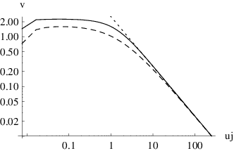
All curves show a linear behavior in the Mott phase, while in the superfluid regime our direct calculations produce the unphysical result of the visibility being larger than $1$. This is, again, due to fact that the above approximations are not appropriate in this parameter region. In the Mott region, on the other hand, all curves coincide and the linear dependence in $zJ/U$ is supported by experimental data [44, 11]. However, we note that the theoretical prefactor (40) turns out to be too small by a factor of about $2$. This discrepancy may arise from the approximation that our calculation is carried out for the homogeneous case, so the influence of the shell structure on the visibility is neglected. However, taking this effect into account should decrease the theoretical result even further, as the correlation function depends in a nonlinear way on the occupation number. In addition, we have also neglected the existence of superfluid regions between the Mott shells, but these are small and highly depleted deep in the Mott regime, so this effect should not play a decisive role.
Finally, we used the harmonic approximation for the Fourier transform of the Wannier functions so they cancelled in (36). As we show in Appendix A that the harmonic approximation can lead to large deviations, we investigate now its influence on the visibility.

We read off from Fig. 3, that the curve with the numerical Wannier envelope in the Mott regime no longer has a linear dependence on $J/U$ and lies above the experimental data. This discrepancy between our theoretical prediction for the visibility and the experimental findings can be explained as a temperature effect.
To this end we investigate at first the expanded result with the harmonic approximation (37), where it is sufficient to study the prefactor (38) for different chemical potentials, which corresponds to different occupation numbers.

We see in Fig. 4, that the thermal fluctuations slowly destroy the correlation and thus decrease the visibility. This qualitative finding within the harmonic approximation remains valid once the Wannier functions are calculated numerically.
Furthermore, we observe in Fig. 3 an increasing discrepancy between our theoretical prediction and the experimental findings for larger lattice depths. Note that a detailed analysis shows that this tendency is also present in the experimental data [11]. This discrepancy suggests an increasing temperature of the bosons in the lattice. This would support the assumption that the ramping of the optical lattice leads to an adiabatic heating of the Bose gas [32, 46]. In order to take into account this adiabatic heating one should determine the relation between temperature $T$ and the lattice depth $V_{0}$ from the condition that the entropy remains constant throughout the ramping process. This task is certainly a nontrivial one as this adiabatic calibration curve $T=T(V_{0})$ should be determined across the quantum phase transition. We expect that such a calibration curve could be deduced in a consistent way within the above mentioned effective action approach [45]. Once the inhomogeneity of the trap is included, it would be possible to get a visibility curve for constant entropy, which could then be used to determine the entropy present in the experiment and, finally, to determine the temperature for certain system parameters. One could then use remaining deviations from the theory to check if any non-adiabatic heating or non-equilibrium final states occur.

In this paper we calculated and analyzed the time-of-flight pictures and the resulting visibility for finite temperatures in a perturbative scheme for strong interactions going beyond the commonly used harmonic approximation. However, we did not achieve a full understanding of the experimental data, as the experimental situation is quite more complex than initially presumed. Comparing our theoretical calculations with experimental data suggested that the adiabatic heating process during the ramping of the optical lattice has to be taken into account. Thus, it becomes necessary to find a calibration curve, which allows to determine the temperature $T$ as a function of the potential depth $V_{0}$ for a given entropy.

We cordially thank Henrik Enoksen, Fabrice Gerbier, Robert Graham, Konstantin Krutitsky, Flavio Nogueira, Matthias Ohliger, and Ednilson Santos for stimulating discussions. Furthermore, we acknowledge financial support from the German Research Foundation (DFG) within the SFB/TR 12 Symmetries and Universality in Mesoscopic Systems.

References

- [1] M. Lewenstein, A. Sanpera, V. Ahufinger, B. Damski, A. Sen(De), and U. Sen, Adv. Phys. 56, 243 (2007).
- [2] I. Bloch, J. Dalibard, and W. Zwerger, Rev. Mod. Phys. 80, 885 (2008).
- [3] M. P. A. Fisher, P. B. Weichman, G. Grinstein, and D. S. Fisher, Phys. Rev. B 40, 546 (1989).
- [4] D. Jaksch, C. Bruder, J. I. Cirac, C. W. Gardiner, and P. Zoller, Phys. Rev. Lett. 81, 3108 (1998).
- [5] M. Greiner, O. Mandel, T. Esslinger, T. W. Hänsch, and I. Bloch, Nature 415, 39 (2002).
- [6] I. Bloch, Nature Phys. 1, 23 (2005).
- [7] W. Zwerger, Adv. Sol. State Phys. 44, 277 (2004).
- [8] D. Jaksch and P. Zoller, Ann. Phys. (New York) 315, 52 (2005).
- [9] T. Stöferle, H. Moritz, C. Schori, M. Köhl, and T. Esslinger, Phys. Rev. Lett. 92, 130403 (2004).
- [10] S. Fölling, A. Widera, T. Müller, F. Gerbier, and I. Bloch, Phys. Rev. Lett. 97, 060403 (2006).
- [11] F. Gerbier, A. Widera, S. Fölling, O. Mandel, T. Gericke, and I Bloch, Phys. Rev. A 72, 053606 (2005).
- [12] O. Morsch and M. Oberthaler, Rev. Mod. Phys 78, 179 (2006).
- [13] M. Greiner, O. Mandel, T.W. Hänsch, and I. Bloch, Nature, 419, 51 (2002).
- [14] C. Kollath, A. M. Läuchli, and E. Altman, Phys. Rev. Lett. 98, 180601 (2007).
- [15] U. R. Fischer and R. Schützhold, eprint: arXiv:0807.3627.
- [16] T. Rom, Th. Best, D. van Oosten, U. Schneider, S. Fölling, B. Paredes, and I. Bloch, Nature 444, 733 (2006).
- [17] K. Günter, T. Stöferle, H. Moritz, M Köhl, and T. Esslinger, Phys. Rev. Lett. 96, 180402 (2006).
- [18] S. Ospelkaus, C. Ospelkaus, O. Wille, M. Succo, P. Ernst, K. Sengstock, and K. Bongs, Phys. Rev. Lett. 96, 180403 (2006).
- [19] G. Refael and E. Demler, Phys. Rev. B 77, 144511 (2008).
- [20] C. Ospelkaus, S. Ospelkaus, L. Humbert, P. Ernst, K. Sengstock, and K. Bongs, Phys. Rev. Lett. 97, 120402 (2006).
- [21] B. Damski, L. Santos, E. Tiemann, M. Lewenstein, S. Kotochigova, P. Julienne, and P. Zoller, Phys. Rev. Lett. 90, 110401 (2003).
- [22] K. V. Krutitsky, A. Pelster, and R. Graham, New J. Phys. 8, 187 (2006).
- [23] K. V. Krutitsky, M. Thorwart, R. Egger, and R. Graham, Phys. Rev. A 77, 053609 (2008).
- [24] U. Bissbort and W. Hofstetter, eprint: arXiv:0804.0007.
- [25] J. J. Garcia-Ripoll and J. I. Cirac, Phil. Trans. R. Soc. 361, 1537 (2003).
- [26] A. Kay and K. Pachos, New J. Phys. 6, 126 (2004).
- [27] P. Treutlein, T. Steinmetz, Y. Colombe, B. Lev, P. Hommelhoff, J. Reichel, M. Greiner, O. Mandel, A. Widera, T. Rom, I. Bloch, T. W. Hänsch, Fortschr. Phys. 54, 702 (2006).
- [28] D. van Oosten, P. van der Straten, and H. T. C. Stoof, Phys. Rev. A 63, 053601 (2001).
- [29] J. K. Freericks and H. Monien, Phys. Rev. B 53, 2691 (1996).
- [30] B. Damski and J. Zakrzewski, Phys. Rev. A 74, 043609 (2006).
- [31] G. G. Batrouni, R. T. Scalettar, and G. T. Zimanyi, Phys. Rev. Lett. 65, 1765 (1990).
- [32] B. Capogrosso-Sansone, N. V. Prokof’ev, and B. V. Svistunov, Phys. Rev. B 75, 134302 (2007).
- [33] B. Capogrosso-Sansone, S. G. Söyler, N. V. Prokof’ev, and B. V. Svistunov, Phys. Rev. A 77, 015602 (2008).
- [34] E. F. A. dos Santos and A. Pelster, eprint: arXiv:0806.2812.
- [35] P. Buonsante and A. Vezzani, Phys. Rev. A 70, 033608 (2004).
- [36] F. Gerbier, Phys. Rev. Lett. 99, 120405 (2007).
- [37] M. Cramer, S. Ospelkaus, C. Ospelkaus, K. Bongs, K. Sengstock, and J. Eisert, Phys. Rev. Lett. 100, 140409 (2008).
- [38] K. Ziegler, Physica A 208, 177 (1994).
- [39] K. Ziegler, J. Low Temp. Phys. 126, 1431 (2002).
- [40] K. Ziegler, Las. Phys. 13, 587 (2003).
- [41] W. Zwerger, J. Optics B 5, S9 (2003).
- [42] A. Albus, F. Illuminati, and J. Eisert, Phys. Rev. A 68, 023606 (2003).
- [43] V. A. Kashurnikov, N. V. Prokof’ev, and B. V. Svistunov, Phys. Rev. A 66, 031601(R) (2002).
- [44] F. Gerbier, A. Widera, S. Fölling, O. Mandel, T. Gericke, and I Bloch, Phys. Rev. Lett. 95, 050404 (2005).
- [45] B. Bradlyn, E. F. A. dos Santos, and A. Pelster, arXiv:0809.0706.
- [46] T.-L. Ho and Q. Zhou Phys. Rev. Lett. 99, 120404 (2007).
- [47] K. Krutitsky, private communication.
- [48] P. B. Blakie and C. W. Clark, J. Phys. B 37, 1391 (2004).
- [49] F. Gerbier, S. Fölling, A. Widera, and I. Bloch, eprint: cond-mat/0701420.
- [50] G. G. Batrouni, V. Rousseau, R. T. Scalettar, M. Rigol, A. Muramatsu, P. J. H. Denteneer, and M. Troyer, Phys. Rev. Lett. 89, 117203 (2002).