跳到论文正文
W Papers独立论文阅读器 arXiv:0809.0706 论文正文 计算阅读时间 · 0%
引用这篇论文根据当前论文元数据生成,正式投稿前建议核对。


License: arXiv.org perpetual non-exclusive license
arXiv:0809.0706v3 [cond-mat.stat-mech] 20 Jan 2009

Effective Action Approach for Quantum Phase Transitions in Bosonic Lattices

Barry Bradlyn Affiliation: Department of Physics, Massachusetts Institute of Technology, Cambridge, Massachusetts 02139, USA Email: bbradlyn@mit.edu    Francisco Ednilson A. dos Santos Affiliation: Institut für Theoretische Physik, Freie Universität Berlin, Arnimallee 14, 14195 Berlin, Germany Email: santos@physik.fu-berlin.de    Axel Pelster Affiliation: Fachbereich Physik, Universität Duisburg-Essen, Campus Duisburg, Lotharstrasse 1, 47048 Duisburg, Germany Email: axel.pelster@uni-duisburg-essen.de
August 24, 2026
Abstract

Based on standard field-theoretic considerations, we develop an effective action approach for investigating quantum phase transitions in lattice Bose systems at arbitrary temperature. We begin by adding to the Hamiltonian of interest a symmetry breaking source term. Using time-dependent perturbation theory, we then expand the grand-canonical free energy as a double power series in both the tunneling and the source term. From here, an order parameter field is introduced in the standard way, and the underlying effective action is derived via a Legendre transformation. Determining the Ginzburg-Landau expansion to first order in the tunneling term, expressions for the Mott insulator–superfluid phase boundary, condensate density, average particle number, and compressibility are derived and analyzed in detail. Additionally, excitation spectra in the ordered phase are found by considering both longitudinal and transverse variations of the order parameter. Finally, these results are applied to the concrete case of the Bose-Hubbard Hamiltonian on a three dimensional cubic lattice, and compared with the corresponding results from mean-field theory. Although both approaches yield the same Mott insulator - superfluid phase boundary to first order in the tunneling, the predictions of our effective action theory turn out to be superior to the mean-field results deeper into the superfluid phase.

I Introduction

Recent developments in the field of dilute ultracold quantum gasses [1, 2, 3, 4, 5] have led to the experimental investigation of atoms in periodic potentials [6]. They are a fascinating new generation of many-particle quantum systems as they allow for the study of a variety of solid-state phenomena under perfectly controlled conditions [4, 6, 7, 8, 9, 10, 11, 12]. For instance, Bosonic lattice systems show a quantum phase transition for varying lattice depths. In deep lattices the tunneling between lattice sites is suppressed, and a Mott insulating state forms with a fixed number of Bosons residing on each lattice site. For shallow lattices, however, the dominance of inter-site tunneling allows for Bosons to coherently spread over the whole lattice, forming a superfluid. The occurrence of such a quantum phase transition between a Mott insulator and a superfluid is observable, for instance, in time-of-flight absorption pictures taken after switching off the lattice potential. They image momentum distributions integrated along one axis, and therefore by Heisenberg’s uncertainty principle give information about the corresponding spacial distributions. Thus, the localization of atoms in the Mott phase results in diffuse absorption pictures, while the delocalized superfluid phase gives rise to Bragg-like interference patterns.

The theoretical analysis of this quantum phase transition is usually based on the Bose-Hubbard model Hamiltonian [13, 14, 15, 16],

H^BH=∑i[12​U​a^i†​a^i​(a^i†​a^i−1)−μ​a^i†​a^i]−t​∑⟨i,j⟩a^i†​a^j,\hat{H}_{\mathrm{BH}}=\sum_{i}{\left[\frac{1}{2}U\hat{a}^{{\dagger}}_{i}\hat{a}_{i}\Big(\hat{a}^{{\dagger}}_{i}\hat{a}_{i}-1\Big)-\mu\hat{a}^{{\dagger}}_{i}\hat{a}_{i}\right]}-t\sum_{\left<i,j\right>}{\hat{a}^{{\dagger}}_{i}\hat{a}_{j}}, (1)

where a^i\hat{a}_{i} and a^i†\hat{a}^{{\dagger}}_{i} are Bosonic annihilation and creation operators, μ\mu is the chemical potential, and ⟨i,j⟩\left<i,j\right> signifies a sum over nearest neighbor sites ii and jj. Additionally, UU parameterizes the on-site interaction energy between two atoms at a given site, and tt characterizes the kinetic energy, in this case given by the tunneling of an atom between two neighboring lattice sites. The quartic on-site coupling term, however, makes an exact diagonalization of (1) impossible. Thus, while Monte-Carlo simulations have proven fruitful for obtaining numerical results [17, 18, 19], analytic descriptions of Bosonic lattices near the quantum phase boundary have so far been typically limited to mean-field [13, 15] or strong-coupling approximations [20, 21]. Currently, the most precise analytic result for the whole Mott insulator-superfluid phase diagram in a three dimensional cubic lattice at zero temperature is found in Ref. [22]. Therein, a Landau expansion for an effective potential with a spatially and temporally global order parameter is derived. In this paper, we generalize the results of Ref. [22] by allowing for a spacially and temporally varying order parameter, thus determining a Ginzburg-Landau expansion for the effective action. This allows us to obtain an approximate analytic description of Bosonic lattice systems near the quantum phase boundary.

To this end we proceed as follows. In Section II, we consider a very general type of Hamiltonian consisting of an arbitrary on-site interaction and an arbitrary tunneling term, of which the Bose-Hubbard Hamiltonian is a special case, and determine the grand-canonical free energy to first order in the tunneling term. This tunneling approximation is motivated by the fact that in three dimensions, the Mott insulator-superfluid quantum phase transition is observed to occur for small values of t/U{t}/{U} (note that the tunneling expansion is related to the random-walk expansion of Refs. [23, 24, 25]). Next, in Section III we introduce an order parameter field and derive a Ginzburg-Landau expansion of the effective action, allowing for the computation of physical quantities near the phase boundary in both the Mott insulator and the superfluid phase. Sections IV and V present predictions of our effective-action theory for both static homogeneous and spatio-temporally varying order parameter fields, including expressions for the particle density, the compressibility, the superfluid density, and the excitation spectra. Finally, in Section VI, we specify our results to the Bose-Hubbard Hamiltonian, and compare them to the predictions of the standard mean-field theory. Although both approaches yield the same approximation for the location of the phase boundary, our effective action approach turns out to be superior to the mean-field theory for the following reasons. First, we demonstrate that the effective action approach leads to qualitatively better results deeper into the superfluid phase. Secondly, in contrast to the mean-field approximation, the effective action approach can be systematically extended to higher orders in the tunneling parameter in order to quantitatively improve the results, as has already been demonstrated for the case of the effective potential in Ref. [22].

II Grand-Canonical Free Energy

We consider Bosons on a background lattice with lattice sites denoted by ii. Suppose they are described by a Hamiltonian of the form

H^=H^0+H^1,\hat{H}=\hat{H}_{0}+\hat{H}_{1}, (2)

which depends on Bosonic creation and annihilation operators a^i†\hat{a}^{{\dagger}}_{i} and a^i\hat{a}_{i} obeying the standard commutation relations

[a^i,a^j]=[a^i†,a^j†]=0,[a^i,a^j†]=δi​j.\Big[\hat{a}_{i},\hat{a}_{j}\Big]=\left[\hat{a}^{{\dagger}}_{i},\hat{a}^{{\dagger}}_{j}\right]=0,\,\,\,\left[\hat{a}_{i},\hat{a}^{{\dagger}}_{j}\right]=\delta_{ij}. (3)

We assume that H^0\hat{H}_{0} is a sum of local terms each diagonal in the occupation number basis, i.e.

H^0=∑ifi​(a^i†​a^i)\hat{H}_{0}=\sum_{i}{f_{i}(\hat{a}^{\dagger}_{i}\hat{a}_{i})} (4)

so its energy eigenvalues are given by

E{ni}=∑ifi​(ni).E_{\{n_{i}\}}=\sum_{i}f_{i}(n_{i}). (5)

As we will be working grand-canonically, we stipulate that the terms fi​(a^i†​a^i)f_{i}(\hat{a}^{\dagger}_{i}\hat{a}_{i}) include the usual −μ​a^i†​a^i-\mu\hat{a}^{{\dagger}}_{i}\hat{a}_{i} dependence on the chemical potential μ\mu. Also, we make the simplifying assumption that H^1\hat{H}_{1} is only a two-Boson hopping term

H^1\displaystyle\hat{H}_{1} =−∑i​jti​ja^†ia^j\displaystyle=-\sum_{ij}{t_{ij}\hat{a}^{\dagger}_{i}\hat{a}_{j}} (6)

with ti​jt_{ij} symmetric in ii and jj and ti​i=0t_{ii}=0. As with the Bose-Hubbard model (1), H^0\hat{H}_{0} in Eq. (4) describes the Bosonic on-site interaction, while H^1\hat{H}_{1} in Eq. (6) incorporates the tunneling of Bosons between lattice sites. Note, however, that Eq. (2) with Eqs. (4) and (6) covers a significantly more general scenario than the Bose-Hubbard model. The on-site interaction in the Bose-Hubbard model (1) is a two-Boson term with a global interaction strength, but in Eq. (4), however, we have allowed for the on-site interaction of any finite number of Bosons. In addition, we have allowed the Hamiltonian to vary between lattice sites. Thus, our model is also capable of describing on-site disorder, which may arise from a local chemical potential, or from a local interaction [4, 13, 26]. Furthermore, Eq. (6) contains not only the tunneling of Bosons between nearest neighbor sites as in Eq. (2), but also between arbitrarily distant sites.

As we are ultimately interested in investigating quantum phase transitions, we follow general field-theoretic considerations and add source terms to the Hamiltonian (2) in order to explicitly break any global symmetries [27, 28]

H^1→H^1′=−∑i​jti​ja^i†a^j+∑i[ji(τ)a^i†+ji∗(τ)a^i].\displaystyle\hat{H}_{1}\rightarrow\hat{H}_{1}^{\prime}=-\sum_{ij}{t_{ij}\hat{a}^{\dagger}_{i}\hat{a}_{j}}+\sum_{i}{\left[j_{i}(\tau)\hat{a}^{\dagger}_{i}+j^{*}_{i}(\tau)\hat{a}_{i}\right]}. (7)

Since the source currents ji​(τ),ji∗​(τ)j_{i}(\tau),j^{*}_{i}(\tau) depend explicitly upon the imaginary time variable τ\tau, standard time-dependent perturbation theory may be used to find a perturbative expression for the grand-canonical free energy. To do this, we switch to the imaginary-time Dirac interaction picture [29], with operators given by

O^D​(τ)=eτ​H^0​O^​e−τ​H^0,\hat{O}_{\mathrm{D}}(\tau)=e^{\tau\hat{H}_{0}}\hat{O}e^{-\tau\hat{H}_{0}}, (8)

where we have set ℏ=1\hbar=1. In this representation, the Schrödinger initial value problem for the time-evolution operator takes the form

dd​τ​U^D​(τ,τ0)\displaystyle\frac{d}{d\tau}\hat{U}_{\mathrm{D}}(\tau,\tau_{0}) =−H^1​D′​(τ)​U^D​(τ,τ0),\displaystyle=-\hat{H}_{1\mathrm{D}}^{\prime}(\tau)\hat{U}_{\mathrm{D}}(\tau,\tau_{0}), (9)
U^D​(τ0,τ0)\displaystyle\hat{U}_{\mathrm{D}}(\tau_{0},\tau_{0}) =1.\displaystyle=1. (10)

This is solved by the Dyson expansion

U^D​(τ,τ0)\displaystyle\hat{U}_{\mathrm{D}}(\tau,\tau_{0}) =1+∑n=1∞U^D(n)​(τ,τ0),\displaystyle=1+\sum_{n=1}^{\infty}{\hat{U}_{\mathrm{D}}^{(n)}(\tau,\tau_{0})}, (11)
U^D(n)​(τ,τ0)\displaystyle\hat{U}_{\mathrm{D}}^{(n)}(\tau,\tau_{0}) =(−1)nn!​∫τ0τd​τ1​∫τ0τd​τ2​…​∫τ0τd​τn​T^​[H^1​D′​(τ1)​H^1​D′​(τ2)​…​H^1​D′​(τn)],\displaystyle=\frac{(-1)^{n}}{n!}\int_{\tau_{0}}^{\tau}{\!\!\!\!\mathrm{d}\tau_{1}}\int_{\tau_{0}}^{\tau}{\!\!\!\!\mathrm{d}\tau_{2}}\dots\int_{\tau_{0}}^{\tau}{\!\!\!\!\mathrm{d}\tau_{n}\hat{T}\left[\hat{H}_{1\mathrm{D}}^{\prime}(\tau_{1})\hat{H}_{1\mathrm{D}}^{\prime}(\tau_{2})\dots\hat{H}_{1\mathrm{D}}^{\prime}(\tau_{n})\right]}, (12)

where T^\hat{T} is the standard imaginary-time ordering operator. The grand-canonical partition function for the system is defined as

𝒵=tr{T^e−∫0βdτH^(τ)},\mathcal{Z}=\mathrm{tr}\left\{\hat{T}e^{-\int_{0}^{\beta}\mathrm{d}\tau\hat{H}(\tau)}\right\}, (13)

which can be rewritten as

𝒵=tr⁡{e−β​H^0​U^D​(β,0)}.\mathcal{Z}=\mathrm{tr}\left\{e^{-\beta\hat{H}_{0}}\hat{U}_{\mathrm{D}}(\beta,0)\right\}. (14)

This gives the partition function 𝒵\mathcal{Z} as a functional of the currents. For brevity, we shall - in cases where no confusion may arise - suppress the arguments of functionals. Thus, by substituting Eqs. (11) and (12) into Eq. (14), we obtain

𝒵\displaystyle\mathcal{Z} =𝒵(0)+∑n=1∞𝒵(n),\displaystyle=\mathcal{Z}^{(0)}+\sum_{n=1}^{\infty}{\mathcal{Z}^{(n)}}, (15)
𝒵(n)\displaystyle\mathcal{Z}^{(n)} =𝒵(0)​(−1)nn!​∫0βd​τ1​∫0βd​τ2​…​∫0βd​τn​⟨T^​[H^1​D′​(τ1)​H^1​D′​(τ2)​…​H^1​D′​(τn)]⟩0,\displaystyle=\mathcal{Z}^{(0)}\frac{(-1)^{n}}{n!}\int_{0}^{\beta}{\!\!\!\!\mathrm{d}\tau_{1}}\int_{0}^{\beta}{\!\!\!\!\mathrm{d}\tau_{2}}\dots\int_{0}^{\beta}{\!\!\!\!\mathrm{d}\tau_{n}\left<\hat{T}\left[\hat{H}_{1\mathrm{D}}^{\prime}(\tau_{1})\hat{H}_{1\mathrm{D}}^{\prime}(\tau_{2})\dots\hat{H}_{1\mathrm{D}}^{\prime}(\tau_{n})\right]\right>_{0}}, (16)

where

𝒵i(0)=tr⁡{e−β​H^0}=∏i∑n=0∞e−β​fi​(n)\mathcal{Z}^{(0)}_{i}=\mathrm{tr}\{e^{-\beta\hat{H}_{0}}\}=\prod_{i}\sum_{n=0}^{\infty}e^{-\beta f_{i}(n)} (17)

is the partition function of the unperturbed system, and

<∙>0=1𝒵(0)tr{∙e−β​H^0}<\bullet>_{0}=\frac{1}{\mathcal{Z}^{(0)}}\mathrm{tr}\left\{\bullet\,e^{-\beta\hat{H}_{0}}\right\} (18)

represents the thermal average with respect to the unperturbed Hamiltonian H^0\hat{H}_{0}. This can be expressed more compactly as

𝒵=𝒵(0)⟨T^exp(−∫0βdτH^1​D′(τ))⟩0.\mathcal{Z}=\mathcal{Z}^{(0)}\left<\hat{T}\exp\left(-\int_{0}^{\beta}{\!\!\!\!\mathrm{d}\tau\hat{H}^{\prime}_{1\mathrm{D}}(\tau)}\right)\right>_{0}. (19)

Inserting the explicit form of H^1​D′​(τ)\hat{H}_{1\mathrm{D}}^{\prime}(\tau) from Eqs. (7) and (8), we see that the expectation values appearing in Eq. (16) can be expanded in terms of Green’s functions of the unperturbed system. Furthermore, since the grand-canonical free energy is given as a logarithm of the partition function

ℱ=−1β​log⁡𝒵,\mathcal{F}=-\frac{1}{\beta}\log\mathcal{Z}, (20)

the Linked Cluster Theorem [30] tells us that ℱ\mathcal{F} can be expanded diagrammatically in terms of cumulants defined as

C2​n(0)(i1′,τ1′;…;in′,τn′|i1,τ1;…;in,τn)=δ2​n​C0(0)​[j,j∗]δ​ji1′​(τ1′)​…​δ​jin′​(τn′)​δ​ji1∗​(τ1)​…​δ​jin∗​(τn)|j=j∗=0,\displaystyle C_{2n}^{(0)}(i_{1}^{\prime},\tau_{1}^{\prime};\dots;i_{n}^{\prime},\tau_{n}^{\prime}|i_{1},\tau_{1};\dots;i_{n},\tau_{n})=\left.\frac{\delta^{2n}C_{0}^{(0)}[j,j^{*}]}{\delta j_{i^{\prime}_{1}}(\tau^{\prime}_{1})\dots\delta j_{i^{\prime}_{n}}(\tau^{\prime}_{n})\delta j^{*}_{i_{1}}(\tau_{1})\dots\delta j^{*}_{i_{n}}(\tau_{n})}\right|_{j=j^{*}=0}, (21)

with the generating functional

C0(0)​[j,j∗]=log⁡𝒵𝒵(0)|ti​j≡0=log⁡⟨T^​exp⁡{−(∑i∫0βd​τ​[ji​(τ)​a^i†​(τ)+ji∗​(τ)​a^i​(τ)])}⟩0,\displaystyle C_{0}^{(0)}[j,j^{*}]=\log\left.\frac{\mathcal{Z}}{\mathcal{Z}^{(0)}}\right|_{t_{ij}\equiv 0}=\log{\left<\hat{T}\exp{\left\{-\left(\sum_{i}{\int_{0}^{\beta}{\mathrm{d}\tau\left[j_{i}(\tau)\hat{a}^{{\dagger}}_{i}(\tau)+j_{i}^{*}(\tau)\hat{a}_{i}(\tau)\right]}}\right)\right\}}\right>_{0}}, (22)

with only contributions from connected diagrams [31]. Note that this approach, rather than a decomposition of the Green’s functions via Wick’s theorem, must be used in our case as H^0\hat{H}_{0} is not necessarily quadratic in the creation and annihilation operators. Because H^0\hat{H}_{0} is local according to Eq. (4), the average in Eq. (22) factors into independent averages for each lattice site. It follows that C0(0)​[j,j∗]C_{0}^{(0)}[j,j^{*}] is a sum of local quantities, and thus the cumulants C2​n(0)(i1′,τ1′;…;in′,τn′|i1,τ1;…;in,τn)C_{2n}^{(0)}(i_{1}^{\prime},\tau_{1}^{\prime};\dots;i_{n}^{\prime},\tau_{n}^{\prime}|i_{1},\tau_{1};\dots;i_{n},\tau_{n}) vanish unless all site indices are equal. With this, we can write

C2​n(0)(i1′,τ1′;…;in′,τn′|i1,τ1;…;in,τn)=C2​n(0)i1(τ1′,…,τn′|τ1,…,τn)∏n,mδin′,im,C_{2n}^{(0)}(i_{1}^{\prime},\tau_{1}^{\prime};\dots;i_{n}^{\prime},\tau_{n}^{\prime}|i_{1},\tau_{1};\dots;i_{n},\tau_{n})={{}_{i_{1}}C}_{2n}^{(0)}(\tau_{1}^{\prime},\dots,\tau_{n}^{\prime}|\tau_{1},\dots,\tau_{n})\prod_{n,m}{\delta_{i^{\prime}_{n},i_{m}}}, (23)

so that it only remains to determine the local quantities C2​n(0)i(τ1′,…,τn′|τ1,…,τn){}_{i}C_{2n}^{(0)}(\tau_{1}^{\prime},\dots,\tau_{n}^{\prime}|\tau_{1},\dots,\tau_{n}). Using the definitions (21) and (22), we find that

C2(0)i(τ1|τ2)=⟨T^[a^i†(τ1)a^i(τ2)]⟩0=G(0)(i,τ1|i,τ2),{}_{i}C^{(0)}_{2}(\tau_{1}|\tau_{2})=\left<\hat{T}\left[\hat{a}^{{\dagger}}_{i}(\tau_{1})\hat{a}_{i}(\tau_{2})\right]\right>_{0}=G^{(0)}(i,\tau_{1}|i,\tau_{2}), (24)

where G(0)(i,τ1|j,τ2)=δi​jG(0)(i,τ1|i,τ2)G^{(0)}(i,\tau_{1}|j,\tau_{2})=\delta_{ij}G^{(0)}(i,\tau_{1}|i,\tau_{2}) is the imaginary-time Green’s function of the unperturbed system. Similarly,

C4(0)i(τ1,τ2|τ3,τ4)={}_{i}C^{(0)}_{4}(\tau_{1},\tau_{2}|\tau_{3},\tau_{4})= ⟨T^​[a^i†​(τ1)​a^i†​(τ2)​a^i​(τ3)​a^i​(τ4)]⟩0\displaystyle\left<\hat{T}\left[\hat{a}^{{\dagger}}_{i}(\tau_{1})\hat{a}^{{\dagger}}_{i}(\tau_{2})\hat{a}_{i}(\tau_{3})\hat{a}_{i}(\tau_{4})\right]\right>_{0}
−C2(0)i(τ1|τ3)iC2(0)(τ2|τ4)−iC2(0)(τ1|τ4)iC2(0)(τ2|τ3).\displaystyle-{{}_{i}C}^{(0)}_{2}(\tau_{1}|\tau_{3})_{i}C^{(0)}_{2}(\tau_{2}|\tau_{4})-_{i}C^{(0)}_{2}(\tau_{1}|\tau_{4})_{i}C^{(0)}_{2}(\tau_{2}|\tau_{3}). (25)

Note that local the quantity C4(0)i(τ1,τ2|τ3,τ4){}_{i}C^{(0)}_{4}(\tau_{1},\tau_{2}|\tau_{3},\tau_{4}) is symmetric under both the exchanges τ1↔τ2\tau_{1}\leftrightarrow\tau_{2} and τ3↔τ4\tau_{3}\leftrightarrow\tau_{4}.

Because each power of the tunneling parameter ti​jt_{ij} is associated with a creation operator and an annihilation operator, and each power of ji​(τ)j_{i}(\tau) (ji∗​(τ)j^{*}_{i}(\tau)) is associated with one creation (annihilation) operator, we can construct the connected diagrams which contribute to ℱ\mathcal{F} according to the following rules [32]:

  1. 1.

    Each vertex with nn lines entering and nn lines exiting corresponds to a 2​n2n-th order cumulant C(0)2​ni{}_{i}C_{2n}^{(0)}.

  2. 2.

    Draw all topologically inequivalent connected diagrams.

  3. 3.

    Label each vertex with a site index, and each line with an imaginary-time variable.

  4. 4.

    Each internal line is associated with a factor of ti​jt_{ij}.

  5. 5.

    Each incoming (outgoing) external line is associated with a factor of ji​(τ)j_{i}(\tau) (ji∗​(τ)j^{*}_{i}(\tau)).

  6. 6.

    Multiply by the multiplicity and divide by the symmetry factor.

  7. 7.

    Integrate over all internal time variables.

Each diagram is then multiplied by the appropriate factors of ji​(τ)j_{i}(\tau), ji∗​(τ)j_{i}^{*}(\tau), and ti​jt_{ij}, and all spacetime variables are integrated. Since H^0\hat{H}_{0} in Eq. (4) is diagonal in the occupation number basis and local, there can be no contributions from diagrams with one line. Thus, to first order in the tunneling ti​jt_{ij} and fourth order in the currents ji​(τ)j_{i}(\tau) we find

ℱ=\displaystyle\mathcal{F}= F0−1β∑i{∫0βdτ1∫0βdτ2[a2(0)(i,τ1|i,τ2)ji(τ1)ji∗(τ2)+∑ja2(1)(i,τ1|j,τ2)ti​jji(τ1)jj∗(τ2)]\displaystyle F_{0}-\frac{1}{\beta}\sum_{i}{}\left\{\int_{0}^{\beta}{\!\!\!\!\mathrm{d}\tau_{1}}\int_{0}^{\beta}{\!\!\!\!\mathrm{d}\tau_{2}\left[a_{2}^{(0)}(i,\tau_{1}|i,\tau_{2})j_{i}(\tau_{1})j^{*}_{i}(\tau_{2})+\sum_{j}{a_{2}^{(1)}(i,\tau_{1}|j,\tau_{2})t_{ij}j_{i}(\tau_{1})j^{*}_{j}(\tau_{2})}\right]}\right.
+14∫0βdτ1∫0βdτ2∫0βdτ3∫0βdτ4a4(0)(i,τ1;i,τ2|i,τ3;i,τ4)ji(τ1)ji(τ2)ji∗(τ3)ji∗(τ4)\displaystyle+\frac{1}{4}\int_{0}^{\beta}{\!\!\!\!\mathrm{d}\tau_{1}}\!\!\int_{0}^{\beta}{\!\!\!\!\mathrm{d}\tau_{2}}\!\!\int_{0}^{\beta}{\!\!\!\!\mathrm{d}\tau_{3}}\!\!\int_{0}^{\beta}{\!\!\!\!\mathrm{d}\tau_{4}\,a_{4}^{(0)}(i,\tau_{1};i,\tau_{2}|i,\tau_{3};i,\tau_{4})j_{i}(\tau_{1})j_{i}(\tau_{2})j^{*}_{i}(\tau_{3})j^{*}_{i}(\tau_{4})}
+12∫0βdτ1∫0βdτ2∫0βdτ3∫0βdτ4∑jti​j[a4(1)(i,τ1;i,τ2|j,τ3;i,τ4)ji(τ1)ji(τ2)jj∗(τ3)ji∗(τ4)\displaystyle+\frac{1}{2}\left.\int_{0}^{\beta}{\!\!\!\!\mathrm{d}\tau_{1}}\!\!\int_{0}^{\beta}{\!\!\!\!\mathrm{d}\tau_{2}}\!\!\int_{0}^{\beta}{\!\!\!\!\mathrm{d}\tau_{3}}\!\!\int_{0}^{\beta}{\!\!\!\!\mathrm{d}\tau_{4}}\sum_{j}\,t_{ij}\left[a_{4}^{(1)}(i,\tau_{1};i,\tau_{2}|j,\tau_{3};i,\tau_{4})j_{i}(\tau_{1})j_{i}(\tau_{2})j^{*}_{j}(\tau_{3})j^{*}_{i}(\tau_{4})\right.\right.
+a4(1)(i,τ1;j,τ2|i,τ3;i,τ4)ji(τ1)jj(τ2)ji∗(τ3)ji∗(τ4)]},\displaystyle+\left.\left.a_{4}^{(1)}(i,\tau_{1};j,\tau_{2}|i,\tau_{3};i,\tau_{4})j_{i}(\tau_{1})j_{j}(\tau_{2})j^{*}_{i}(\tau_{3})j^{*}_{i}(\tau_{4})\right]\right\}, (26)

where

F0=−1βlog𝒵(0)=−1β∑ilog{∑n=0∞e−β​fi​(n)}F_{0}=-\frac{1}{\beta}\log\mathcal{Z}^{(0)}=-\frac{1}{\beta}\sum_{i}\log\left\{\sum_{n=0}^{\infty}e^{-\beta f_{i}(n)}\right\} (27)

is the grand-canonical free energy of the unperturbed system, and the respective coefficients a2​na_{2n} are given by the following diagrams and expressions:

a2(0)(i,τ1|i,τ2)\displaystyle a_{2}^{(0)}(i,\tau_{1}|i,\tau_{2}) =††feynman-diagram: (Feynman diagram, (x2)=C2(0)i(τ1|τ2),\displaystyle=\;\;\;\;\;\begin{fmffile}\begin{fmfgraph*}{2}5,1) \end{fmfgraph*}\end{fmffile}\;\;\;\;\;={{}_{i}C}_{2}^{(0)}(\tau_{1}|\tau_{2}), (28)
a2(1)(i,τ1|j,τ2)\displaystyle a_{2}^{(1)}(i,\tau_{1}|j,\tau_{2}) =††feynman-diagram: (Feynman diagram, (x2)=∫0βdτC2(0)i(τ1|τ)C2(0)j(τ|τ2),\displaystyle=\;\;\;\;\;\begin{fmffile}\begin{fmfgraph*}{2}5,1) \end{fmfgraph*}\end{fmffile}\;\;\;\;\;=\int_{0}^{\beta}{\mathrm{d}\tau{{}_{i}C}_{2}^{(0)}(\tau_{1}|\tau){{}_{j}C}_{2}^{(0)}(\tau|\tau_{2})}, (29)
a4(0)(i,τ1;i,τ2|i,τ3;i,τ4)\displaystyle a_{4}^{(0)}(i,\tau_{1};i,\tau_{2}|i,\tau_{3};i,\tau_{4}) =††feynman-diagram: (Feynman diagram, (x2)=C4(0)i(τ1,τ2|τ3,τ4),\displaystyle=\;\;\;\;\;\begin{fmffile}\begin{fmfgraph*}{2}5,10) \end{fmfgraph*}\end{fmffile}\;\;\;\;\;={{}_{i}C}_{4}^{(0)}(\tau_{1},\tau_{2}|\tau_{3},\tau_{4}), (30)
a4(1)(i,τ1;i,τ2|j,τ3;i,τ4)\displaystyle a_{4}^{(1)}(i,\tau_{1};i,\tau_{2}|j,\tau_{3};i,\tau_{4}) =††feynman-diagram: (Feynman diagram, (x2)=∫0βdτC4(0)i(τ1,τ2|τ,τ4)C2(0)j(τ|τ3).\displaystyle=\;\;\;\;\;\begin{fmffile}\begin{fmfgraph*}{2}5,10) \end{fmfgraph*}\end{fmffile}\;\;\;\;\;=\int_{0}^{\beta}{\mathrm{d}\tau{{}_{i}C}_{4}^{(0)}(\tau_{1},\tau_{2}|\tau,\tau_{4}){{}_{j}C}_{2}^{(0)}(\tau|\tau_{3})}. (31)

In the next section, we will see how this expansion (26) of the grand-canonical free energy leads to the Ginzburg-Landau expansion of the effective action to first order in ti​jt_{ij}.

At this point, it is also worth making some observations about the two-particle Green’s function G(i,τ1|j,τ2)G(i,\tau_{1}|j,\tau_{2}), defined in the standard way as

G(i,τ1|j,τ2)=⟨T^[a^i†(τ1)a^j(τ2)]⟩=−βδ2​ℱδ​ji​(τ1)​δ​jj∗​(τ2)=1𝒵tr{e−β​H^0δ2​U^D​(β,0)δ​ji​(τ1)​δ​jj∗​(τ2)}.G(i,\tau_{1}|j,\tau_{2})=\left<\hat{T}\left[\hat{a}^{{\dagger}}_{i}(\tau_{1})\hat{a}_{j}(\tau_{2})\right]\right>=-\beta\frac{\delta^{2}\mathcal{F}}{\delta j_{i}(\tau_{1})\delta j^{*}_{j}(\tau_{2})}=\frac{1}{\mathcal{Z}}\mathrm{tr}\left\{e^{-\beta\hat{H}_{0}}\frac{\delta^{2}\hat{U}_{\mathrm{D}}(\beta,0)}{\delta j_{i}(\tau_{1})\delta j^{*}_{j}(\tau_{2})}\right\}. (32)

This quantity can also be expanded diagrammatically in terms of cumulants, provided we realize that the effect of the prefactor 1/𝒵1/{\mathcal{Z}} in Eq. (32) is simply to cancel all disconnected diagrams [29], ensuring that the only diagrams that contribute are connected diagrams with two external lines [31, 32]. Thus, there is a natural correspondence between the Green’s function and the coefficients a2(n)a_{2}^{(n)} defined above:

G(i,τ1|j,τ2)\displaystyle G(i,\tau_{1}|j,\tau_{2}) =G(0)(i,τ1|j,τ2)+G(1)(i,τ1|j,τ2)+…\displaystyle=G^{(0)}(i,\tau_{1}|j,\tau_{2})+G^{(1)}(i,\tau_{1}|j,\tau_{2})+\dots
=δi​ja2(0)(i,τ1|i,τ2)+a2(1)(i,τ1|j,τ2)+….\displaystyle=\delta_{ij}a_{2}^{(0)}(i,\tau_{1}|i,\tau_{2})+a_{2}^{(1)}(i,\tau_{1}|j,\tau_{2})+\dots. (33)

III Effective Action

Evaluation of the diagrams shown in Eqs. (29) and (31) involve integration over the time variable associated with the internal line. Thus, their evaluation can be simplified by transforming to Matsubara space, where these integrals amount to simple multiplication. We use the following convention for the forward and inverse Matsubara transformations

g⁡(ωm)\displaystyle g(\omega_{m}) =1β​∫0βd​τ​ei​ωm​τ​g​(τ),\displaystyle=\frac{1}{\sqrt{\beta}}\int_{0}^{\beta}{\!\!\!\!\mathrm{d}\tau\,e^{i\omega_{m}\tau}g(\tau)}, (34)
g⁡(τ)\displaystyle g(\tau) =1β​∑m=−∞∞g⁡(ωm)​e−i​ωm​τ,\displaystyle=\frac{1}{\sqrt{\beta}}\sum_{m=-\infty}^{\infty}{g(\omega_{m})e^{-i\omega_{m}\tau}}, (35)

with the Matsubara frequencies

ωm\displaystyle\omega_{m} =2​π​mβ,m∈ℤ.\displaystyle=\frac{2\pi m}{\beta}\,\,\,,\,\,\,m\in\mathbb{Z}. (36)

Since the unperturbed Hamiltonian (4) is time-translation invariant, it follows from Eqs. (21) and (22) that the cumulants - and thus the functions a2​na_{2n} - must depend on time-differences only. In terms of Matsubara frequencies, this implies that one of the frequency variables is restricted by a delta function, i.e. we have

a2(0)(i,ωm​1|i,ωm​2)\displaystyle a_{2}^{(0)}(i,\omega_{m1}|i,\omega_{m2}) =a2(0)​(i,ωm​1)​δωm​1,ωm​2,\displaystyle=a_{2}^{(0)}(i,\omega_{m1})\delta_{\omega_{m1},\omega_{m2}}, (37)
a4(0)(i,ωm​1;i,ωm​2|i,ωm​3;i,ωm​4)\displaystyle a_{4}^{(0)}(i,\omega_{m1};i,\omega_{m2}|i,\omega_{m3};i,\omega_{m4}) =a4(0)(i,ωm​1;i,ωm​2|i,ωm​4)δωm​1+ωm​2,ωm​3+ωm​4.\displaystyle=a_{4}^{(0)}(i,\omega_{m1};i,\omega_{m2}|i,\omega_{m4})\delta_{\omega_{m1}+\omega_{m2},\omega_{m3}+\omega_{m4}}. (38)

Using this frequency conservation, we find from Eq. (29)

a2(1)(i,ωm​1|j,ωm​2)\displaystyle a_{2}^{(1)}(i,\omega_{m1}|j,\omega_{m2}) =a2(0)​(i,ωm​1)​a2(0)​(j,ωm​1)​δωm​1,ωm​2,\displaystyle=a_{2}^{(0)}(i,\omega_{m1})a_{2}^{(0)}(j,\omega_{m1})\delta_{\omega_{m1},\omega_{m2}}, (39)

and correspondingly Eq. (31) implies

a4(1)(i,ωm​1;i,ωm​2|j,ωm​3;i,ωm​4)\displaystyle a_{4}^{(1)}(i,\omega_{m1};i,\omega_{m2}|j,\omega_{m3};i,\omega_{m4}) =a4(0)(i,ωm​1;i,ωm​2|i,ωm​4)a2(0)(j,ωm​3)δωm​1+ωm​2,ωm​3+ωm​4.\displaystyle=a_{4}^{(0)}(i,\omega_{m1};i,\omega_{m2}|i,\omega_{m4})a_{2}^{(0)}(j,\omega_{m3})\delta_{\omega_{m1}+\omega_{m2},\omega_{m3}+\omega_{m4}}. (40)

Thus, the first order corrections to the functions a2​na_{2n} can be expressed entirely in terms of a2(0)a_{2}^{(0)} and the corresponding zeroth order terms. Using the expressions (28) and (30), along with the definitions (24) and (25), we find that these two coefficients are explicitly given by

a2(0)​(i,ωm)=\displaystyle a_{2}^{(0)}(i,\omega_{m})= 1𝒵(0)​∑n=0∞e−β​fi​(n)\displaystyle\frac{1}{\mathcal{Z}^{(0)}}\sum_{n=0}^{\infty}e^{-\beta f_{i}(n)}
×[n+1fi​(n+1)−fi​(n)−i​ωm−nfi​(n)−fi​(n−1)−i​ωm],\displaystyle\times\left[\frac{n+1}{f_{i}(n+1)-f_{i}(n)-i\omega_{m}}-\frac{n}{f_{i}(n)-f_{i}(n-1)-i\omega_{m}}\right], (41)

and

a4(0)\displaystyle a_{4}^{(0)} (i,ωm​1;i,ωm​2|i,ωm​4)=1β​𝒵(0)∑n=0∞e−β​fi​(n)\displaystyle(i,\omega_{m1};i,\omega_{m2}|i,\omega_{m4})=\frac{1}{\beta\mathcal{Z}^{(0)}}\sum_{n=0}^{\infty}{e^{-\beta f_{i}(n)}}
×{n⁡(n−1)fi​(n−2)−fi​(n−1)+i​ωm​4[1i⁡(ωm​4−ωm​2)(eβ⁡(fi​(n)−fi​(n−1)+i⁡(ωm​4−ωm​1−ωm​2))−1fi​(n)−fi​(n−1)+i⁡(ωm​4−ωm​1−ωm​2)\displaystyle\times\left\{\frac{n(n-1)}{f_{i}(n-2)-f_{i}(n-1)+i\omega_{m4}}\left[\frac{1}{i(\omega_{m4}-\omega_{m2})}\left(\frac{e^{\beta(f_{i}(n)-f_{i}(n-1)+i(\omega_{m4}-\omega_{m1}-\omega_{m2}))}-1}{f_{i}(n)-f_{i}(n-1)+i(\omega_{m4}-\omega_{m1}-\omega_{m2})}\right.\right.\right.
OPEN−eβ⁡(fi​(n)−fi​(n−1)−i​ωm​1)−1fi​(n)−fi​(n−1)−i​ωm​1)−1fi​(n−1)−fi​(n−2)−i​ωm​2\displaystyle-\left.\left.\frac{e^{\beta(f_{i}(n)-f_{i}(n-1)-i\omega_{m1})}-1}{f_{i}(n)-f_{i}(n-1)-i\omega_{m1}}\right)\right.-\frac{1}{f_{i}(n-1)-f_{i}(n-2)-i\omega_{m2}}
×(eβ⁡(fi​(n)−fi​(n−2)−i⁡(ωm​1+ωm​2))−1fi​(n)−fi​(n−2)−i⁡(ωm​1+ωm​2)−eβ⁡(fi​(n)−fi​(n−1)−i​ωm​1)−1fi​(n)−fi​(n−1)−i​ωm​1)]\displaystyle\times\left.\left.\left(\frac{e^{\beta(f_{i}(n)-f_{i}(n-2)-i(\omega_{m1}+\omega_{m2}))}-1}{f_{i}(n)-f_{i}(n-2)-i(\omega_{m1}+\omega_{m2})}-\frac{e^{\beta(f_{i}(n)-f_{i}(n-1)-i\omega_{m1})}-1}{f_{i}(n)-f_{i}(n-1)-i\omega_{m1}}\right)\right]\right.
+n2fi​(n)−fi​(n−1)−i​ωm​2[1i⁡(ωm​4−ωm​2)(eβ⁡(fi​(n)−fi​(n−1)+i⁡(ωm​4−ωm​1−ωm​2))−1fi​(n)−fi​(n−1)+i⁡(ωm​4−ωm​1−ωm​2)\displaystyle+\frac{n^{2}}{f_{i}(n)-f_{i}(n-1)-i\omega_{m2}}\left[\frac{1}{i(\omega_{m4}-\omega_{m2})}\left(\frac{e^{\beta(f_{i}(n)-f_{i}(n-1)+i(\omega_{m4}-\omega_{m1}-\omega_{m2}))}-1}{f_{i}(n)-f_{i}(n-1)+i(\omega_{m4}-\omega_{m1}-\omega_{m2})}\right.\right.
OPEN−eβ⁡(fi​(n)−fi​(n−1)−i​ωm​1)−1fi​(n)−fi​(n−1)−i​ωm​1)\displaystyle-\left.\left.\frac{e^{\beta(f_{i}(n)-f_{i}(n-1)-i\omega_{m1})}-1}{f_{i}(n)-f_{i}(n-1)-i\omega_{m1}}\right)\right.
−1fi​(n−1)−fi​(n)+i​ωm​4(βδωm​1​ωm​4−eβ⁡(fi​(n)−fi​(n−1)−i​ωm​1)−1fi​(n)−fi​(n−1)−i​ωm​1)]\displaystyle-\left.\left.\frac{1}{f_{i}(n-1)-f_{i}(n)+i\omega_{m4}}\left(\beta\delta_{\omega_{m1}\omega_{m4}}-\frac{e^{\beta(f_{i}(n)-f_{i}(n-1)-i\omega_{m1})}-1}{f_{i}(n)-f_{i}(n-1)-i\omega_{m1}}\right)\right]\right.
+n⁡(n+1)fi​(n)−fi​(n−1)−i​ωm​2[1fi​(n+1)−fi​(n−1)−i⁡(ωm​1+ωm​2)\displaystyle+\frac{n(n+1)}{f_{i}(n)-f_{i}(n-1)-i\omega_{m2}}\left[\frac{1}{f_{i}(n+1)-f_{i}(n-1)-i(\omega_{m1}+\omega_{m2})}\right.
×(eβ⁡(fi​(n)−fi​(n−1)+i⁡(ωm​4−ωm​1−ωm​2))−1fi​(n)−fi​(n−1)+i⁡(ωm​4−ωm​1−ωm​2)−eβ⁡(fi​(n)−fi​(n+1)+i​ωm​4)−1fi​(n)−fi​(n+1)+i​ωm​4)\displaystyle\times\left.\left(\frac{e^{\beta(f_{i}(n)-f_{i}(n-1)+i(\omega_{m4}-\omega_{m1}-\omega_{m2}))}-1}{f_{i}(n)-f_{i}(n-1)+i(\omega_{m4}-\omega_{m1}-\omega_{m2})}-\frac{e^{\beta(f_{i}(n)-f_{i}(n+1)+i\omega_{m4})}-1}{f_{i}(n)-f_{i}(n+1)+i\omega_{m4}}\right)\right.
−1fi​(n+1)−fi​(n)−i​ωm​1(βδωm​1​ωm​4−eβ⁡(fi​(n)−fi​(n+1)+i​ωm​4)−1fi​(n)−fi​(n+1)+i​ωm​4)]}ωm​1↔ωm​2\displaystyle-\left.\left.\frac{1}{f_{i}(n+1)-f_{i}(n)-i\omega_{m1}}\left(\beta\delta_{\omega_{m1}\omega_{m4}}-\frac{e^{\beta(f_{i}(n)-f_{i}(n+1)+i\omega_{m4})}-1}{f_{i}(n)-f_{i}(n+1)+i\omega_{m4}}\right)\right]\right\}_{\omega_{m1}\leftrightarrow\omega_{m2}}
−{a2(0)(i,ωm​1|i,ωm​4)a2(0)(i,ωm​2)}ωm​1↔ωm​2,\displaystyle-\left\{a_{2}^{(0)}(i,\omega_{m1}|i,\omega_{m4})a_{2}^{(0)}(i,\omega_{m2})\right\}_{\omega_{m1}\leftrightarrow\omega_{m2}}, (42)

where we have introduced the notation {∙}x↔y\{\bullet\}_{x\leftrightarrow y} to denote a symmetrization in the variables xx and yy. Hence the expansion of the grand-canonical free energy (26) can be compactly rewritten as

ℱ=F0−1β[\displaystyle\mathcal{F}=F_{0}-\frac{1}{\beta}\Big[ ∑i​j∑ωm​1,ωm​2Mi​j​(ωm​1,ωm​2)​ji​(ωm​1)​jj∗​(ωm​2)\displaystyle\sum_{ij}\sum_{\omega_{m1},\omega_{m2}}M_{ij}(\omega_{m1},\omega_{m2})j_{i}(\omega_{m1})j^{*}_{j}(\omega_{m2})\Big.
+∑i​j​k​l∑ωm​1,ωm​2ωm​3,ωm​4Ni​j​k​l(ωm​1,ωm​2,ωm​3,ωm​4)ji(ωm​1)jj(ωm​2)jk∗(ωm​3)jl∗(ωm​4)],\displaystyle+\sum_{ijkl}\sum_{\begin{subarray}{c}\omega_{m1},\omega_{m2}\\ \omega_{m3},\omega_{m4}\end{subarray}}\Big.N_{ijkl}(\omega_{m1},\omega_{m2},\omega_{m3},\omega_{m4})j_{i}(\omega_{m1})j_{j}(\omega_{m2})j^{*}_{k}(\omega_{m3})j^{*}_{l}(\omega_{m4})\Big], (43)

where we have introduced the abbreviations

Mi​j​(ωm​1,ωm​2)≡[a2(0)​(i,ωm​1)​δi​j+a2(0)​(i,ωm​1)​a2(0)​(j,ωm​1)​ti​j]​δωm​1​ωm​2M_{ij}(\omega_{m1},\omega_{m2})\equiv\left[a_{2}^{(0)}(i,\omega_{m1})\delta_{ij}+a_{2}^{(0)}(i,\omega_{m1})a_{2}^{(0)}(j,\omega_{m1})t_{ij}\right]\delta_{\omega_{m1}\omega_{m2}} (44)

and

Ni​j​k​l​(ωm​1,ωm​2,ωm​3,ωm​4)≡\displaystyle N_{ijkl}(\omega_{m1},\omega_{m2},\omega_{m3},\omega_{m4})\equiv δωm​1+ωm​2,ωm​3+ωm​44a4(0)(i,ωm​1;i,ωm​2|i,ωm​4){δi​jδj​kδk​l\displaystyle\frac{\delta_{\omega_{m1}+\omega_{m2},\omega_{m3}+\omega_{m4}}}{4}a_{4}^{(0)}(i,\omega_{m1};i,\omega_{m2}|i,\omega_{m4})\Big\{\delta_{ij}\delta_{jk}\delta_{kl}\Big.
+2δi​l[ti​ka2(0)(k,ωm​3)δi​j+ti​ja2(0)(j,ωm​2)δi​k]}.\displaystyle+\left.2\delta_{il}\left[t_{ik}a_{2}^{(0)}(k,\omega_{m3})\delta_{ij}+t_{ij}a_{2}^{(0)}(j,\omega_{m2})\delta_{ik}\right]\right\}. (45)

Use of the expansion given above is limited by the fact that the currents ji​(ωm)j_{i}(\omega_{m}) are unphysical quantities. Therefore we desire a thermodynamic potential in terms of physically relevant observables. To this end, we define an order parameter field ψi​(ωm)\psi_{i}(\omega_{m}) in the standard field-theoretic way [27, 28] as

ψi​(ωm)=⟨a^i​(ωm)⟩=β​δ​ℱδ​ji∗​(ωm).\psi_{i}(\omega_{m})=\left<\hat{a}_{i}(\omega_{m})\right>=\beta\frac{\delta\mathcal{F}}{\delta j^{*}_{i}(\omega_{m})}. (46)

To first order in the tunneling parameter ti​jt_{ij}, we find that the order parameter field is given by

ψi(ωm)=−\displaystyle\psi_{i}(\omega_{m})=- ∑p∑ωm​1Mp​i​(ωm1,ωm)​jp​(ωm1)\displaystyle\sum_{p}\sum_{\omega_{m1}}M_{pi}(\omega_{m_{1}},\omega_{m})j_{p}(\omega_{m_{1}})
−2∑p​j​k∑ωm​1,ωm​2,ωm​3Np​j​k​i(ωm​1,ωm​2,ωm​3,ωm)jp(ωm​1)jj(ωm​2)jk∗(ωm​3).\displaystyle-2\sum_{pjk}\sum_{\omega_{m1},\omega_{m2},\omega_{m3}}N_{pjki}(\omega_{m1},\omega_{m2},\omega_{m3},\omega_{m})j_{p}(\omega_{m1})j_{j}(\omega_{m2})j^{*}_{k}(\omega_{m3}). (47)

This finding motivates the performance of a Legendre transformation of ℱ\mathcal{F} to obtain the effective action which is a functional of the order parameter field:

Γ⁡[ψi​(ωm),ψi∗​(ωm)]=ℱ−1β​∑i∑ωm[ψi​(ωm)​ji∗​(ωm)+ψi∗​(ωm)​ji​(ωm)].\Gamma[\psi_{i}(\omega_{m}),\psi^{*}_{i}(\omega_{m})]=\mathcal{F}-\frac{1}{\beta}\sum_{i}\sum_{\omega_{m}}{\left[\psi_{i}(\omega_{m})j^{*}_{i}(\omega_{m})+\psi^{*}_{i}(\omega_{m})j_{i}(\omega_{m})\right]}. (48)

The importance of the functional Γ\Gamma is made clear with the following observation. The physical situation of interest is the case when the artificially introduced currents vanish, i.e. when we set ji​(ωm)≡ji∗​(ωm)≡0j_{i}(\omega_{m})\equiv j^{*}_{i}(\omega_{m})\equiv 0. Since ψ\psi and j∗j^{*} are conjugate variables, we have that

ji​(ωm)=−β​δ​Γδ​ψi∗​(ωm),j_{i}(\omega_{m})=-\beta\frac{\delta\Gamma}{\delta\psi^{*}_{i}(\omega_{m})}, (49)

and thus this physical situation corresponds to

δ​Γδ​ψi∗​(ωm)|ψ=ψeq≡δ​Γδ​ψi​(ωm)|ψ=ψeq≡0.\left.\frac{\delta\Gamma}{\delta\psi^{*}_{i}(\omega_{m})}\right|_{\psi=\psi_{\mathrm{eq}}}\equiv\left.\frac{\delta\Gamma}{\delta\psi_{i}(\omega_{m})}\right|_{\psi=\psi_{\mathrm{eq}}}\equiv 0. (50)

This means that the equilibrium value of the square of the order parameter field |ψ|eq2\left|\psi\right|^{2}_{\mathrm{eq}} is determined by the condition that the effective action Γ\Gamma is stationary with respect to variations about it. Furthermore, we have from Eq. (48) that the effective action Γ\Gamma, evaluated at the equilibrium order parameter field, is equal to the physical grand-canonical free energy:

Γ|ψ=ψeq=limj→0ℱ.\left.\Gamma\right|_{\psi=\psi_{\mathrm{eq}}}=\lim_{j\rightarrow 0}\mathcal{F}. (51)

Now, a Ginzburg-Landau expansion of the effective action can be obtained. First, using the fact that to first order in ti​jt_{ij}

Mi​j−1​(ωm​1,ωm​2)=δωm​1​ωm​2a2(0)​(i,ωm​1)​[δi​j−a2(0)​(i,ωm​1)​ti​j],M^{-1}_{ij}(\omega_{m1},\omega_{m2})=\frac{\delta_{\omega_{m1}\omega_{m2}}}{a_{2}^{(0)}(i,\omega_{m1})}\left[\delta_{ij}-a_{2}^{(0)}(i,\omega_{m1})t_{ij}\right], (52)

Eq. (47) can be inverted recursively to find ji​(ωm)j_{i}(\omega_{m}) as a functional of the order parameter field, yielding

ji(ωm)=−\displaystyle j_{i}(\omega_{m})=- ∑p,ωm​1Mi​p−1(ωm,ωm​1)[ψp(ωm​1)\displaystyle\sum_{p,\omega_{m1}}M^{-1}_{ip}(\omega_{m},\omega_{m1})\Bigg[\psi_{p}(\omega_{m1})\Big.
−2∑q​j​k∑ωm​2,ωm​3Nq​j​k​p(ωm​1,ωm​2,ωm​3,ωm)Jq(ωm​1)Jj(ωm​2)Jk∗(ωm​3)],\displaystyle\left.-2\sum_{qjk}\sum_{\omega_{m2},\omega_{m3}}N_{qjkp}(\omega_{m1},\omega_{m2},\omega_{m3},\omega_{m})J_{q}(\omega_{m1})J_{j}(\omega_{m2})J^{*}_{k}(\omega_{m3})\right], (53)

where we have defined the abbreviation

Ji(ωm)=−∑p,ωm​1Mp​i−1(ωm​1,ωm)ψp(ωm​1).J_{i}(\omega_{m})=-\sum_{p,\omega_{m1}}M^{-1}_{pi}(\omega_{m1},\omega_{m})\psi_{p}(\omega_{m1}). (54)

Inserting this expression for ji​(ωm)j_{i}(\omega_{m}) into Eq. (48) together with the expansion (43), and keeping terms only up to first order in the tunneling ti​jt_{ij}, we find

Γ=F0+1β∑i{∑ωm[|ψi​(ωm)|2a2(0)​(i,ωm)−∑jti​jψi(ωm)ψj∗(ωm)]\displaystyle\Gamma=F_{0}+\frac{1}{\beta}\sum_{i}{}\Bigg\{\sum_{\omega_{m}}\Bigg[{\frac{\left|\psi_{i}(\omega_{m})\right|^{2}}{a_{2}^{(0)}(i,\omega_{m})}-\sum_{j}{t_{ij}\psi_{i}(\omega_{m})\psi^{*}_{j}(\omega_{m})}}\Bigg]\Bigg. (55)
−∑ωm​1,ωm​2ωm​3,ωm​4a4(0)(i,ωm​1;i,ωm​2|i,ωm​3;i,ωm​4)4​a2(0)​(i,ωm​1)​a2(0)​(i,ωm​2)​a2(0)​(i,ωm​3)​a2(0)​(i,ωm​4)ψi(ωm​1)ψi(ωm​2)ψi∗(ωm​3)ψi∗(ωm​4)}.\displaystyle-\!\!\Bigg.\sum_{\begin{subarray}{c}\omega_{m1},\omega_{m2}\\ \omega_{m3},\omega_{m4}\end{subarray}}{\frac{a_{4}^{(0)}(i,\omega_{m1};i,\omega_{m2}|i,\omega_{m3};i,\omega_{m4})}{4a_{2}^{(0)}(i,\omega_{m1})a_{2}^{(0)}(i,\omega_{m2})a_{2}^{(0)}(i,\omega_{m3})a_{2}^{(0)}(i,\omega_{m4})}\psi_{i}(\omega_{m1})\psi_{i}(\omega_{m2})\psi^{*}_{i}(\omega_{m3})\psi^{*}_{i}(\omega_{m4})}\Bigg\}.

Thus, after performing the Legendre transformation, it turns out that the tunneling parameter ti​jt_{ij} appears up to first order only in terms which are quadratic in the order parameter field. Furthermore, note that this result for the effective action is sufficiently general that it depends on only three quantities of the unperturbed system: the grand-canonical free energy (27) and the Matsubara transform of the zeroth-order coefficients (41) and (42). Finally, the condition for equilibrium (50) becomes

0\displaystyle 0 =ψi​(ωm)a2(0)​(i,ωm)−∑jti​j​ψj​(ωm)\displaystyle=\frac{\psi_{i}(\omega_{m})}{a_{2}^{(0)}(i,\omega_{m})}-\sum_{j}t_{ij}\psi_{j}(\omega_{m})
−∑ωm​1,ωm​2,ωm​3a4(0)(i,ωm​1;i,ωm​2|i,ωm​3;i,ωm)2​a2(0)​(i,ωm​1)​a2(0)​(i,ωm​2)​a2(0)​(i,ωm​3)​a2(0)​(i,ωm)ψi(ωm​1)ψi(ωm​2)ψi∗(ωm​3).\displaystyle-\sum_{\omega_{m1},\omega_{m2},\omega_{m3}}{\frac{a_{4}^{(0)}(i,\omega_{m1};i,\omega_{m2}|i,\omega_{m3};i,\omega_{m})}{2a_{2}^{(0)}(i,\omega_{m1})a_{2}^{(0)}(i,\omega_{m2})a_{2}^{(0)}(i,\omega_{m3})a_{2}^{(0)}(i,\omega_{m})}\psi_{i}(\omega_{m1})\psi_{i}(\omega_{m2})\psi^{*}_{i}(\omega_{m3})}. (56)

Due to the complexity introduced by allowing the functions fif_{i} in the Hamiltonian (4) to be site-dependent, and the fact that many interesting physical scenarios can be modeled with a uniform on-site interaction, we restrict our attention in the rest of this paper to the homogeneous situation

fi​(a^i†​a^i)=f⁡(a^i†​a^i).f_{i}(\hat{a}^{{\dagger}}_{i}\hat{a}_{i})=f(\hat{a}^{{\dagger}}_{i}\hat{a}_{i}). (57)

In this case, the cumulants are no longer on-site quantities, and we may thus drop the site indices in the coefficients a2​na_{2n}. In the next sections, we examine the physical implications of both a static and a dynamic order parameter field.

IV Physical Quantities in the Static Case

Consider first an order parameter field that is constant in both time and space, i.e. of the form

ψi​(ωm)=ψ​β​δωm,0.\psi_{i}(\omega_{m})=\psi\sqrt{\beta}\delta_{\omega_{m},0}. (58)

With this, the effective action (55) simplifies to the effective potential

Γ=Ns​[|ψ|2a2(0)​(0)−βa4(0)(0,0|0,0)4​[a2(0)​(0)]4​|ψ|4]−|ψ|2​γ+F0,\Gamma=N_{s}\left[\frac{\left|\psi\right|^{2}}{a_{2}^{(0)}(0)}-\frac{\beta a_{4}^{(0)}(0,0|0,0)}{4\left[a_{2}^{(0)}(0)\right]^{4}}\left|\psi\right|^{4}\right]-\left|\psi\right|^{2}\gamma+F_{0}, (59)

where NsN_{s} denotes the total number of lattice sites, and γ=∑i​jti​j\gamma=\sum_{ij}{t_{ij}}. In the case where

a4(0)(0,0|0,0)<0a_{4}^{(0)}(0,0|0,0)<0 (60)

we have, according to the standard Landau theory, a phase transition of second order with a phase boundary given by the set of system parameters satisfying

0=Nsa2(0)​(0)−γ.0=\frac{N_{s}}{a_{2}^{(0)}(0)}-\gamma. (61)

As this is the case of most interest, we will assume that such a phase transition exists. We also find that Eq. (56) takes the simple form

0=ψ⁡[Nsa2(0)​(0)−γ−|ψ|2​βNsa4(0)(0,0|0,0)2​(a2(0)​(0))4],0=\psi\left[\frac{N_{s}}{a_{2}^{(0)}(0)}-\gamma-\left|\psi\right|^{2}\frac{\beta N_{s}a_{4}^{(0)}(0,0|0,0)}{2(a_{2}^{(0)}(0))^{4}}\right], (62)

from which we see that in the ordered phase the equilibrium value of |ψ|2\left|\psi\right|^{2}, and thus the condensate density, is given by

|ψ|eq2=2​(a2(0)​(0))3​[Ns−a2(0)​(0)​γ]βNsa4(0)(0,0|0,0).\left|\psi\right|^{2}_{\mathrm{eq}}=\frac{2(a_{2}^{(0)}(0))^{3}\left[N_{s}-a_{2}^{(0)}(0)\gamma\right]}{\beta N_{s}a_{4}^{(0)}(0,0|0,0)}. (63)

Furthermore, due to Eq. (51), other physical quantities follow from evaluating derivatives of Γ\Gamma at ψeq\psi_{\mathrm{eq}}. For instance, the expectation value of the number of particles per lattice site ⟨n⟩=−1Ns​∂ℱ∂μ\left<n\right>=-\frac{1}{N_{s}}\frac{\partial\mathcal{F}}{\partial\mu} in the ordered phase is given by

⟨n⟩=−1Ns​∂Γ∂μ|ψ=ψeq,\left<n\right>=-\left.\frac{1}{N_{s}}\frac{\partial\Gamma}{\partial\mu}\right|_{\psi=\psi_{\mathrm{eq}}}, (64)

and correspondingly, the compressibility κ=∂⟨n⟩∂μ\kappa=\frac{\partial\left<n\right>}{\partial\mu} follows from

κ=−1Ns​∂2Γ∂μ2|ψ=ψeq.\kappa=-\left.\frac{1}{N_{s}}\frac{\partial^{2}\Gamma}{\partial\mu^{2}}\right|_{\psi=\psi_{\mathrm{eq}}}. (65)

In general, any thermodynamic quantity expressible as a function of derivatives of the grand-canonical free energy ℱ\mathcal{F} can be expressed as the same function of derivatives of Γ\Gamma with respect to the same variables, evaluated at ψ=ψeq\psi=\psi_{\mathrm{eq}}.

Relaxing the condition of spacial homogeneity of the order parameter, we are able to determine the superfluid density of the system. The superfluid density is defined as the effective fluid density that remains at rest when the entire system is moved at a constant velocity [33, 34]. As is well known in quantum mechanics, such a uniform velocity corresponds to imposing twisted boundary conditions. Equivalently, we introduce Peierls phase factors

a^i→a^i​ei​x→iL⋅ϕ→\hat{a}_{i}\rightarrow\hat{a}_{i}e^{i\frac{\vec{x}_{i}}{L}\cdot\vec{\phi}} (66)

in the original Hamiltonian (2). Here ϕ→\vec{\phi} is related to the velocity of the system according to v→=ϕ→/m∗​L\vec{v}=\vec{\phi}/{m^{*}L} where m∗m^{*} is the effective particle mass, x→i\vec{x}_{i} are the lattice vectors, and LL is the extent of the system in the direction of v→\vec{v}. Equating the kinetic energy of the superfluid with the free energy difference ℱ⁡(ϕ→)−ℱ⁡(0→)\mathcal{F}(\vec{\phi})-\mathcal{F}(\vec{0}), we see that the superfluid density ρ\rho is given by

ρ=lim|ϕ→|→02​m∗​L2Ns​|ϕ→|2​[ℱ⁡(ϕ→)−ℱ⁡(0→)].\rho=\lim_{|\vec{\phi}|\rightarrow 0}\frac{2m^{*}L^{2}}{N_{s}|\vec{\phi}|^{2}}\left[\mathcal{F}(\vec{\phi})-\mathcal{F}(\vec{0})\right]. (67)

Examining the form of H^0\hat{H}_{0} and H^1\hat{H}_{1} in Eqs. (4) and (6), we see that the effect of introducing the phase factors in Eq. (66) is simply to redefine the tunneling parameter ti​jt_{ij} as

ti​j​(ϕ→)=ti​j​ei​x→j−x→iL⋅ϕ→.t_{ij}(\vec{\phi})=t_{ij}e^{i\frac{\vec{x}_{j}-\vec{x}_{i}}{L}\cdot\vec{\phi}}. (68)

Thus, using Eq. (51) we can express ρ\rho in terms of the effective action as

ρ=lim|ϕ→|→02​m∗​L2Ns​|ϕ→|2​[Γ⁡(ϕ→)|ψ=ψeq​(ϕ→)−Γ⁡(0→)|ψ=ψeq​(0→)],\rho=\lim_{|\vec{\phi}|\rightarrow 0}\frac{2m^{*}L^{2}}{N_{s}|\vec{\phi}|^{2}}\left[\left.\Gamma(\vec{\phi})\right|_{\psi=\psi_{\mathrm{eq}}(\vec{\phi})}-\left.\Gamma(\vec{0})\right|_{\psi=\psi_{\mathrm{eq}}(\vec{0})}\right], (69)

which, with the aid of Eq. (55) reduces to

ρ=\displaystyle\rho= lim|ϕ→|→02​m∗​L2Ns​|ϕ→|2{∑i​j[ti​j(|ψeq(ϕ→)|2ei​x→j−x→iL⋅ϕ→−|ψeq(0→)|2)]\displaystyle\lim_{|\vec{\phi}|\rightarrow 0}\frac{2m^{*}L^{2}}{N_{s}|\vec{\phi}|^{2}}\left\{\sum_{ij}\left[t_{ij}\left(\left|\psi_{\mathrm{eq}}(\vec{\phi})\right|^{2}e^{i\frac{\vec{x}_{j}-\vec{x}_{i}}{L}\cdot\vec{\phi}}-\left|\psi_{\mathrm{eq}}(\vec{0})\right|^{2}\right)\right]\right. (70)
+Ns[1a2(0)​(0)(|ψeq(ϕ→)|2−|ψeq(0→)|2)−βa4(0)(0,0|0,0)4​(a2(0)​(0))4(|ψeq(ϕ→)|4−|ψeq(0→)|4)]}.\displaystyle+\left.N_{s}\left[\frac{1}{a_{2}^{(0)}(0)}\left(\left|\psi_{\mathrm{eq}}(\vec{\phi})\right|^{2}-\left|\psi_{\mathrm{eq}}(\vec{0})\right|^{2}\right)-\frac{\beta a_{4}^{(0)}(0,0|0,0)}{4(a_{2}^{(0)}(0))^{4}}\left(\left|\psi_{\mathrm{eq}}(\vec{\phi})\right|^{4}-\left|\psi_{\mathrm{eq}}(\vec{0})\right|^{4}\right)\right]\right\}.

Thus, the superfluid density is determined explicitly once a definite form of the tunneling parameter ti​jt_{ij} is specified.

V Physical Quantities in the Dynamic Case

By allowing the order parameter to vary in imaginary time, we can also use the effective action to obtain an analytic form for the Matsubara Green’s function. To do so, we note that the Legendre transformation (46), (48), (49) implies

β​δ2​Γδ​ψi​(ωm​1)​δ​ψj∗​(ωm​2)|ψ=ψeq=−δ​j​(ψj​(ωm​2))δ​ψi​(ωm​1)|ψ=ψeq=(−β​δ2​ℱδ​ji∗​(ωm​1)​δ​jj​(ωm​2))−1|j≡0.{\beta}\left.\frac{\delta^{2}\Gamma}{\delta\psi_{i}(\omega_{m1})\delta\psi^{*}_{j}(\omega_{m2})}\right|_{\psi=\psi_{\mathrm{eq}}}=-\left.\frac{\delta j(\psi_{j}(\omega_{m2}))}{\delta\psi_{i}(\omega_{m1})}\right|_{\psi=\psi_{\mathrm{eq}}}=\left.\left(-\beta\frac{\delta^{2}\mathcal{F}}{\delta j^{*}_{i}(\omega_{m1})\delta j_{j}(\omega_{m2})}\right)^{-1}\right|_{j\equiv 0}. (71)

We recognize immediately from Eq. (32) that this is precisely the inverse of the Matsubara Green’s function 𝒢(i,ωm​1|j,ωm​2)\mathcal{G}(i,\omega_{m1}|j,\omega_{m2}). Next, we consider Γ\Gamma expanded to arbitrary order in ti​jt_{ij},

Γ=F0+1β​∑i(∑ωm|ψi​(ωm)|2a2(0)​(ωm)+∑n=1∞∑jα2(n)​(ωm)​[(t)n]i​j​ψi​(ωm)​ψj∗​(ωm)+…),\Gamma=F_{0}+\frac{1}{\beta}\sum_{i}{}\left(\sum_{\omega_{m}}{\frac{\left|\psi_{i}(\omega_{m})\right|^{2}}{a_{2}^{(0)}(\omega_{m})}+\sum_{n=1}^{\infty}\sum_{j}{\alpha_{2}^{(n)}(\omega_{m})}[(t)^{n}]_{ij}\psi_{i}(\omega_{m})\psi^{*}_{j}(\omega_{m})}+\dots\right), (72)

where the expansion coefficients α2(n)\alpha_{2}^{(n)} are determined by methods like those described above. We then find from Eq. (71) that the Matsubara Green’s function is given by

[𝒢(j,ωm​2|i,ωm​1)]−1=δωm​1,ωm​2(δi​ja2(0)​(ωm​1)+∑n=1∞α2(n)(ωm​1)[(t)n]i​j+…).\left[\mathcal{G}(j,\omega_{m2}|i,\omega_{m1})\right]^{-1}=\delta_{\omega_{m1},\omega_{m2}}\left(\frac{\delta_{ij}}{a_{2}^{(0)}(\omega_{m1})}+\sum_{n=1}^{\infty}{\alpha_{2}^{(n)}(\omega_{m1})[(t)^{n}]_{ij}}+\dots\right). (73)

Recognizing that δωm​1,ωm​2​δi​j/a2(0)​(ωm​1)\delta_{\omega_{m1},\omega_{m2}}\delta_{ij}/{a_{2}^{(0)}(\omega_{m1})} is simply the inverse of the unperturbed Matsubara Green’s function, we see that the power series in ti​jt_{ij} in Eq. (73) gives a series expansion of the self-energy Σ\Sigma:

Σ(i,ωm​1|j,ωm​2)=[𝒢(0)(i,ωm​1|j,ωm​2)]−1−[𝒢(i,ωm​1|j,ωm​2)]−1=−δωm​1,ωm​2∑n=1∞α2(n)(ωm​1)[(t)n]i​j.\Sigma(i,\omega_{m1}|j,\omega_{m2})=\left[\mathcal{G}^{(0)}(i,\omega_{m1}|j,\omega_{m2})\right]^{-1}-\left[\mathcal{G}(i,\omega_{m1}|j,\omega_{m2})\right]^{-1}=-\delta_{\omega_{m1},\omega_{m2}}\sum_{n=1}^{\infty}{\alpha_{2}^{(n)}(\omega_{m1})[(t)^{n}]_{ij}}. (74)

Thus, we conclude that our effective action gives an expansion for the Green’s function in terms of the self-energy in powers of ti​jt_{ij}. In the non-ordered phase, this is the same as if we had computed the corrections to the unperturbed Green’s function directly from our perturbative expansion of ℱ\mathcal{F} and performed a resummation [32]. Specifying Eq. (73) to our present first-order case, we hence find

[𝒢(0)(j,ωm​2|i,ωm​1)]−1−Σ(1)(j,ωm​2|i,ωm​1)\displaystyle\left[\mathcal{G}^{(0)}(j,\omega_{m2}|i,\omega_{m1})\right]^{-1}-\Sigma^{(1)}(j,\omega_{m2}|i,\omega_{m1})
=δi​j​[1a2(0)​(ωm​1)+2δωm​1​ωm​2a4(0)(ωm​1,0|0,ωm​2)(a2(0)(0))2(γNs−1a2(0)​(0))(a2(0)(ωm​1))2a4(0)(0,0|0,0)]−ti​j.\displaystyle=\delta_{ij}\left[\frac{1}{a_{2}^{(0)}(\omega_{m1})}+\frac{2\delta_{\omega_{m1}\omega_{m2}}a_{4}^{(0)}(\omega_{m1},0|0,\omega_{m2})(a_{2}^{(0)}(0))^{2}\left(\frac{\gamma}{N_{s}}-\frac{1}{a_{2}^{(0)}(0)}\right)}{(a_{2}^{(0)}(\omega_{m1}))^{2}a_{4}^{(0)}(0,0|0,0)}\right]-t_{ij}. (75)

Denoting by tk→​k→′t_{\vec{k}\vec{k}^{\prime}} the Fourier transform of the tunneling parameter,

tk→​k→′=∑i​jti​j​ei⁡(k→′⋅x→j−k→⋅x→i),t_{\vec{k}\vec{k}^{\prime}}=\sum_{ij}t_{ij}e^{i\left(\vec{k}^{\prime}\cdot\vec{x}_{j}-\vec{k}\cdot\vec{x}_{i}\right)}, (76)

we find that Eq. (75) can be rewritten in Fourier space as

[𝒢(k→′,ωm​2|k→,ωm​1)]−1\displaystyle\left[\mathcal{G}(\vec{k}^{\prime},\omega_{m2}|\vec{k},\omega_{m1})\right]^{-1}
=1a2(0)​(ωm​1)+2δωm​1​ωm​2a4(0)(ωm​1,0|0,ωm​2)(a2(0)(0))2(γNs−1a2(0)​(0))(a2(0)(ωm​1))2a4(0)(0,0|0,0)−tk→​k→′.\displaystyle=\frac{1}{a_{2}^{(0)}(\omega_{m1})}+\frac{2\delta_{\omega_{m1}\omega_{m2}}a_{4}^{(0)}(\omega_{m1},0|0,\omega_{m2})(a_{2}^{(0)}(0))^{2}\left(\frac{\gamma}{N_{s}}-\frac{1}{a_{2}^{(0)}(0)}\right)}{(a_{2}^{(0)}(\omega_{m1}))^{2}a_{4}^{(0)}(0,0|0,0)}-t_{\vec{k}\vec{k}^{\prime}}. (77)

We see that the second term above is a contribution to the Green’s function due completely to the existence of a non-vanishing order parameter. This correction can thus be exploited to improve analytical time-of-flight calculations for Bosonic lattice systems in the superfluid phase [35].

Next, we can examine excitations of the system at zero temperature by looking for spatio-temporal variations of the order parameter field about ψeq=|ψ|eq2​ei​θ0\psi_{\mathrm{eq}}=\sqrt{\left|\psi\right|^{2}_{\mathrm{eq}}}e^{i\theta_{0}} which preserve the equilibrium condition (50), where θ0\theta_{0} is an arbitrary global phase. To this end, we first must specify to the case where our system is translationally invariant, such that

tk→​k′→=tk→​δk→​k′→.t_{\vec{k}\vec{k^{\prime}}}=t_{\vec{k}}\delta_{\vec{k}\vec{k^{\prime}}}. (78)

Next, we add to the equilibrium value of the order parameter field a small variation δ​ψ​(x→i,ωm)\delta\psi(\vec{x}_{i},\omega_{m}). We then Taylor expand the effective action Γ\Gamma about ψeq\psi_{\mathrm{eq}} in terms of these variations. The first order term vanishes due to the equilibrium condition (50), leaving

Γ=Γ⁡[ψeq]+∑i,jωm​1,ωm​2δ2​Γδ⁡(δ​ψi​(ωm​1))​δ​(δ​ψj∗​(ωm​2))|δ​ψ≡0​δ​ψi​(ωm​1)​δ​ψj∗​(ωm​2)+….\Gamma=\Gamma[\psi_{\mathrm{eq}}]+\sum_{\begin{subarray}{c}i,j\\ \omega_{m1},\omega_{m2}\end{subarray}}{\left.\frac{\delta^{2}\Gamma}{\delta(\delta\psi_{i}(\omega_{m1}))\delta(\delta\psi^{*}_{j}(\omega_{m2}))}\right|_{\delta\psi\equiv 0}\delta\psi_{i}(\omega_{m1})\delta\psi^{*}_{j}(\omega_{m2})}+\dots. (79)

Demanding that in equilibrium the effective potential is stationary with respect to the variations δ​ψ\delta\psi in the standard way gives the equation of motion

∑i,ωm​1δ2​Γδ⁡(δ​ψi​(ωm​1))​δ​(δ​ψj∗​(ωm​2))|δ​ψ≡0​δ​ψi​(ωm​1)=0.\sum_{i,\omega_{m1}}{\left.\frac{\delta^{2}\Gamma}{\delta(\delta\psi_{i}(\omega_{m1}))\delta(\delta\psi^{*}_{j}(\omega_{m2}))}\right|_{\delta\psi\equiv 0}\delta\psi_{i}(\omega_{m1})}=0. (80)

This equation can be satisfied in two distinct ways. The trivial solution δ​ψ​(x→i,ωm)≡0\delta\psi(\vec{x}_{i},\omega_{m})\equiv 0 corresponds to the static homogeneous equilibrium examined in the previous section. The second solution is given by

δ2​Γδ⁡(δ​ψi​(ωm​1))​δ​(δ​ψj∗​(ωm​2))|δ​ψ≡0=0\left.\frac{\delta^{2}\Gamma}{\delta(\delta\psi_{i}(\omega_{m1}))\delta(\delta\psi^{*}_{j}(\omega_{m2}))}\right|_{\delta\psi\equiv 0}=0 (81)

and describes the excitation spectrum of the system. In particular, by analytically continuing Eq. (81) to real frequencies and transforming to Fourier space, we are able to identify the dispersion relation of low-lying excitations as those curves ω⁡(k→)\omega(\vec{k}) which make the equation valid. The standard method of performing this analytic continuation is to find the equations of motion in imaginary-time and perform an inverse Wick rotation. Because of the complexity of the coefficient a4(0)(ωm​1,ωm​2|ωm​3,ωm​4)a_{4}^{(0)}(\omega_{m1},\omega_{m2}|\omega_{m3},\omega_{m4}), however, this is ill-suited to our present needs. Therefore, we note that our imaginary time evolution operator exp⁡(−H^​τ)\exp{\left(-\hat{H}\tau\right)} can be mapped to the real-time evolution operator exp⁡(−i​H^​t)\exp{\left(-i\hat{H}t\right)} by the formal substitution H^→i​H^\hat{H}\rightarrow i\hat{H}. To maintain the reality of the grand-canonical free energy, we must also perform the substitution ℱ→−i​ℱ\mathcal{F}\rightarrow-i\mathcal{F}. We thus find that in terms of real frequencies the effective action is given by

ΓR=F0+1β∑i{∫dω[−i|ψi​(ω)|2a2​R(0)​(ω)−∑jti​jψi(ω)ψj∗(ω)]\displaystyle\Gamma_{\mathrm{R}}=F_{0}+\frac{1}{\beta}\sum_{i}{}\left\{\int\!\!\!\mathrm{d}\omega{\left[-i\frac{\left|\psi_{i}(\omega)\right|^{2}}{a_{2\mathrm{R}}^{(0)}(\omega)}-\sum_{j}{t_{ij}\psi_{i}(\omega)\psi^{*}_{j}(\omega)}\right]}\right. (82)
+i∫dω1∫dω2∫dω3∫dω4a4​R(0)(ω1,ω2|,ω3,ω4)4​a2​R(0)​(ω1)​a2​R(0)​(ω2)​a2​R(0)​(ω3)​a2​R(0)​(ω4)ψi(ω1)ψi(ω2)ψi∗(ω3)ψi∗(ω4)},\displaystyle+i\!\!\left.\int\!\!\!\mathrm{d}\omega_{1}\!\!\int\!\!\!\mathrm{d}\omega_{2}\!\!\int\!\!\!\mathrm{d}\omega_{3}\!\!\int\!\!\!\mathrm{d}\omega_{4}{\frac{a_{4\mathrm{R}}^{(0)}(\omega_{1},\omega_{2}|,\omega_{3},\omega_{4})}{4a_{2\mathrm{R}}^{(0)}(\omega_{1})a_{2\mathrm{R}}^{(0)}(\omega_{2})a_{2\mathrm{R}}^{(0)}(\omega_{3})a_{2\mathrm{R}}^{(0)}(\omega_{4})}\psi_{i}(\omega_{1})\psi_{i}(\omega_{2})\psi^{*}_{i}(\omega_{3})\psi^{*}_{i}(\omega_{4})}\!\!\right\}\!\!,

where a2​R(0)a_{2\mathrm{R}}^{(0)} and a4​R(0)a_{4\mathrm{R}}^{(0)} are obtained from Eqs. (41) and (42) respectively by the replacement fi​(n)→i​fi​(n)f_{i}(n)\rightarrow if_{i}(n). Thus, the real-time continuation of the condition (81) is given by

δ2​ΓRδ⁡(δ​ψi​(ω1))​δ​(δ​ψj∗​(ω2))|δ​ψ≡0=0.\left.\frac{\delta^{2}\Gamma_{\mathrm{R}}}{\delta(\delta\psi_{i}(\omega_{1}))\delta(\delta\psi^{*}_{j}(\omega_{2}))}\right|_{\delta\psi\equiv 0}=0. (83)

In general, the function ω⁡(k→)\omega(\vec{k}) will have a positive and a negative frequency branch. Because we determined these curves by expanding the effective action ΓR\Gamma_{\mathrm{R}} about a minimum, however, only the positive frequency branch of ω⁡(k→)\omega(\vec{k}) are to be considered as physically relevant.

Since the order parameter is complex, we examine separately variations of both the magnitude and of the phase. First, we consider excitations in the amplitude of the order parameter. To this end, we replace ψ\psi in Eq. (55) by ψeq​β​δωm,0+δ​ψi​(ωm)\psi_{\mathrm{eq}}\sqrt{\beta}\delta_{\omega_{m},0}+\delta\psi_{i}(\omega_{m}), where δ​ψi​(ωm)\delta\psi_{i}(\omega_{m}) is an arbitrary infinitesimal function of the lattice site ii and ωm\omega_{m}, with fixed phase θ0\theta_{0}. Carrying out the functional derivative in Eq. (83) and performing the continuation outlined above and transforming to Fourier space yields the equation

0=−ia2​R(0)​(ωA)+2a4​R(0)(ωA,0|0,ωA)(a2​R(0)(0))2[γNs+ia2​R(0)​(0)](a2​R(0)(ωA))2a4​R(0)(0,0|0,0)−tk→.0=\frac{-i}{a_{2\mathrm{R}}^{(0)}(\omega_{\mathrm{A}})}+\frac{2a_{4\mathrm{R}}^{(0)}(\omega_{\mathrm{A}},0|0,\omega_{\mathrm{A}})(a_{2\mathrm{R}}^{(0)}(0))^{2}\left[\frac{\gamma}{N_{s}}+\frac{i}{a_{2\mathrm{R}}^{(0)}(0)}\right]}{(a_{2\mathrm{R}}^{(0)}(\omega_{\mathrm{A}}))^{2}a_{4\mathrm{R}}^{(0)}(0,0|0,0)}-t_{\vec{k}}. (84)

This gives a constraint equation which can be solved for the dispersion relation of amplitude excitations ωA​(k→)\omega_{\mathrm{A}}(\vec{k}). By comparing Eq. (84) with the Matsubara Green’s function (77), we notice that the dispersion relation ωA​(k→)\omega_{A}(\vec{k}) coincides with the poles of the translationally invariant real-time Green’s function.

To treat the phase degree of freedom, we note first that adding a small time-varying phase to ψeq\psi_{\mathrm{eq}} amounts to the transformation

ψ→ψeq​ei​θi​(τ)≈ψeq​[1+i​θi​(τ)−12​θi​(τ)2].\psi\rightarrow\psi_{\mathrm{eq}}e^{i\theta_{i}(\tau)}\approx\psi_{\mathrm{eq}}\left[1+i\theta_{i}(\tau)-\frac{1}{2}\theta_{i}(\tau)^{2}\right]. (85)

Expressing this in Matsubara space, we have

ψ→ψeq​[1+i​θi​(ωm)−12​∑ωnθi​(ωn)​θi​(ωm−ωn)].\psi\rightarrow\psi_{\mathrm{eq}}\left[1+i\theta_{i}(\omega_{m})-\frac{1}{2}\sum_{\omega_{n}}\theta_{i}(\omega_{n})\theta_{i}(\omega_{m}-\omega_{n})\right]. (86)

Inserting the transformation (86) into the real-time effective action (82) and performing the derivative (83) yields the condition

0=\displaystyle 0= −ia2​R(0)​(ωθ)+ia2​R(0)​(0)−2​a2​R(0)​(0)4​(γNs+ia2​R(0)​(0))a4​R(0)(0,0|0,0)[2b(0,0,0,0)+b(ωθ,−ωθ,0,0)\displaystyle\frac{-i}{a_{2\mathrm{R}}^{(0)}(\omega_{\theta})}+\frac{i}{a_{2\mathrm{R}}^{(0)}(0)}-\frac{2a_{2\mathrm{R}}^{(0)}(0)^{4}\left(\frac{\gamma}{N_{s}}+\frac{i}{a_{2\mathrm{R}}^{(0)}(0)}\right)}{a_{4\mathrm{R}}^{(0)}(0,0|0,0)}\Bigg[2b(0,0,0,0)+b(\omega_{\theta},-\omega_{\theta},0,0)\Bigg.
+b(0,0,ωθ,−ωθ)−2b(ωθ,0,ωθ,0)−2b(ωθ,0,0,ωθ)]+γNs−tk→,\displaystyle\Bigg.+b(0,0,\omega_{\theta},-\omega_{\theta})-2b(\omega_{\theta},0,\omega_{\theta},0)-2b(\omega_{\theta},0,0,\omega_{\theta})\Bigg]+\frac{\gamma}{N_{s}}-t_{\vec{k}}, (87)

where we have defined

b(ω1,ω2|ω3,ω4)=a4​R(0)(ω1,ω2|ω3,ω4)a2​R(0)​(ω1)​a2​R(0)​(ω2)​a2​R(0)​(ω3)​a2​R(0)​(ω4).b(\omega_{1},\omega_{2}|\omega_{3},\omega_{4})=\frac{a_{4\mathrm{R}}^{(0)}(\omega_{1},\omega_{2}|\omega_{3},\omega_{4})}{a_{2\mathrm{R}}^{(0)}(\omega_{1})a_{2\mathrm{R}}^{(0)}(\omega_{2})a_{2\mathrm{R}}^{(0)}(\omega_{3})a_{2\mathrm{R}}^{(0)}(\omega_{4})}. (88)

This determines the dispersion relation ωθ​(k→)\omega_{\theta}(\vec{k}) of the phase excitations. We note that since t0→=γ/Nst_{\vec{0}}={\gamma}/{N_{s}}, ωθ​(0→)=0\omega_{\theta}(\vec{0})=0 is a solution to the constraint (87) in accordance with Goldstone’s theorem [27, 28].

Lastly, we investigate the phenomenon of second sound. As is well known, the observed elementary excitations of a superfluid are given by phonons. To obtain their corresponding dispersion relation ωs​(k→)\omega_{s}(\vec{k}), we must examine the phase excitations in the presence of the amplitude variations, i.e. ψ→[ψeq+δ​ψi​(ωm)]​ei​θi​(ωm)\psi\rightarrow\left[\psi_{\mathrm{eq}}+\delta\psi_{i}(\omega_{m})\right]e^{i\theta_{i}(\omega_{m})}. This has been considered, for example, in Refs. [36, 37], leading to the result

ωs​(k→)=ωA​(k→)​ωθ​(k→).\omega_{s}(\vec{k})=\sqrt{\omega_{A}(\vec{k})\omega_{\theta}(\vec{k})}. (89)

VI An Application: The Bose-Hubbard Hamiltonian

Having developed the field-theoretic approach for the general Hamiltonian (2), (4), (6) in the previous sections, we are now in a position to apply it to the specific case of the Bose-Hubbard Hamiltonian on a 3-dimensional cubic lattice defined by Eq. (1). As is well known, this model exhibits a quantum phase transition between a Mott insulating phase and a superfluid phase [13, 14, 15, 16]. The Hamiltonian (1) has exactly the form assumed in Section II when the following identifications are made:

f⁡(n)\displaystyle f(n) =En=12​U​n​(n−1)−μ​n\displaystyle=E_{n}=\frac{1}{2}Un(n-1)-\mu n (90)
ti​j\displaystyle t_{ij} =t​∑σ(δx→i,x→j+d→σ+δx→i,x→j−d→σ),\displaystyle=t\sum_{\sigma}\left(\delta_{\vec{x}_{i},\vec{x}_{j}+\vec{d}_{\sigma}}+\delta_{\vec{x}_{i},\vec{x}_{j}-\vec{d}_{\sigma}}\right), (91)

where 𝝈k\mbox{\boldmath$\sigma$}_{k} denotes the lattice basis vectors with k=1,2,3k=1,2,3. Additionally, we see that the quantity γ\gamma introduced above simplifies to

γ=∑i​jti​j=6​Ns​t.\gamma=\sum_{ij}{t_{ij}}=6N_{s}t. (92)

Thus, we can apply all previously derived formulas to extract physical information about the Bose-Hubbard system. In the ωm→0\omega_{m}\rightarrow 0 limit, we find that a2(0)​(0)a_{2}^{(0)}(0) becomes

a2(0)​(0)=1𝒵(0)​∑n=0∞e−β​En​(n+1En+1−En−nEn−En−1).a_{2}^{(0)}(0)=\frac{1}{\mathcal{Z}^{(0)}}\sum_{n=0}^{\infty}{e^{-\beta E_{n}}\left(\frac{n+1}{E_{n+1}-E_{n}}-\frac{n}{E_{n}-E_{n-1}}\right)}. (93)

The expression for a4(0)(0,0|0,0)a_{4}^{(0)}(0,0|0,0) must be calculated via a more careful limiting procedure. Making use of the limit

limx→0eb​x−1x=b,\lim_{x\rightarrow 0}{\frac{e^{bx}-1}{x}}=b, (94)

we find that

a4(0)\displaystyle a_{4}^{(0)} (0,0|0,0)=2β​𝒵(0)∑n=0∞e−β​En{n(n−1)−2(En−En−1)2​(En−En−2)\displaystyle(0,0|0,0)=\frac{2}{\beta\mathcal{Z}^{(0)}}\sum_{n=0}^{\infty}{}e^{-\beta E_{n}}\left\{n(n-1)\frac{-2}{(E_{n}-E_{n-1})^{2}(E_{n}-E_{n-2})}\right.
+n2[2(En−En−1)3+β(En−En−1)]−n(n+1)[2​(En+1−2​En+En−1)(En−En−1)2​(En−En+1)2\displaystyle+n^{2}\left[\frac{2}{(E_{n}-E_{n-1})^{3}}+\frac{\beta}{(E_{n}-E_{n-1})}\right]-n(n+1)\left[\frac{2(E_{n+1}-2E_{n}+E_{n-1})}{(E_{n}-E_{n-1})^{2}(E_{n}-E_{n+1})^{2}}\right.
+2​β(En+1−En)​(En−En−1)]−(n+1)2[2(En+1−En)3−β(En+1−En)2]\displaystyle\left.+\frac{2\beta}{(E_{n+1}-E_{n})(E_{n}-E_{n-1})}\right]-(n+1)^{2}\left[\frac{2}{(E_{n+1}-E_{n})^{3}}-\frac{\beta}{(E_{n+1}-E_{n})^{2}}\right]
+(n+1)(n+2)[2(En+1−En)2​(En+2−En)]}−2(a2(0)(0))2.\displaystyle+\left.(n+1)(n+2)\left[\frac{2}{(E_{n+1}-E_{n})^{2}(E_{n+2}-E_{n})}\right]\right\}-2(a_{2}^{(0)}(0))^{2}. (95)

VI.1 Effective Action Predictions in the Static Case

Before examining the physical implications of our effective action approach, we first introduce the standard mean-field treatment of the Bose-Hubbard Hamiltonian for comparison. The mean-field Hamiltonian is found by performing a Hartree-Fock expansion of the hopping term in the Hamiltonian (1) [13, 15]. Keeping in mind that the order parameter is defined according to ψ=⟨a^i⟩\psi=\left<\hat{a}_{i}\right>, this yields

H^MF=H^0−6​t​∑i(ψ​a^i†+ψ∗​a^i−|ψ|2).\hat{H}_{\mathrm{MF}}=\hat{H}_{0}-6t\sum_{i}{}\left(\psi\hat{a}^{{\dagger}}_{i}+\psi^{*}\hat{a}_{i}-\left|\psi\right|^{2}\right). (96)

The methods of Section II can be adapted to give an expansion of the mean-field free energy in powers of the order parameter, since

H^MF=H^0+H^1′|t=0+6​t​Ns​|ψ|2,\hat{H}_{\mathrm{MF}}=\hat{H}_{0}+\hat{H}_{1}^{\prime}|_{t=0}+6tN_{s}\left|\psi\right|^{2}, (97)

when we make the formal identification ji​(τ)=−6​t​ψj_{i}(\tau)=-6t\psi. Thus, an expansion of ℱ\mathcal{F} to zeroth order in tt gives an expansion of the mean-field free energy ℱMF\mathcal{F}_{\mathrm{MF}} in powers of the order parameter, provided we recognize that the constant term in Eq. (97) contributes a term of order |ψ|2\left|\psi\right|^{2} to ℱMF\mathcal{F}_{\mathrm{MF}}. With these considerations in mind, we find the explicit result

ℱMF=F0−Ns​(a2MF​|ψ|2+β4​a4MF​|ψ|4),\mathcal{F}_{\mathrm{MF}}=F_{0}-N_{s}\left(a_{2}^{\mathrm{MF}}\left|\psi\right|^{2}+\frac{\beta}{4}a_{4}^{\mathrm{MF}}\left|\psi\right|^{4}\right), (98)

where the mean-field Landau coefficients a2MFa_{2}^{\mathrm{MF}} and a4MFa_{4}^{\mathrm{MF}} are given by

a2MF\displaystyle a_{2}^{\mathrm{MF}} =a2(0)​(0)​(6​t)2−6​t,\displaystyle=a_{2}^{(0)}(0)(6t)^{2}-6t, (99)
a4MF\displaystyle a_{4}^{\mathrm{MF}} =a4(0)(0,0|0,0)(6t)4.\displaystyle=a_{4}^{(0)}(0,0|0,0)(6t)^{4}. (100)
Refer to caption
Figure 1: Plot of the critical value of the hopping parameter tt versus the chemical potential μ\mu, both scaled by the interaction energy UU. The phase boundaries for two different temperatures are shown. The solid blue curve is T/U=0{T}/{U}=0, and the dashed red curve is T/U=0.1/kB{T}/{U}={0.1}/{k_{B}}.

Thus, the mean-field result can also be expressed in terms of the same three quantities (27), (41), and (42) as our effective action approach.

We now compare the predictions of our mean field theory with our effective action theory. First, we find that the mean-field phase boundary is given by the curve [13, 26, 38, 39]

tcMF=16​a2(0)​(0)=𝒵(0)6​∑n=0∞e−β​En​(n+1En+1−En−nEn−En−1),t_{c}^{\mathrm{MF}}=\frac{1}{6a_{2}^{(0)}(0)}=\frac{\mathcal{Z}^{(0)}}{6\displaystyle\sum_{n=0}^{\infty}{e^{-\beta E_{n}}\left(\frac{n+1}{E_{n+1}-E_{n}}-\frac{n}{E_{n}-E_{n-1}}\right)}}, (101)

which turns out to be identical to the phase boundary found from Eq. (61). A plot of the phase boundary in Fig. 1 reveals that increasing thermal fluctuations destroy quantum coherence, as the superfluid phase shrinks with increasing temperature. Note that the main advantage of the field-theoretic method over the mean-field approach is in the fact that the phase boundary can be improved by carrying the expansion out to higher orders in tt. The phase boundary to second tunneling order has already been calculated for T=0T=0 in Ref. [22] and for T>0T>0 in Ref. [32], and proves to be a considerable improvement over the mean-field result.

We next look now at the condensate density |ψ|eq2\left|\psi\right|^{2}_{\mathrm{eq}}. From Eq. (63), we find

|ψ|eq2=2​(a2(0)​(0))3β​a4(0)​(0)​[1−6​t​a2(0)​(0)],\left|\psi\right|^{2}_{\mathrm{eq}}=\frac{2(a_{2}^{(0)}(0))^{3}}{\beta a_{4}^{(0)}(0)}\left[1-6ta_{2}^{(0)}(0)\right], (102)

while standard Landau-theory yields

|ψ|MF2=−2​a2MFβ​a4MF=2(6​t)3​β​a4(0)​(0)​[1−6​t​a2(0)​(0)]\left|\psi\right|^{2}_{\mathrm{MF}}=\frac{-2a_{2}^{\mathrm{MF}}}{\beta a_{4}^{\mathrm{MF}}}=\frac{2}{(6t)^{3}\beta a_{4}^{(0)}(0)}\left[1-6ta_{2}^{(0)}(0)\right] (103)

via the minimization of ℱMF\mathcal{F}_{\mathrm{MF}}.

Turning to the superfluid density, we see from Eq. (68) that for the Bose-Hubbard model,

t⁡(ϕ→)=2​t​∑σcos⁡(d→σ⋅ϕ→L),t(\vec{\phi})=2t\sum_{\sigma}{\cos\left(\frac{\vec{d}_{\sigma}\cdot\vec{\phi}}{L}\right)}, (104)

where d→σ\vec{d}_{\sigma} are the nearest neighbor lattice vectors in the σ\sigma direction. Therefore, in the Bose-Hubbard model we have t=1/(2​m∗)t=1/(2m^{*}) [40]. Thus, from Eqs. (67) and (70) we find that for both the mean-field theory and the effective action theory to first order in tt,

ρ=|ψeq|2|ϕ→|2​∑σ(x^σ⋅ϕ→)2.\rho=\frac{\left|\psi_{\mathrm{eq}}\right|^{2}}{|\vec{\phi}|^{2}}\sum_{\sigma}{(\hat{x}_{\sigma}\cdot\vec{\phi})^{2}}. (105)

Taking ϕ→\vec{\phi} to be in a lattice direction, we see that the superfluid and condensate densities are equal at this level of approximation.

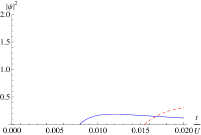
A plot of the condensate/superfluid density as a function of the tunneling parameter tt at a fixed value of the chemical potential μ\mu for each theory can be seen in Fig. 2.
Refer to caption
Refer to caption
Figure 2: Plot of the condensate density as a function of the hopping parameter t/U{t}/{U} for both the mean-field theory (left) and the effective action theory (right), with fixed μ/U=0.9{\mu}/{U}=0.9. The solid blue curves are T/U=0{T}/{U}=0, and the dashed red curves are T/U=0.1/kB{T}/{U}={0.1}/{k_{B}}.

It is interesting to note that while the superfluid density from the field-theoretic approach increases linearly with tt, the mean-field superfluid density quickly begins to fall off as tt increases, a behavior which is at odds with the notion of a superfluid [13]. Furthermore, it can be seen that Eq. (102) is simply a first order series expansion of Eq. (103) about t=tct=t_{c}, meaning |ψ|eq2\left|\psi\right|^{2}_{\mathrm{eq}} is the tangent line to |ψ|MF2\left|\psi\right|^{2}_{\mathrm{MF}} at t=tct=t_{c}. Thus, although the two results agree near the phase boundary, the mean-field prediction quickly begins to exhibit an unphysical behavior, suggesting that our field-theoretic result has a larger range of validity.

Refer to caption
Refer to caption
Figure 3: Plot of the average number of particles per site as a function of the chemical potential μ/U{\mu}/{U} with fixed t/U=0.025{t}/{U}=0.025. Left shows the mean-field prediction, while right shows the field-theoretic prediction. The solid blue curves are T/U=0{T}/{U}=0, and the dashed red curves are T/U=0.1/kB{T}/{U}={0.1}/{k_{B}}.
Refer to caption
Refer to caption
Figure 4: Plot of the compressibility κ​U{\kappa}{U} as a function of the chemical potential μ/U{\mu}/{U} with fixed t/U=0.025{t}/{U}=0.025. Left shows the mean-field prediction, while right shows the field-theoretic prediction. The solid blue curves are T/U=0{T}/{U}=0, and the dashed red curves are T/U=0.1/kB{T}/{U}={0.1}/{k_{B}}.

Next, we compare the average number of particles per lattice site ⟨n⟩\left<n\right> as computed in the two theories. In the ordered phase, the field theoretic prediction for ⟨n⟩\left<n\right> is given by Eq. (64) above, while the mean-field result is given by

⟨n⟩MF=−1Ns​∂ℱMF∂μ||ψ|2=|ψ|MF2.\left<n\right>_{\mathrm{MF}}=-\left.\frac{1}{N_{s}}\frac{\partial\mathcal{F}_{\mathrm{MF}}}{\partial\mu}\right|_{\left|\psi\right|^{2}=\left|\psi\right|^{2}_{\mathrm{MF}}}. (106)

In the Mott phase, |ψ|eq2=|ψ|MF2=0\left|\psi\right|^{2}_{\mathrm{eq}}=\left|\psi\right|^{2}_{\mathrm{MF}}=0, and both theories predict

⟨n⟩=⟨n⟩MF=−1N​∂F0∂μ,\left<n\right>=\left<n\right>_{\mathrm{MF}}=-\frac{1}{N}\frac{\partial F_{0}}{\partial\mu}, (107)

which is simply ⟨n⟩0\left<n\right>_{0}. Plots of these two quantities as a function of the chemical potential at a fixed value of the hopping parameter are shown in Fig. 3. Although the predictions of both theories agree in the immediate vicinity of the phase boundary, we see that at low temperatures ⟨n⟩MF\left<n\right>_{\mathrm{MF}} is not a monotonically increasing function of μ\mu. In fact, the plot shows that away from the phase boundary, ⟨n⟩MF\left<n\right>_{\mathrm{MF}} actually decreases with increasing μ\mu, i.e. the compressibility is predicted to be negative in the superfluid phase. This is directly at odds with the fact that a superfluid has, by definition, a positive compressibility [37]. The behavior of ⟨n⟩\left<n\right> as derived from the effective action, on the other hand, fits well with expectation further away from the phase boundary. This is highlighted in Fig. 4, which shows the compressibility κ\kappa for each case.

As a final point of comparison, we specify to the zero temperature case and examine contours in parameter space along which the average number density ⟨n⟩\left<n\right> is constant. Inside each Mott lobe, we know that the number density is fixed at the quantum number nn of the lobe. In the superfluid phase, for fixed tt we expect ⟨n⟩\left<n\right> to increase monotonically with increasing chemical potential. This implies that contours of constant ⟨n⟩\left<n\right> should be monotonic in μ\mu. Such contours for ⟨n⟩=1,2,3\left<n\right>=1,2,3 are shown in Fig. 5. Although the mean-field and effective action contours agree close to the lobe tip, the mean-field result exhibits a non-monotonic behavior farther away from the lobe tip. Given the non-monotonic behavior of ⟨n⟩MF\left<n\right>_{\mathrm{MF}} discussed above, this is not wholly surprising. From these considerations, we conclude that the effective action theory has a larger range of validity than the mean field theory and, furthermore, we expect an increase in quantitative accuracy when higher powers of tt are considered.

Refer to caption
Figure 5: Contours of constant ⟨n⟩\left<n\right> in parameter space for both the mean-field and effective action theories at T=0T=0. The dotted blue curve shows the first three lobes of the phase boundary. The solid blue curves are the predictions of the effective action theory, while the dotted red curves show the predictions of the mean-field theory.

VI.2 Effective Action Predictions in the Dynamic Case

We now turn our attention to the Green’s function and the zero-temperature excitation spectra of the Bose-Hubbard model. Using Eq. (77), we see that to first order in tt the Green’s function of the system in the ordered phase can be written as

𝒢⁡(ωm,k→)=a2(0)​(ωm)1+2a4(0)(ωm,0|0,ωm)(a2(0)(0))2[6t−1a2(0)​(0)](a2(0)(ωm))a4(0)(0,0|0,0)−2​t​a2(0)​(ωm)​∑σcos⁡(kσ​d),\mathcal{G}(\omega_{m},\vec{k})=\frac{a_{2}^{(0)}(\omega_{m})}{1+\frac{2a_{4}^{(0)}(\omega_{m},0|0,\omega_{m})(a_{2}^{(0)}(0))^{2}\left[6t-\frac{1}{a_{2}^{(0)}(0)}\right]}{(a_{2}^{(0)}(\omega_{m}))a_{4}^{(0)}(0,0|0,0)}-2ta_{2}^{(0)}(\omega_{m})\sum_{\sigma}\cos(k_{\sigma}d)}, (108)

where dd is the lattice spacing, and k→\vec{k} is restricted to the first Brillouin zone. At the phase boundary we have 6​t−1/a2(0)​(0)=06t-{1}/{a_{2}^{(0)}}(0)=0, and the Green’s function reduces to

𝒢⁡(ωm,k→)=a2(0)​(ωm)1−2​t​a2(0)​(ωm)​∑σcos⁡(kσ​d).\mathcal{G}(\omega_{m},\vec{k})=\frac{a_{2}^{(0)}(\omega_{m})}{1-2ta_{2}^{(0)}(\omega_{m})\sum_{\sigma}\cos(k_{\sigma}d)}. (109)

This is precisely the result obtained in the Mott phase via a resummation of zero loop diagrams [32].

From Eq. (84), we see that the zero-temperature dispersion relation for amplitude excitations ωA​(k→)\omega_{A}(\vec{k}) satisfies

0=−ia2​R(0)​(ωA)+2a4​R(0)(ωA,0|0,ωA)(a2​R(0)(0))2[6t+ia2​R(0)​(0)](a2​R(0)(ωA))2a4​R(0)(0,0|0,0)−2​t​∑σcos⁡(kσ​d),0=\frac{-i}{a_{2\mathrm{R}}^{(0)}(\omega_{\mathrm{A}})}+\frac{2a_{4\mathrm{R}}^{(0)}(\omega_{\mathrm{A}},0|0,\omega_{\mathrm{A}})(a_{2\mathrm{R}}^{(0)}(0))^{2}\left[6t+\frac{i}{a_{2\mathrm{R}}^{(0)}(0)}\right]}{(a_{2\mathrm{R}}^{(0)}(\omega_{\mathrm{A}}))^{2}a_{4\mathrm{R}}^{(0)}(0,0|0,0)}-2t\sum_{\sigma}\cos\left(k_{\sigma}d\right), (110)

which we recognize also as the condition for poles in Eq. (108) continued to real time. While too complicated to solve exactly, Eq. (110) can be inverted numerically to yield the dispersion relation ωA​(k→)\omega_{\mathrm{A}}(\vec{k}). A plot of ωA​(k→)\omega_{\mathrm{A}}(\vec{k}) taken along the (1,1,1)(1,1,1) direction in the first Brillouin zone is shown in Fig. 6. We observe that in the superfluid phase, ωA​(k→)\omega_{A}(\vec{k}) is gapped and quadratic,

ωA​(k→)≈Δ+η​k2.\omega_{A}(\vec{k})\approx\Delta+\eta k^{2}. (111)

Furthermore, at the phase boundary, we find that the dispersion becomes gapless and linear.

Next, we consider the zero-temperature dispersion relation ωθ​(k→)\omega_{\theta}(\vec{k}) of phase excitations. For the Bose-Hubbard model, Eq. (87) takes the form

0=\displaystyle 0= −ia2​R(0)​(ωθ)+ia2​R(0)​(0)−2​a2​R(0)​(0)3​(i+6​t​a2​R(0)​(0))a4​R(0)(0,0|0,0)[2b(0,0,0,0)+b(ωθ,−ωθ,0,0)\displaystyle\frac{-i}{a_{2\mathrm{R}}^{(0)}(\omega_{\theta})}+\frac{i}{a_{2\mathrm{R}}^{(0)}(0)}-\frac{2a_{2\mathrm{R}}^{(0)}(0)^{3}\left(i+6ta_{2R}^{(0)}(0)\right)}{a_{4\mathrm{R}}^{(0)}(0,0|0,0)}\Big[2b(0,0,0,0)+b(\omega_{\theta},-\omega_{\theta},0,0)\Big.
+b(0,0,ωθ,−ωθ)−2b(ωθ,0,ωθ,0)−2b(ωθ,0,0,ωθ)]+2t[3−∑σcos(kσd)].\displaystyle\Big.+b(0,0,\omega_{\theta},-\omega_{\theta})-2b(\omega_{\theta},0,\omega_{\theta},0)-2b(\omega_{\theta},0,0,\omega_{\theta})\Big]+2t\left[3-\sum_{\sigma}\cos\left(k_{\sigma}d\right)\right]. (112)

We can numerically solve this equation for ωθ​(k→)\omega_{\theta}(\vec{k}). A plot of ωθ​(k→)\omega_{\theta}(\vec{k}) along the (1,1,1)(1,1,1) direction in the first Brillouin zone is shown in the right of Fig. 6. We see that in the superfluid phase the dispersion is quadratic with

ωθ​(k→)≈ζ​k2.\omega_{\theta}(\vec{k})\approx\zeta k^{2}. (113)

Finally, by comparing Eqs. (110) and (112), we find that at the phase boundary ωA\omega_{A} and ωθ\omega_{\theta} are degenerate.

Refer to caption
Refer to caption
Figure 6: Plots of the zero-temperature dispersion relations ωA​(k→)\omega_{A}(\vec{k}) (Left) and ωθ​(k→)\omega_{\theta}(\vec{k}) (Right) for various values of the hopping tt with fixed n=1n=1, μ/U=2−1{\mu}/{U}=\sqrt{2}-1 and with k→=(1,1,1)​k/3\vec{k}=(1,1,1)k/\sqrt{3}. The solid blue lines corresponds to t=tc≈0.028​Ut=t_{c}\approx 0.028\,U, which for these values of μ\mu and nn is at the tip of the first Mott lobe. The dotted yellow lines corresponds to t=0.03​Ut=0.03\,U, and the dashed red lines corresponds to t=0.035​Ut=0.035\,U. Note that amplitude excitations exhibit a tt-dependent energy gap, while the phase excitations are gapless in accordance with Goldstone’s theorem.
Refer to caption
Figure 7: Plot of the second sound velocity cc as a function of t/Ut/U for t>tc≈0.028​Ut>t_{c}\approx 0.028\,U with nn=1 and μ/U=2−1{\mu}/{U}=\sqrt{2}-1.

Lastly, using the result (89), we can investigate the behavior of superfluid second sound excitations. From our observations above, we find a linear dispersion for small kk,

ωs​(k→)≈c​k\omega_{s}(\vec{k})\approx ck (114)

with the velocity of sound

c=Δ​ζ.c=\sqrt{\Delta\zeta}. (115)

Thus, the velocity of second sound at any point near the phase boundary can be found from the above numerical inversions. With this, we plot the sound velocity cc as a function of the tunneling t/Ut/U in Fig. 7. We observe that, since near the phase boundary a large quadratic term suddenly appears in the phase dispersion relation, the sound velocity jumps immediately inside the superfluid phase. This jump must be viewed cautiously, however, as the Ginzburg-Landau expansion is incapable of accurately describing critical behavior in the immediate vicinity of the phase boundary [27, 28, 41, 42]. As the mass of the phase excitations begins to increase faster than the gap in the amplitude excitations, we see that the sound velocity begins to decrease. Far from the phase boundary, however, we know from the seminal Bogoliubov theory that the sound velocity must increase as t\sqrt{t} [36, 43], confirming that our theory is not valid in the deep superfluid phase.

VII Summary and Conclusion

In this paper we derived, to first order in the tunneling, the Ginzburg-Landau expansion of the effective action for a very general Bosonic lattice Hamiltonian. From the effective action we calculated many static and dynamic system properties of experimental interest. In specifying these results to the Bose-Hubbard model, we compared them with the corresponding findings of the standard mean-field theory. Although both approaches yield – up to first order in the tunneling – the same phase boundary, our method gives qualitatively better results deeper in the superfluid phase. Additionally, we were able to find the dispersion relation for superfluid excitations, which cannot readily be done in the mean-field approach. The primary advantage of our effective-action theory, however, lies in its extensibility. It is straightforward to generalize the derivation given in Sections II and III by calculating diagrams beyond the tree level in order to include higher-order tunneling corrections. As seen in Section V, this gives a systematic hopping expansion of the self-energy function in both the ordered and non-ordered phases, providing an arbitrarily precise description of the system dynamics near the phase boundary. This should allow, for instance, for the calculation of time-of-flight absorption pictures and their corresponding visibilities for the whole phase diagram [35]. Furthermore, given the generality of the formalism, our effective action theory can, in principle, incorporate a variety of interesting effects, such as disordered lattices [4, 26], vortex dynamics [36], and tunneling beyond nearest neighbor sites. In particular, an effective action for the disordered Bose-Hubbard model could give new insight into the nature of the Bose glass phase as a state of short-range order [13].

Acknowledgements.
The authors thank Hagen Kleinert, Flavio Nogueira, and Matthias Ohliger for fruitful discussions and suggestions. Furthermore, we acknowledge financial support from both the German Academic Exchange Service (DAAD) and the German Research Foundation (DFG) within the Collaborative Research Center SBF/TR 12 Symmetries and Universality in Mesoscopic Systems.

References

  • [1] A. J. Legget, Rev. Mod. Phys. 73, 307 (2001).
  • [2] C. J. Pethick and H. Smith, Bose-Einstein Condensation in Dilute Gases (Cambridge University Press, Cambridge, 2002).
  • [3] L. Pitaevskii and S. Stringari, Bose-Einstein Condensation (Oxford Science Publications, Oxford, 2003).
  • [4] M. Lewenstein, A. Sanpera, V. Ahufinger, B. Damski, A. Sen(De), and U. Sen, Adv. Phys. 56, 243 (2007).
  • [5] I. Bloch, J. Dalibard, and W. Zwerger, Rev. Mod. Phys. 80, 885 (2008).
  • [6] M. Greiner, O. Mandel, T. Esslinger, T. W. Hänsch, and I. Bloch, Nature 415, 39 (2002).
  • [7] M. Greiner, O. Mandel, T.W. Hänsch, and I. Bloch, Nature, 419, 51 (2002).
  • [8] F. Gerbier, A. Widera, S. Fölling, O. Mandel, T. Gericke, and I Bloch, Phys. Rev. A 72, 053606 (2005).
  • [9] F. Gerbier, A. Widera, S. Fölling, O. Mandel, T. Gericke, and I Bloch, Phys. Rev. Lett. 95, 050404 (2005).
  • [10] S. Fölling, A. Widera, T. Müller, F. Gerbier, and I. Bloch, Phys. Rev. Lett. 97, 060403 (2006).
  • [11] K. Günter, T. Stöferle, H. Moritz, M Köhl, and T. Esslinger, Phys. Rev. Lett. 96, 180402 (2006).
  • [12] S. Ospelkaus, C. Ospelkaus, O. Wille, M. Succo, P. Ernst, K. Sengstock, and K. Bongs, Phys. Rev. Lett. 96, 180403 (2006).
  • [13] M. P. A. Fisher, P. B. Weichman, G. Grinstein, and D. S. Fisher, Phys. Rev. B 40, 546 (1989).
  • [14] D. Jaksch, C. Bruder, J. I. Cirac, C. W. Gardiner, and P. Zoller, Phys. Rev. Lett. 81, 3108 (1998).
  • [15] S. Sachdev, Quantum Phase Transitions (Cambridge University Press, Cambridge, 1999).
  • [16] D. Jaksch and P. Zoller, Ann. Phys. (New York) 315, 52 (2005).
  • [17] G. G. Batrouni, R. T. Scalettar, and G. T. Zimanyi, Phys. Rev. Lett. 65, 1765 (1990).
  • [18] B. Capogrosso-Sansone, S. G. Söyler, N. V. Prokof’ev, and B. V. Svistunov, Phys. Rev. A 77, 015602 (2008).
  • [19] B. Capogrosso-Sansone, E. Kozik, N. V. Prokof’ev, and B. V. Svistunov, Phys. Rev. A 75, 013619 (2007).
  • [20] J. K. Freericks and H. Monien, Phys. Rev. B 53, 2691 (1996).
  • [21] N. Elstner and H. Monien, Phys. Rev. B 59, 12184 (1999).
  • [22] F. E. A. dos Santos and A. Pelster, Phys. Rev. A 79, 013614 (2009).
  • [23] K. Ziegler, Physica A 208, 177 (1994).
  • [24] K. Ziegler, J. Low Temp. Phys. 126, 1431 (2002).
  • [25] K. Ziegler, Las. Phys. 13, 587 (2003).
  • [26] K. V. Krutitsky, A. Pelster, and R. Graham, New J. Phys. 8, 187 (2006).
  • [27] H. Kleinert and V. Schulte-Frohlinde, Critical Properties of ϕ4\phi^{4}-Theories (World Scientific, Singapore, 2001).
  • [28] J. Zinn-Justin, Quantum Field Theory and Critical Phenomena (Oxford University Press, New York, 2002).
  • [29] M. Peskin and D. Schröder, An Introduction to Quantum Field Theory (Westview Press, Boulder, 1995).
  • [30] M. P. Gelfand, R. R. P. Singh, and D. A. Huse, J. Stat. Phys. 59, 1093 (1990).
  • [31] W. Metzner, Phys. Rev. B 43, 8549 (1991).
  • [32] M. Ohliger, Dynamics and thermodynamics of spinor bosons in optical lattices, Diploma Thesis, Free University of Berlin (2008),
    http://users.physik.fu-berlin.de/˜ohliger/Diplom.pdf.
  • [33] M. E. Fischer, M. N. Barber, and D. Jasnow, Phys. Rev. A 8, 1111 (1973).
  • [34] R. Roth and K. Burnett, Phys. Rev. A 67, 031602(R) (2003).
  • [35] A. Hoffmann and A. Pelster, eprint: arXiv:0809.0771.
  • [36] H. Kleinert, Multivalued Fields: In Condensed Matter, Electromagnetism, and Gravitation (World Scientific, Singapore, 2008).
  • [37] P. B. Weichman, Phys. Rev. B 38, 8739 (1988).
  • [38] J. B. Bru and T. C. Dorlas, J. Stat. Phys. 113, 177 (2003).
  • [39] P. Buonsante and A. Vezzani, Phys. Rev. A 70, 033608 (2004).
  • [40] K. V. Krutitsky, M. Thorwart, R. Egger, and R. Graham, Phys. Rev. A 77, 053609 (2008).
  • [41] V. I. Ginzburg, Sov. Phys. Solid State 2, 1824 (1961).
  • [42] H. Kleinert, Phys. Rev. Lett. 84, 286 (2000).
  • [43] D. van Oosten, P. van der Straten, and H. T. C. Stoof, Phys. Rev. A 63, 053601 (2001).