Dynamics and transport of the $Z_{2}$ spin liquid:
application to $\kappa$-(ET)₂Cu₂(CN)₃

The dynamic spin correlations of $\mathcal{S}$ near the quantum critical point can be computed by the $1/N$ expansion on the O($N$) model, which has been described elsewhere [33]. With an eye towards possible future neutron scattering measurements, we first describe the dynamic spin susceptibility, $\chi(k,\omega)$ as a function of momentum $k$ and real frequency $\omega$. Here the momentum $k$ is measured as a deviation from the ordering wavevector, $Q$, of the antiferromagnetically ordered state. At $g=g_{c}$ and $T=0$, this has the quantum-critical form

where the exponent $\bar{\eta}$ is related to the scaling dimension of the composite spin operator $\sim z_{\alpha}\sigma^{y}_{\alpha\gamma}\vec{\sigma}_{\gamma\beta}z_{\beta}$ ($\vec{\sigma}$ are the Pauli matrices), and is known with high precision from field-theoretic studies [29] ($\bar{\eta}=1.374(12)$) and Monte Carlo simulations [30] ($\bar{\eta}=1.373(2)$). The overall amplitude $\mathcal{A}$ is non-universal, but the same $\mathcal{A}$ will appear in a number of results below. Integrating Eq. (2) over all $k$, we obtain the local susceptibility $\chi_{L}(\omega)$, which is also often measured in scattering experiments, again at $g=g_{c}$ and $T=0$

Let us now move into the spin liquid state, with $g>g_{c}$, where the spinons have an energy gap $\Delta_{z}$. The critical results in Eqs. (2) and (3) will apply for $|\omega|\gg\Delta_{z}$, but for $|\omega|\sim 2\Delta_{z}$, we will have spectra characteristic of the creation of a pair of spinons (we set $\hbar=1$, although it appears explicitly in a few expressions below). Computing the pair creation amplitude of non-interacting spinons, we obtain a step-discontinuity threshold at $\omega=\sqrt{c^{2}k^{2}+4\Delta_{z}^{2}}$ (at $T=0$). However, the spinons do have a repulsive interaction with each other, and this reduces the phase space for spinon creation at low momentum, as described in the supplementary material; the actual threshold behavior is:

where $\mathcal{C}$ is a universal constant; to leading order in the $1/N$ expansion, $\mathcal{C}=N^{2}/16$. We can also integrate the $k$-dependent generalization of Eq. (4) to obtain a threshold behavior for the local susceptibility at $2\Delta_{z}$: $\mbox{Im}\,\chi_{L}(\omega)\sim\mbox{sgn}(\omega)(|\omega|-2\Delta_{z})/\ln^{2}(|\omega|-2\Delta_{z})$.

Turning to the NMR relaxation rate, we have to consider $T>0$, and compute

This is far more subtle than the computations at $T=0$, because we have to compute the damping of the quantum critical excitations at $T>0$ and extend to the regime $\omega\ll T$. From general scaling arguments [33], we have

where $\Phi$ is a universal function. The computation of $\Phi$ for undamped spinons at $N=\infty$ is straightforward, and unlike the case for confining antiferromagnets [33], yields a reasonable non-zero answer: $\Phi(y)=[4\pi e^{y/2}(1+\sqrt{4+e^{y}})]^{-1}$. However, the $1/N$ corrections are singular, because $\Gamma$ has a singular dependence upon the spinon lifetime. A self-consistent treatment of the spinon damping is described in the supplementary material, and leads to the quantum-critical result ($\Delta_{z}=0$):

We now turn to the thermal transport co-efficient measured in the recent revealing experiments of Ref. 5. We consider the contribution of the spinons and visons in turn below, presenting further arguments on why the vison contribution can dominate in the experiments.

For agreement with the NMR measurements of $1/T_{1}$ [3], we need the spinons to be in the quantum critical regime, as described above. Therefore, we limit our considerations here to the quantum critical thermal conductivity of the spinons, $\kappa_{z}$, with $\Delta_{z}=0$. This can be obtained from the recent general theory of quantum critical transport [34] which yields

where $s$ is the entropy density of the spinons, and $1/\tau_{z}^{\rm imp}$ is the spinon momentum relaxation rate, with the $T$ dependence

Here $\nu$ is the critical exponent of the O(4) model [35], $\nu=0.749(2)$, and so $\tau_{z}^{\rm imp}\sim T^{-0.33}$. The two dimensional entropy density can be obtained from the results of Ref. 33:

where $\zeta$ is the Reimann zeta function. We estimate the co-efficient in Eq. (9) in the supplementary material using a soft-spin theory with the spinons moving in a random potential, $V(r)|z_{\alpha}|^{2}$, due to impurities of density $n_{\rm imp}$ each exerting a Yukawa potential $V_{q}=V_{z}/(q^{2}+\mu^{2})$; this leads to

Here $a$ is the spacing between the layers, and $T_{z}$ is the spinon bandwidth in temperature units and is proportional to the spinon velocity $c$.

The visons are thermally excited across an energy gap, $\Delta_{v}$, and so can be considered to be a dilute Boltzmann gas of particles of mass $m_{v}$. We assume there are $N_{v}$ species of visons. The visons see the background filling of spins as a magnetic flux through the plaquette on the dual lattice, and hence the dynamics of visons can be well described by a fully-frustrated quantum Ising model on the honeycomb lattice. Detailed calculations show that there are four minima of the vison band with an emergent O(4) flavor symmetry at low energy  [18], therefore $N_{v}=4$. As with the spinons, the visons are assumed to scatter off impurities of density $n_{\rm imp}$ with, say, a Yukawa potential $V_{q}=V_{v}/(q^{2}+\mu^{2})$. We use the fact that at low $T$, and for a large vison mass $m_{v}$, the visons are slowly moving. So each impurity scattering event can be described by a $T$-matrix $=[m_{v}\ln(1/k)/\pi]^{-1}$ characteristic of low momentum scattering in two dimensions. Application of Fermi’s golden rule then yields a vison scattering rate $1/\tau_{v}^{\rm imp}=\pi^{2}n_{\rm imp}/(m_{v}\ln^{2}(1/k))$. This formula becomes applicable when $\ln(1/k)\times V_{v}/(\hbar^{2}\mu^{2}/2m_{v})\gg 1$ i.e. the impurity potential becomes nonperturbative. We can now insert this scattering rate into a standard Boltzmann equation computation of the thermal conductivity $\kappa_{v}=2k_{B}^{2}Tn_{v}\tau_{v}^{\rm imp}/m_{v}$, where $n_{v}$ is the thermally excited vison density and the typical momentum $k\sim(m_{v}k_{B}T)^{1/2}$, to obtain

Here $T_{v}$ is some ultraviolet cutoff temperature which can be taken as the vison bandwidth. Note that for a large density of states of vison excitations, i.e. a large $m_{v}$, the prefactor of the exponential can be large. Similar calculations will not lead to a logarithmic divergence for the critical spinon $z$ due to the positive anomalous dimension of $|z|^{2}$, and therefore the impurity scattering of spinons is perturbative for $V_{z}/(c\mu\hbar)^{2}<1$.

Using Eq. (12), we fit the thermal conductivity measured by M. Yamashita et al. in Ref. 5 by tuning parameters $T_{v}$ and $\Delta_{v}$. The best fit values are $T_{v}=8.15K$, and $\Delta_{v}\equiv\Delta_{\kappa}=0.238K$, as shown in Fig. 1.

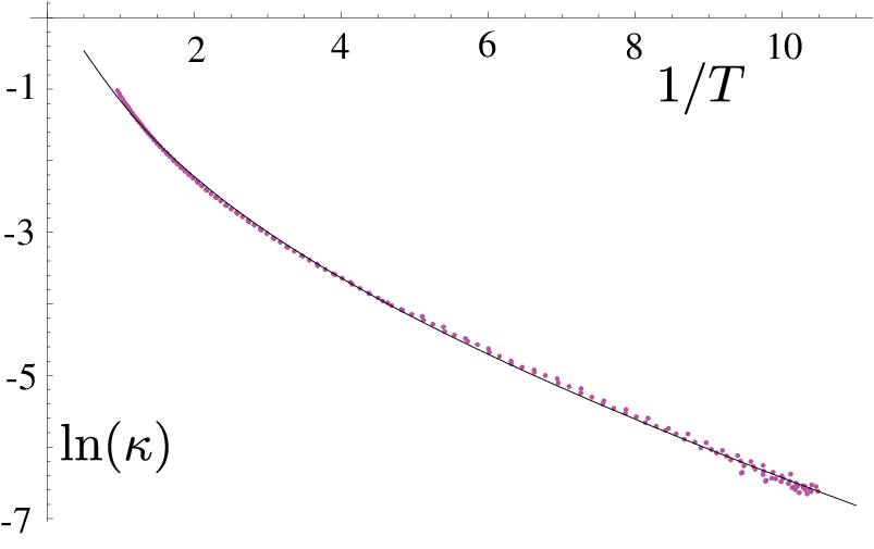
For consistency check, we calculate the ratio between the thermal conductivities contributed by spinons and visons using Eq. (11) and Eq. (12) and assuming moderate spinon impurity strength $V_{z}/(c\mu\hbar)^{2}\sim 1$:

We plot this ratio in Fig. 2, with $T_{z}\sim J_{2}=250$ K and other parameters as above, for the experimentally relevant temperature between $0.1$ K and $0.6$ K; we find consistency because $\kappa$ is dominated by the vison contribution. The vison dispersion is quadratic above the vison gap, and this leads to a $T$-independent $\gamma=C_{p}/T$ when $T>\Delta_{v}$, as observed in experiments [4]. Our estimate of the vison bandwidth, $T_{v}$, is also consistent with a peak in both $C_{P}$ [4] and $\kappa$ [5] at a temperature close to $T_{v}$.

The vison gap, $\Delta_{v}$, obtained here is roughly the same as the temperature at which the $1/T_{1}$ of NMR starts to deviate from the low temperature scaling of Eq. (6) [3]. When $T$ is above $\Delta_{v}$, thermally activated visons will proliferate. We discuss a theory of the spin dynamics in this thermal vison regime in the supplement, and find a $1/T_{1}$ with a weaker $T$ dependence compared to that present for $T<\Delta_{v}$. These observations are qualitatively consistent with the NMR data for 0.25 $<T<$ 10 K [3].

Ref. 5 also measured the thermal conductivity, in an applied field $H$ up to 10 T. There was little change in $\kappa$ for $H<4$ T. As $H$ couples to the conserved total spin, it only appears as an opposite “chemical potential” term for $z_{\alpha}$, modifying the temporal derivative $(\partial_{\tau}+(H/2)\sigma^{z})z^{\dagger}(\partial_{\tau}-(H/2)\sigma^{z})z$. At the quantum critical point, this term will induce a condensate of $z$ i.e. a non-collinear magnetically ordered state. We do not expect a significant difference in the thermal conductivity of the gapless spinons versus gapless spin-waves across this second order transition. We conjecture that the change at 4 T is associated with a vison condensation transition to a valence bond solid, as the field scale is or order the energy scales noted in the previous paragraph. This transition is possibly connected to the $H$-dependent broadening of the NMR spectra [3].

We have described the properties of a $Z_{2}$ spin liquid, on the verge of a transition to an magnetically ordered state, We have argued that the quantum critical spinons describe the NMR observations [3], while the visons (with a small energy gap and bandwidth) dominate the thermal transport [5].

We are very grateful to Minoru Yamashita for valuable discussions of the results of Ref. 5, and to the authors of Ref. 5 for permission to use their data in Fig. 1. We thank K. Kanoda, S. Kivelson, and T. Senthil for useful discussions. This research was supported by the NSF under grant DMR-0757145.

References

- [2] Y. Shimizu et al., Phys. Rev. Lett. 91, 107001 (2003).
- [3] Y. Shimizu et al., Phys. Rev. B 73, 140407(R) (2006).
- [4] S. Yamashita et al., Nature Physics 4, 459 (2008).
- [5] M. Yamashita et al., Nature Physics 5, 44 (2008).
- [6] O. I. Motrunich, Phys. Rev. B 72, 045105 (2005).
- [7] S.-S. Lee, P. A. Lee, and T. Senthil, Phys. Rev. Lett. 98, 067006 (2007).
- [8] Y. Qi and S. Sachdev, Phys. Rev. B 77, 165112 (2008).
- [9] P. Fazekas and P. W. Anderson, Philos. Mag. 30, 23 (1974).
- [10] S. A. Kivelson, D. S. Rokhsar, and J. P. Sethna, Phys. Rev. B 35, 8865 (1987).
- [11] B. J. Powell and R. H. McKenzie, J. Phys.: Condens. Matter 18, R827 (2006).
- [12] Y. Shimizu et al., J. Phys.: Condens. Matter 19, 145240 (2007).
- [13] N. Read and S. Sachdev, Phys. Rev. Lett. 66, 1773 (1991).
- [14] R. Jalabert and S. Sachdev, Phys. Rev. B 44, 686 (1991).
- [15] S. Sachdev, Phys. Rev. B 45, 12377 (1992).
- [16] N. Read and B. Chakraborty, Phys. Rev. B 40, 7133 (1989).
- [17] T. Senthil and M. P. A. Fisher, Phys. Rev. B 63, 134521 (2001).
- [18] R. Moessner and S. L. Sondhi, Phys. Rev. B 63, 224401 (2001).
- [19] A. Y. Kitaev, Annals of Physics 303, 2 (2003).
- [20] X. G. Wen, Phys. Rev. B 44, 2664 (1991); Phys. Rev. Lett. 90, 016803 (2003).
- [21] M. Freedman et al., Annals of Physics 310, 428 (2004).
- [22] F. Wang and A. Vishwanath, Phys. Rev. B 74, 174423 (2006).
- [23] G. Misguich and F. Mila, Phys. Rev. B 77, 134421 (2008).
- [24] W. LiMing et al., Phys. Rev. B 62, 6372 (2000).
- [25] R. R. P. Singh and D. A. Huse, Phys. Rev. Lett. 68, 1766 (1992).
- [26] M. Tamura, A. Nakao and R. Kato, J. Phys. Soc. Japan 75, 093701 (2006); Y. Shimizu et al., Phys. Rev. Lett. 99, 256403 (2007).
- [27] Z. Weihong, R. H. McKenzie, and R. R. P. Singh, Phys. Rev. B 59, 14367 (1999).
- [28] T. Itou, A. Oyamada, S. Maegawa, M. Tamura, and R. Kato, Phys. Rev. B 77, 104413 (2008).
- [29] P. Calabrese, A. Pelissetto, and E. Vicari, Phys. Rev. B 67, 054505 (2003).
- [30] S. V. Isakov, T. Senthil, and Y. B. Kim, Phys. Rev. B 72, 174417 (2005).
- [31] A. V. Chubukov, T. Senthil and S. Sachdev, Phys. Rev. Lett. 72, 2089 (1994).
- [32] P. Azaria, B. Delamotte, and T. Jolicoeur, Phys. Rev. Lett. 64, 3175 (1990).
- [33] A. V. Chubukov, S. Sachdev, and J. Ye, Phys. Rev. B 49, 11919 (1994).
- [34] S. A. Hartnoll et al., Phys. Rev. B 76, 144502 (2007); M. Müller and S. Sachdev, Phys. Rev. B 78, 115419 (2008)
- [35] M. Hasenbusch, J. Phys. A 34, 8221 (2001).
Dynamics and transport of the spin liquid:
application to -(ET)2Cu2(CN)3
Supplementary information.
Yang Qi, Cenke Xu, and Subir Sachdev
Department of Physics, Harvard University, Cambridge MA 02138, USA
(Dated: February 3, 2009)
This supplement presents additional details on computations in the main text. The large expansion of the nonlinear model field theory of the transition between the spin liquid and the phase with non-collinear magnetic order is presented in Section I. The thermal conductivity of the spinons is considered in Section II, and the NMR relaxation rate at temperatures above the vison gap is discussed in Section III.
I I. Large- expansion of nonlinear model
The phase transition between a non-collinear Néel state and spin liquid state can be described by the O(4) nonlinear model as in Eq. (1) in the main text
- [1] A. V. Chubukov, T. Senthil and S. Sachdev, Phys. Rev. Lett. 72, 2089 (1994).
- [2] C. Xu and S. Sachdev, Phys. Rev. B 79, 064405 (2009).
- [3] C. Timm, S. M. Girvin, P. Henelius and A. W. Sandvik, Phys. Rev. B 58, 1464 (1998).
- [4] A. V. Chubukov, S. Sachdev, and J. Ye, Phys. Rev. B 49, 11919 (1994).
- [5] Y. Shimizu et al., Phys. Rev. B 73, 140407(R) (2006).
- [6] S. A. Hartnoll et al., Phys. Rev. B 76, 144502 (2007); M. Müller and S. Sachdev, Phys. Rev. B 78, 115419 (2008).