Quasi-equilibrium models for triaxially deformed rotating compact stars

Xing Huang Affiliation: Department of Physics, University of Wisconsin-Milwaukee, P.O. Box 413, Milwaukee, WI 53201 Charalampos Markakis Affiliation: Department of Physics, University of Wisconsin-Milwaukee, P.O. Box 413, Milwaukee, WI 53201 Noriyuki Sugiyama Affiliation: Department of Physics, University of Wisconsin-Milwaukee, P.O. Box 413, Milwaukee, WI 53201 Kōji Uryū Affiliation: Department of Physics, University of the Ryukyus, Senbaru, Nishihara, Okinawa 903-0213, Japan

August 24, 2026

Abstract

Quasi-equilibrium models of rapidly rotating triaxially deformed stars are computed in general relativistic gravity, assuming a conformally flat spatial geometry (Isenberg-Wilson-Mathews formulation) and a polytropic equation of state. Highly deformed solutions are calculated on the initial slice covered by spherical coordinate grids, centered at the source, in all angular directions up to a large truncation radius. Constant rest mass sequences are calculated from nearly axisymmetric to maximally deformed triaxial configurations. Selected parameters are to model (proto-) neutron stars; the compactness is $M/R=0.001,0.1,0.14,0.2$ for polytropic index $n=0.3$ and $M/R=0.001,0.1,0.12,0.14$ for $n=0.5$ . We confirmed that the triaxial solutions exist for these parameters as in the case of Newtonian polytropes. However, it is also found that the triaxial sequences become shorter for higher compactness, and those may disappear at a certain large compactness for the $n=0.5$ case. In the scenario of the contraction of proto-neutron stars being subject to strong viscosity and rapid cooling, it is plausible that, once the viscosity driven secular instability sets in during the contraction, the proto-neutron stars are always maximally deformed triaxial configurations, as long as the compactness and the equation of state parameters allow such triaxial sequences. Detection of gravitational waves from such sources may be used as another probe for the nuclear equation of state.

I Introduction

Rapidly rotating compact objects are expected to be formed as new born neutron stars after stellar core collapses, or as differentially rotating hypermassive neutron stars after binary neutron star mergers. Accretion onto neutron stars in X-ray binaries can also lead to rapid rotation. All of these have been extensively studied as strong sources of gravitational waves for the ground based laser interferometers LIGO/GEO600/VIRGO/TAMA (See e.g. [1] and references therein).

Classical models of rotating stars are a class of ellipsoidal figures of equilibrium; self-gravitating rotating incompressible fluids in Newtonian gravity. Such solutions include sequences of axisymmetric Maclaurin ellipsoids, or non-axisymmetic Jacobi, Dedekind, or Riemann S-type ellipsoids [2]. These models are used to study the secular evolutions of rapidly rotating stars due to the viscosity and the radiation back-reaction of gravitational waves [3]. Lai and Shapiro [4] have developed an ellipsoidal approximation to the rotating polytropes, and applied the model to clarify the secular evolution of rapidly rotating neutron stars in detail, and more recently focused on the viscosity driven secular instability [5].

As discussed in [1, 3, 4], and shown by a number of numerical simulations of rapidly rotating compact stars, core collapse, and binary neutron star mergers [6, 7, 8], a transient triaxially deformed compact object may survive within a secular time scale. In this paper, we consider uniformly rotating models of such triaxially deformed compact objects, an extension of the Jacobi ellipsoid in general relativity. In Newtonian gravity, such solutions exist for rotating polytropes with polytropic index $n<0.808$ [9]. Here, the polytropic equation of state (EOS) $p=\kappa\rho^{1+1/n}$ relates the pressure $p$ with the baryon rest mass density $\rho$ .

In general relativity, such configurations are not in equilibrium due to the back-reaction of gravitational radiation. However as in the case of quasi-equilibrium initial data of binary neutron stars, triaxially deformed uniformly rotating stars are in quasi-equilibrium, as long as the gravitational luminosity is small enough that the energy radiated away within a rotational period is small compared to the binding energy of the star, which is always the case, and if the viscosity is strong enough for the flow field to become uniformly rotating during the evolution. Therefore, as an important application, a sequence of uniformly rotating quasi-equilibrium solutions may model a secular evolution from the proto-neutron star to the neutron star in the strong viscosity limit, and each solution may serve as the initial data for the general relativistic hydrodynamic simulations of such objects.

Models of rapidly rotating neutron stars have been extensively studied as stationary, axisymmetric, perfect-fluid spacetimes [10], while less attention has been paid to uniformly rotating triaxial solutions, not only because they are not exact equilibria due to gravitational radiation reaction, but also because, in early calculations [11], models of the EOS above nuclear density did not allow large enough values of $T/|W|\sim 0.14$ where a triaxial sequence is expected to bifurcate from an axisymmetric sequence. Here, $T/|W|$ is the ratio of kinetic energy $T$ to gravitational potential energy $W$ . However, as seen, for example, in [12], a value $n\sim 0.5$ (an effective adiabatic index $\Gamma\sim 3$ ) may be possible for recent models of EOS for high density nuclear matter, above $\rho>\rho_{\rm nuc}\sim 2\times 10^{14}{\rm g/cm}^{3}$ , and, as we will see below, triaxial quasi-equilibrium solutions do exist even in strong gravity for relatively small polytropic indexes, such as $n=0.5$ or $n=0.3$ , as in the Newtonian case.

About a decade ago, Nozawa succeeded in computing uniformly rotating triaxial polytropes in general relativistic gravity in his thesis [13], although his calculations were limited by the computational resources to low resolutions. A few studies approximating the fluid as an ellipsoidal configuration in general relativistic gravity have been made [14], and perturbative analyses have located the bifurcation point suggesting the existence of solutions having triaxial bar-mode deformations [15, 17, 18, 19, 20, 16]. Our computations of triaxially deformed stars can be used to locate the instability points on the axisymmetric sequence as well as to estimate the gravitational wave amplitude and luminosity from such objects.

In this paper, we present our first results on triaxial configurations of rapidly rotating general relativistic stars as models of neutron stars in extreme rotation. We assume a conformally flat spatial slice, and solve the constraints and spatial trace of the Einstein equation (Isenberg-Wilson-Mathews (IWM) formulation) [21, 22] ¹¹ 1 The validity of the IWM formulation for axisymmetric configurations is discussed in [23, 24]. This is different from the formulation used by Nozawa [13] in which the line element is chosen to be the same form as that of stationary axisymmetric spacetime, but an azimuthal dependence is allowed (see [25] for the same formulation). The formulations and the code are described in the next section. For testing the code, selected axisymmetric solutions are compared with the results in the literature, and the bifurcation points of axisymmetric and triaxial sequences in weak gravity are examined. Then, we present the results of deformation sequences of constant rest mass systematically in the range of two parameters, the compactness $M/R$ and the polytropic index $n$ , appropriate for realistic neutron stars. Applications of such triaxial solutions in the contraction of a newly born proto-neutron star are briefly discussed in the final section. Throughout the paper, we use units such that $G=c=1$ . For our tensor notation, we adopt the use of Greek letters for spacetime indices, and Latin letters for spatial indices.

II Formulation and numerical method

II.1 IWM formulation

The IWM formulation for computing spatially conformally flat initial data we use for computing non-axisymmetric quasi-equilibrium of rotating compact star is briefly described. The spacetime ${\cal M}={\mathbb{R}}\times\Sigma$ is foliated by the family of spacelike hypersurfaces $\Sigma_{t}=\{t\}\times\Sigma$ . The future-pointing timelike normal $n^{\alpha}$ to $\Sigma_{t}$ is related to the timelike vector $t^{\alpha}$ , which is tangent to a curve $t\rightarrow(t,x),\ x\in\Sigma$ , by $t^{\alpha}=\alpha n^{\alpha}+\beta^{\alpha}$ , where $\alpha$ is the lapse, and $\beta^{\alpha}$ the shift which satisfies $\beta^{\alpha}n_{\alpha}=0$ . Restricting the projection tensor $\gamma_{{\alpha\beta}}=g_{\alpha\beta}+n_{\alpha}n_{\beta}$ , a spatial metric $\gamma_{ab}(t)$ is defined on $\Sigma_{t}$ . In the IWM formulation, the spatial metric is chosen to be conformally flat, $\gamma_{ab}=\psi^{4}f_{ab}$ , where $f_{ab}$ is a flat metric on each slice, and $\psi$ is a conformal factor. Then the metric $g_{\alpha\beta}$ takes the form

ds^{2}=-\alpha^{2}dt^{2}+\psi^{4}f_{ij}(dx^{i}+\beta^{i}dt)(dx^{j}+\beta^{j}dt),

(1)

in a chart $\{t,x^{i}\}$ . The extrinsic curvature of the foliation is defined by

K_{ab}\,:=\,-\frac{1}{2\alpha}\partial_{t}\gamma_{ab}+\frac{1}{2\alpha}\mbox{\pounds}_{\beta}\gamma_{ab}.

(2)

In the IWM formulation, the Einstein equation is decomposed with respect to the foliation, and the following 5 components Eqs.(3)-(5) are chosen to be solved for the five metric coefficients $\{\psi,\alpha,\beta^{a}\}$ on the initial slice $\Sigma_{0}$ :

	$\displaystyle(G_{\alpha\beta}-8\pi T_{\alpha\beta})\,n^{\alpha}n^{\beta}\ \,=\,0,$		(3)
	$\displaystyle(G_{\alpha\beta}-8\pi T_{\alpha\beta})\,\gamma_{a}{}^{\alpha}n^{\beta}\,=\,0,$		(4)
	$\displaystyle(G_{\alpha\beta}-8\pi T_{\alpha\beta})\,\Big(\gamma^{{\alpha\beta}}+\frac{1}{2}n^{\alpha}n^{\beta}\Big)\,=\,0,$		(5)

where the first and second equations are the constraints. These equations are written in the form of elliptic equations with the non-linear source terms, respectively,

	$\displaystyle{\raise 4.30554pt\hbox{${}^{\ \circ}$}}\!\!\!\!\Delta\psi\,=\,-\frac{\psi^{5}}{8}\left(A_{ab}A^{ab}+\frac{2}{3}K^{2}\right)-2\pi\psi^{5}\rho_{\rm H},$		(6)
	$\displaystyle{\raise 4.30554pt\hbox{${}^{\ \circ}$}}\!\!\!\!\Delta\tilde{\beta}_{a}+\frac{1}{3}{\raise 4.30554pt\hbox{${}^{\ \circ}$}}\!\!\!\!\!D_{a}{\raise 4.30554pt\hbox{${}^{\ \circ}$}}\!\!\!\!\!D_{b}\tilde{\beta}^{b}\,=\,-2\alpha A_{a}{}^{b}{\raise 4.30554pt\hbox{${}^{\ \circ}$}}\!\!\!\!\!D_{b}\ln\frac{\psi^{6}}{\alpha}+\frac{4}{3}\alpha{\raise 4.30554pt\hbox{${}^{\ \circ}$}}\!\!\!\!\!D_{a}K$
	$\displaystyle\qquad\qquad\qquad+16\pi\alpha j_{a},$		(7)
	$\displaystyle{\raise 4.30554pt\hbox{${}^{\ \circ}$}}\!\!\!\!\Delta(\alpha\psi)\,=\,-\psi^{5}\left(\partial_{t}-\mbox{\pounds}_{\beta}\right)K$
	$\displaystyle\ +\alpha\psi^{5}\left(\frac{7}{8}A_{ab}A^{ab}+\frac{5}{12}K^{2}\right)+2\pi\alpha\psi^{5}(\rho_{\rm H}+2S),$		(8)

where $K$ is the trace of $K_{ab}$ , $A_{ab}$ its tracefree part, $\tilde{\beta}_{a}$ the conformally weighted shift defined by $\tilde{\beta}_{a}=f_{ab}\tilde{\beta}^{b}$ and $\tilde{\beta}^{a}=\beta^{a}$ , ${\raise 4.30554pt\hbox{${}^{\ \circ}$}}\!\!\!\!\Delta$ is the flat Laplacian and ${\raise 4.30554pt\hbox{${}^{\ \circ}$}}\!\!\!\!\!D_{a}$ is the covariant derivative with respect to the flat three-metric $f_{ab}$ . The source terms of matter are defined by $\rho_{\rm H}:=T_{\alpha\beta}n^{\alpha}n^{\beta}$ , $j_{a}:=-T_{\alpha\beta}\gamma_{a}{}^{\alpha}n^{\beta}$ , and $S:=T_{\alpha\beta}\gamma^{\alpha\beta}$ . Expressions of the sources in terms of the metric potentials and fluid variables are given in Appendix A.

We choose a maximally embedded slice $K=0=\partial_{t}K$ . Because the spatial metric is conformally flat, $A_{ab}$ does not involve time derivatives of the spatial metric,

	$\displaystyle A_{ab}$	$\displaystyle=$	$\displaystyle\frac{\psi^{4}}{2\alpha}\left(\mbox{\pounds}_{\beta}f_{ab}-\frac{1}{3}f_{ab}f^{cd}\mbox{\pounds}_{\beta}f_{cd}\right)$		(9)
		$\displaystyle=$	$\displaystyle\frac{\psi^{4}}{2\alpha}\left({\raise 4.30554pt\hbox{${}^{\ \circ}$}}\!\!\!\!\!D_{a}\tilde{\beta}_{b}+{\raise 4.30554pt\hbox{${}^{\ \circ}$}}\!\!\!\!\!D_{b}\tilde{\beta}_{a}-\frac{2}{3}f_{ab}{\raise 4.30554pt\hbox{${}^{\ \circ}$}}\!\!\!\!\!D_{c}\beta^{c}\right)$		(10)

where $\mbox{\pounds}_{\beta}$ denotes the Lie derivative with respect to $\beta^{a}$ . The field equations Eqs.(6)-(8) are thus rewritten

	$\displaystyle\!\!\!\!\!\!\!{\raise 4.30554pt\hbox{${}^{\ \circ}$}}\!\!\!\!\Delta\psi\,=\,-\frac{\psi^{5}}{8}A_{ab}A^{ab}-2\pi\psi^{5}\rho_{\rm H},$		(11)
	$\displaystyle\!\!\!\!\!\!\!{\raise 4.30554pt\hbox{${}^{\ \circ}$}}\!\!\!\!\Delta\tilde{\beta}_{a}+\frac{1}{3}{\raise 4.30554pt\hbox{${}^{\ \circ}$}}\!\!\!\!\!D_{a}{\raise 4.30554pt\hbox{${}^{\ \circ}$}}\!\!\!\!\!D_{b}\tilde{\beta}^{b}\,=\,-2\alpha A_{a}{}^{b}{\raise 4.30554pt\hbox{${}^{\ \circ}$}}\!\!\!\!\!D_{b}\ln\frac{\psi^{6}}{\alpha}+16\pi\alpha j_{a},$		(12)
	$\displaystyle\!\!\!\!\!\!\!{\raise 4.30554pt\hbox{${}^{\ \circ}$}}\!\!\!\!\Delta(\alpha\psi)\,=\,\frac{7}{8}\alpha\psi^{5}A_{ab}A^{ab}+2\pi\alpha\psi^{5}(\rho_{\rm H}+2S).$		(13)

Eq.(12) is decomposed further to improve the accuracy in numerical computation. Following the decomposition proposed by Shibata [26], we write Eq.(12) as

{\raise 4.30554pt\hbox{${}^{\ \circ}$}}\!\!\!\!\Delta\tilde{\beta}_{a}+\frac{1}{3}{\raise 4.30554pt\hbox{${}^{\ \circ}$}}\!\!\!\!\!D_{a}{\raise 4.30554pt\hbox{${}^{\ \circ}$}}\!\!\!\!\!D_{b}\tilde{\beta}^{b}={\cal S}_{a},

(14)

and introduce

\tilde{\beta}_{a}=B_{a}+\frac{1}{8}{\raise 4.30554pt\hbox{${}^{\ \circ}$}}\!\!\!\!\!D_{a}(B-x^{b}B_{b}),

(15)

where $x^{a}$ are coordinates that satisfy ${\raise 4.30554pt\hbox{${}^{\ \circ}$}}\!\!\!\!\!D_{a}x^{b}=\delta_{a}{}^{b}$ . Substituting the decomposition (15) into Eq.(14) yields

{\raise 4.30554pt\hbox{${}^{\ \circ}$}}\!\!\!\!\Delta\tilde{\beta}_{a}+\frac{1}{3}{\raise 4.30554pt\hbox{${}^{\ \circ}$}}\!\!\!\!\!D_{a}{\raise 4.30554pt\hbox{${}^{\ \circ}$}}\!\!\!\!\!D_{b}\tilde{\beta}^{b}\,=\,{{\raise 4.30554pt\hbox{${}^{\ \circ}$}}\!\!\!\!\Delta B_{a}}+\frac{1}{6}{\raise 4.30554pt\hbox{${}^{\ \circ}$}}\!\!\!\!\!D_{a}({{\raise 4.30554pt\hbox{${}^{\ \circ}$}}\!\!\!\!\Delta B-x^{b}{\raise 4.30554pt\hbox{${}^{\ \circ}$}}\!\!\!\!\Delta B_{b}})\,=\,{{\cal S}_{a}}.

(16)

The elliptic equations ${\raise 4.30554pt\hbox{${}^{\ \circ}$}}\!\!\!\!\Delta B_{a}={\cal S}_{a}$ and ${\raise 4.30554pt\hbox{${}^{\ \circ}$}}\!\!\!\!\Delta B-x^{b}{\raise 4.30554pt\hbox{${}^{\ \circ}$}}\!\!\!\!\Delta B_{b}=0$ are separated, and the former is substituted to the latter:

	$\displaystyle{\raise 4.30554pt\hbox{${}^{\ \circ}$}}\!\!\!\!\Delta B_{a}\,=\,{\cal S}_{a}\,:=\,-2\alpha A_{a}{}^{b}{\raise 4.30554pt\hbox{${}^{\ \circ}$}}\!\!\!\!\!D_{b}\ln\frac{\psi^{6}}{\alpha}+16\pi\alpha j_{a},$		(17)
	$\displaystyle{\raise 4.30554pt\hbox{${}^{\ \circ}$}}\!\!\!\!\Delta B\,=\,x^{a}{\cal S}_{a}.$		(18)

The potentials $\{B_{a},B\}$ are solved for simultaneously, and the shift $\tilde{\beta}_{a}$ is reconstructed from Eq.(15).

II.2 Formulation for a relativistic fluid in equilibrium

A perfect fluid is described by the stress-energy tensor

T_{\alpha\beta}=(\epsilon+p)u_{\alpha}u_{\beta}+pg_{\alpha\beta},\qquad

(19)

where $u^{\alpha}$ is the 4-velocity of the fluid, $p$ its pressure, and $\epsilon$ the energy density. As a consequence of the Bianchi identity, the stress-energy tensor is covariantly conserved:

\nabla_{\beta}T_{\alpha}{}^{\beta}=0.

(20)

When the fluid is close to equilibrium, one can obtain a simpler set of equations. Introducing the specific enthalpy defined by $h:=(\epsilon+p)/\rho$ , where $\rho$ is the baryon rest mass density, the left hand side of Eq. (20) can be written

	$\displaystyle{\nabla_{\beta}T_{\alpha}{}^{\beta}}$	$\displaystyle=$	$\displaystyle\rho\biggl[\,{u^{\beta}\nabla_{\beta}(hu_{\alpha})+\nabla_{\alpha}h}\,\biggr]$		(21)
			$\displaystyle\,+\,hu_{\alpha}{\nabla_{\beta}(\rho u^{\beta})}\,-\,\rho T{\nabla_{\alpha}s},$		(21)

where $s$ is the specific entropy. In the derivation, the local first law of thermodynamics $dh=Tds+dp/\rho$ was used. In local thermodynamic equilibrium, one can also assume the conservation of baryon mass,

\nabla_{\alpha}(\rho u^{\alpha})\,=\,\frac{1}{\sqrt{-g}}\mbox{\pounds}_{u}(\rho\sqrt{-g})\,=\,0.

(22)

Consequently, the conservation of specific entropy along the fluid world line,

u^{\alpha}\nabla_{\alpha}s=\mbox{\pounds}_{u}s=0,

(23)

and, the relativistic Euler equations,

u^{\beta}\nabla_{\beta}(hu_{\alpha})+\nabla_{\alpha}h\,=\,\mbox{\pounds}_{u}(hu_{\alpha})+\nabla_{\alpha}h\,=\,0,

(24)

are obtained. Assuming the flow field to be isentropic everywhere inside the neutron star matter, $s=\rm const$ , we have a one-parameter equations of state (EOS) $p=p(\rho)$ .

We assume a stationary state in the rotating frame for the fluid source. Imposing symmetry along the helical vector $k^{\alpha}=t^{\alpha}+\Omega\phi^{\alpha}$ where $\Omega$ is a constant angular velocity of a rotating frame, we have

\mbox{\pounds}_{k}(\rho u^{t}\sqrt{-g})=0,\ \ \mbox{and}\ \ \gamma_{a}\!^{\alpha}\mbox{\pounds}_{k}(hu_{\alpha})=0,

(25)

with $u^{t}$ interpreted as the scalar $u^{\alpha}\nabla_{\alpha}t$ . For a corotational flow, $u^{\alpha}=u^{t}k^{\alpha}$ , the rest mass conservation becomes trivial, and the relativistic Euler equation has the first integral

\frac{h}{u^{t}}\,=\,{\cal E}\,=\,\mbox{constant},

(26)

where ${\cal E}$ is the injection energy. From the normalization of the four velocity $u_{\alpha}u^{\alpha}=-1$ , one obtains

u^{t}=\frac{1}{\sqrt{\alpha^{2}-\omega_{a}\omega^{a}}}=\frac{1}{\sqrt{\alpha^{2}-\psi^{4}f_{ab}\,\omega^{a}\omega^{b}}},

(27)

where $\omega^{a}=\beta^{a}+\Omega\phi^{a}$ .

As a first step in the calculation of a highly deformed triaxial compact star, we assume a simple polytropic EOS,

p=\kappa\rho^{1+1/n},

(28)

where $\kappa$ is a constant, and $n$ is the polytropic index. Then $h$ is related to $p/\rho$ by

h=1+(n+1)\frac{p}{\rho}.

(29)

We also refer to the polytropic exponent $\Gamma$ defined by $\Gamma:=1+1/n$ .

II.3 Numerical computation

The Poisson solver and the iteration scheme used to solve the system of elliptic equations with non-linear source terms, are similar to the ones used in a previously developed initial data code for binary black holes and neutron stars [27, 28]. However, the code itself has been completely rewritten, so that further extensions can be incorporated easily. One of the revisions of the code is that no symmetry is a priori assumed on the spatial slice $\Sigma_{0}$ ; that is, the spherical coordinate grids centered at the source cover all angular directions, up to a certain large truncation radius. Hence, for example, asymmetric magnetic fields may be later included without major modifications to the code. Computation of binary solutions using the same coordinate setup is also possible. The other major change is a simpler, more robust choice of finite differencing. In this section, we briefly describe the necessary steps for constructing the code, which are 1. Spherical coordinates and the length scale, 2. Summary of variables and equations for coding, 3. Poisson solver, 4. Grid spacing, 5. Finite differencing and iteration, 6. Computation of a sequence of solutions.

II.3.1 Spherical coordinates and the length scale

The slice $\Sigma_{0}$ is covered by a spherical coordinate patch $(r,\theta,\phi)\in[r_{a},r_{b}]\times[0,\pi]\times[0,2\pi]$ . For a single star calculation, the radial coordinate extends from the center of the star $r=r_{a}=0$ to the asymptotic radius $r=r_{b}=10^{4}R_{0}$ , where $R_{0}$ is the radius of the neutron star along the semi-major axis, defined by the $\theta=\pi/2$ and $\phi=0,\pi$ lines. We also refer to Cartesian coordinates $(x,y,z)$ whose positive $x$ , $y$ and $z$ directions are along $(\theta,\phi)=(\pi/2,0)$ , $(\pi/2,\pi/2)$ and $\theta=0$ , respectively.

The quantity $R_{0}$ is introduced as an additional parameter in the formulation used in our code, normalizing the radial coordinate as

\hat{r}=r/R_{0}.

(30)

For a polytropic EOS, one can rescale the length using the polytropic constant $\kappa$ as $\kappa^{-n/2}R_{0}$ , or simply setting $\kappa=1$ (see e.g. [27]). As a result, we have three parameters $\{\Omega,{\cal E},R_{0}\}$ in our formulation.

Furthermore, we introduce surface fitted coordinates on which the fluid variables are defined. Assuming that the surface of a neutron star can be described by a function of the angular coordinate $R(\theta,\phi)=R_{0}\hat{R}(\theta,\phi)$ , the surface fitted coordinates $(\hat{r}_{\rm f},\theta_{\rm f},\phi_{\rm f})$ are defined by

\hat{r}_{\rm f}:=\hat{r}/\hat{R}(\theta,\phi),\ \ \theta_{\rm f}=\theta,\ \ \phi_{\rm f}=\phi,

(31)

where $\hat{r}_{\rm f}$ is defined in a region $\hat{r}_{\rm f}\in[0,1]$ .

II.3.2 Summary of variables and equations for coding

As mentioned in Sec. II.1, the field equations (11), (13), (17) and (18) are solved for the metric potentials $\{\psi,\alpha\psi,B^{a},B\}$ and, as in Sec. II.2 and II.3.1, a comoving fluid in equilibrium is characterized by one fluid variable, which is chosen to be the relativistic enthalpy $\{h\}$ , and three parameters $\{\Omega,{\cal E},R_{0}\}$ .

The field equations are normalized to have the following form; representing each of the metric potentials $\{\psi,\alpha\psi,B^{a},B\}$ by $\Phi$ ,

{\raise 4.30554pt\hbox{${}^{\ \circ}$}}\!\!\!\!\Delta\Phi\,=\,S_{\rm g}\,+\,R_{0}^{2}\,S_{\rm m},

(32)

where the flat Laplacian ${\raise 4.30554pt\hbox{${}^{\ \circ}$}}\!\!\!\!\Delta$ corresponds now to the normalized coordinate $\hat{r}$ . The source term $S_{\rm g}$ includes the metric potentials and their derivatives, while $S_{\rm m}$ also includes the matter variables and the parameters $\{\Omega,\cal E\}$ , while the dependence on the length scale $R_{0}$ is explicitly separated in Eq.(32).

The fluid variable $\{h\}$ is determined by Eq.(26) coupled to the EOS (28), and the relations (27) and (29). The three parameters $\{\Omega,{\cal E},R_{0}\}$ are determined by the following three quantities: the surface radii along two of the three semi-major axes, and the value of the central density. These quantities are used to impose three conditions on Eq.(26), which are solved with respect to the three parameters $\{\Omega,{\cal E},R_{0}\}$ in each iteration cycle.

II.3.3 Poisson solver

The elliptic equations (11), (13) (17), and (18) are integrated on the spherical grid using Green’s formula. Representing each of the potentials $\{\psi,\alpha\psi,B^{a},B\}$ by $\Phi$ , the latter is given by

$\displaystyle\Phi(x)$	$\displaystyle=$	$\displaystyle-\frac{1}{4\pi}\int_{V}G(x,x^{\prime})S(x^{\prime})d^{3}x^{\prime}$	(33)
		$\displaystyle+\frac{1}{4\pi}\int_{\partial V}\left[G(x,x^{\prime})\nabla^{\prime a}\Phi(x^{\prime})\right.$
		$\displaystyle\qquad\qquad\left.-\Phi(x^{\prime})\nabla^{\prime a}G(x,x^{\prime})\right]dS^{\prime}_{a}.$

where $x$ and $x^{\prime}$ are positions, $x,x^{\prime}\in V\subseteq\Sigma_{0}$ . We choose the Green function $G(x,x^{\prime})$ without boundary,

{\raise 4.30554pt\hbox{${}^{\ \circ}$}}\!\!\!\!\Delta G(x,x^{\prime})=-4\pi\delta(x-x^{\prime}),

(34)

and perform a multipole expansion in associated Legendre functions,

	$\displaystyle G(x,x^{\prime})=\frac{1}{\left\|{x}-{x^{\prime}}\right\|}\,=\,\sum_{\ell=0}^{\infty}g_{\ell}(r,r^{\prime})\sum_{m=0}^{\ell}\epsilon_{m}\,\frac{(\ell-m)!}{(\ell+m)!}$
	$\displaystyle\qquad\quad\times P_{\ell}^{~m}(\cos\theta)\,P_{\ell}^{~m}(\cos\theta^{\prime})\cos m(\varphi-\varphi^{\prime}),$		(35)

where the radial Green function $g_{\ell}(r,r^{\prime})$ is defined by

g_{\ell}(r,r^{\prime})=\frac{r_{<}^{\ell}}{r_{>}^{\ell+1}},\quad r_{>}:=\sup\{r,r^{\prime}\},\ r_{<}:=\inf\{r,r^{\prime}\},

(36)

and the coefficients $\epsilon_{m}$ are equal to $\epsilon_{0}=1$ for $m=0$ , and $\epsilon_{m}=2$ for $m\geq 1$ .

II.3.4 Grid spacing

The field equations in the integral form (33) are discretized on the spherical grids, and iterated until convergence is achieved. Our code allows us to use any non-equidistant grid spacing in all the spatial coordinates, $(r_{i},\theta_{j},\phi_{k})$ , $i=0,\cdots,N_{r}$ , $j=0,\cdots,N_{\theta}$ , and $k=0,\cdots,N_{\phi}$ . The radial grid points are equidistant in the region $[r_{a},r_{c}]$ and non-equidistant in $[r_{c},r_{b}],$ as follows: writing $\Delta r_{i}:=r_{i}-r_{i-1}$ , we have

	$\displaystyle\Delta r_{i}=\Delta r=\frac{r_{c}-r_{a}}{n_{r}}\quad\mbox{for}\quad i=1,\cdots,n_{r},$		(37)
	$\displaystyle\Delta r_{i}=k\Delta r_{i-1}\qquad\mbox{for}\quad i=n_{r}+1,\cdots,N_{r},$		(38)

where the constant $k$ is determined from the relation

r_{b}-r_{c}=\frac{k^{N_{r}-n_{r}+1}-k}{k-1}\Delta r\>.

(39)

We choose equidistant grid spacing for $\theta_{j}$ and $\phi_{k}$ , that is, $\Delta\theta_{i}=\Delta\theta=\pi/N_{\theta}$ , and $\Delta\phi_{i}=\Delta\phi=2\pi/N_{\phi}$ . Our notations for the grid points are summarized in Table 1.

$r_{a}$	:	Radial coordinate where the grid $r_{i}$ starts.
$r_{b}$	:	Radial coordinate where the grid $r_{i}$ ends.
$r_{c}$	:	Radial coordinate between $r_{a}$ and $r_{b}$ where the
		grid changes from equidistant to non-equidistant.
$N_{r}$	:	Total number of intervals $\Delta r_{i}$ between $r_{a}$ and $r_{b}$ .
$n_{r}$	:	Number of intervals $\Delta r_{i}$ between $r_{a}$ and $r_{c}$ .
$N_{\hat{r}}$	:	Total number of intervals $\Delta\hat{r}_{i}$ for $\hat{r}\in[\hat{r}_{a},\hat{R}(\theta,\phi)]$ .
$N_{\theta}$	:	Total number of intervals $\Delta\theta_{i}$ for $\theta\in[0,\pi]$ .
$N_{\phi}$	:	Total number of intervals $\Delta\phi_{i}$ for $\phi\in[0,2\pi]$ .

Table 1: Summary of grid parameters.

II.3.5 Finite differencing and iteration

For the numerical integration of Eq.(33) we select the mid-point rule. Accordingly, source terms are evaluated at the middle of successive grid points. The linear interpolation formula and the second order Lagrange formula are applied for computing the source term fields and their derivatives respectively, at the mid-points of the $r$ , $\theta$ and $\phi$ grids.

The reason for selecting a rather low (second) order finite difference scheme is the following: When the field quantities vary rapidly, such as at a density discontinuity in a neutron star, higher order interpolating formulas as well as finite difference formulas tend to overshoot near the region, and may cause a non-convergent iteration. To overcome this behavior, one may either (i) separate the computing regions at the discontinuity, or (ii) use lower order polynomial approximations. With the first approach, pseudo-spectral methods have been successfully implemented by [29] and achieved an evanescent error. We select the second idea to keep the code as simple and flexible as possible, and improve the accuracy by simply increasing the number of grid points.

In each iteration cycle, the Poisson solver (33) is called for each variable. Writing the L.H.S. of Eq.(33) as $\hat{\Phi}$ , each field variable is updated from the $N$ th iteration cycle to the $(N+1)$ th in the manner

\Phi^{(N+1)}\,=\,\lambda\hat{\Phi}\,+\,(1-\lambda)\Phi^{(N)},

(40)

where the softening parameter $\lambda$ is chosen to be $0.3\sim 0.5$ for accelerated convergence. Then we check the relative difference of successive cycles

\frac{2\,|\,\Phi^{(N+1)}\,-\,\Phi^{(N)}\,|}{|\,\Phi^{(N+1)}\,|\,+\,|\,\Phi^{(N)}\,|},

(41)

as a criteria for the convergence. We typically stop the iteration when this quantity becomes less than $10^{-6}$ .

The method used in this code may be considered as an extension of the one developed by Ostriker and Marck (1968) [30] for Newtonian rotating stars, and by Komatsu, Eriguchi, and Hachisu (1989) for relativistic rotating (axisymmetric) neutron stars, known as the KEH code [31].

II.3.6 Constructing a sequence of solutions

We compute constant rest mass sequences of isentropic equilibrium solutions in the IWM formulation. Constant entropy is modeled by setting the parameter $\kappa$ in the EOS to a constant. In a quasi-equilibrium evolution of a rotating star, the angular velocity remains constant when the viscosity of matter is dominant. Then the solution sequence approximately models an evolution, with an error that includes neglecting the increase of entropy due to viscosity.

Each solution is computed by setting the central value of $q:=p/\rho$ to $q=q_{c}$ , the ratio $R(0,\phi)/R_{0}$ of the stellar radii along the $z$ and $x$ axes for the axisymmetric configuration, and the ratio $R(\pi/2,\pi/2)/R_{0}$ of the $y$ and $x$ axes for the triaxial configuration. To compute a constant rest mass sequence, one iterates $M_{0}(q_{c})$ changing $q_{c}$ until $M_{0}$ converges to the specified value. We use a discrete Newton-Raphson iteration for the rest mass.

A sequence of rotating star solutions with a certain EOS is labeled by the compactness $M/R$ of a non-rotating spherical star having the same rest mass $M_{0}$ . We denote the gravitational mass of this spherical star by $M$ , and the compactness by $M/R$ . This labeling for each sequence is possible as long as it is a normal sequence that has a stable spherical star in the limit that the angular velocity $\Omega$ goes to zero, which is not the case for a supermassive sequence. In the following, we focus on the normal sequences whose compactness is close to its value for a neutron star, around $M/R\sim 0.1-0.2$ .

Formulas used for computing the rest mass $M_{0}$ , ADM mass $M_{\rm ADM}$ , Komar mass $M_{\rm K}$ , as well as the total angular momentum $J$ are presented in Appendix A. For polytropic EOS, one can normalize these quantities by a certain power of the polytropic constant $\kappa$ , as shown in the same Appendix. Hence we choose $\kappa=1$ units to present solution sequences.

A sequence of solutions with constant rest mass is considered as an evolutionary track of adiabatic changes in quasi-equilibrium. Under this assumption, the solutions in each sequence are parameterized by the angular velocity $\Omega$ , and the first-law relation

\delta M_{\rm ADM}=\Omega\delta J

(42)

is satisfied, as proved in [32].

III Code test

III.1 Axisymmetric solutions

Axisymmetric solutions calculated by our new code are compared with the results in the literature [23, 33]. We show the results of comparisons for models presented in Table I of Cook, Shapiro and Teukolsky [23] (hereafter CST), which correspond to a solution sequence with constant rest mass $M_{0}=0.14840$ for the case with the polytropic index $n=0.5$ . This value of $M_{0}$ is close to the maximum rest mass of a non-rotating spherical solution; the gravitational mass and the compactness of the same non-rotating solution are $M=0.12304$ and $M/R=0.29605$ . In Table 3, selected solutions calculated with the highest resolution I-5 in Table 2 are compared with the results shown in Table I of [23]. Fractional errors in any quantities are less than $0.5\%$ .

Type	$r_{a}$	$r_{b}$	$r_{c}$	$N_{r}$	$n_{r}$	$N_{\hat{r}}$	$N_{\theta}$	$N_{\phi}$	$L$
I-1	0	$10^{4}$	1.25	60	20	16	24	48	12
I-2	0	$10^{4}$	1.25	90	30	24	36	72	12
I-3	0	$10^{4}$	1.25	120	40	32	48	96	12
I-4	0	$10^{4}$	1.25	180	60	48	72	144	12
I-5	0	$10^{4}$	1.25	240	80	64	96	192	12
II-1	0	$10^{4}$	1.25	120	40	32	24	48	8
II-2	0	$10^{4}$	1.25	180	60	48	36	72	10
II-3	0	$10^{4}$	1.25	240	80	64	48	96	12

Table 2: Coordinate parameters, and the number of grid points with different resolutions.

L

is the highest multipole included in the Legendre expansion.

	$e$	$\Omega$	$M_{\rm ADM}$	$T/\|W\|$	$\epsilon_{\rm{c}}$
Present	0.4614	0.5252	0.1247	0.04281	0.7911
CST	0.4592	0.5232	0.1247	0.04253	0.7911
Present	0.6370	0.6672	0.1264	0.08711	0.6613
CST	0.6360	0.6658	0.1266	0.08705	0.6613
Present	0.7581	0.7222	0.1281	0.1310	0.5614
CST	0.7585	0.7214	0.1284	0.1314	0.5614

Table 3: The numerically obtained values are compared with those based on Table 1 of CST. Model parameters of these solutions are

n=0.5

M/R=0.298

M_{0}=1.484\times 10^{-1}

, and

M=1.230\times 10^{-1}

. The quantities from CST are interpolated to have the same central energy density

\epsilon_{\rm{c}}

using the four-point Lagrange interpolating polynomials. The gravitational potential energy

W

is defined by Eq. (53). The eccentricity

e

is defined by

e:=\sqrt{1-({\bar{R}}_{z}/{\bar{R}}_{x})^{2}}

where the radii

{\bar{R}}_{x},{\bar{R}}_{z}

along the

x

and

z

axes are measured in proper length as in Eq. (55).

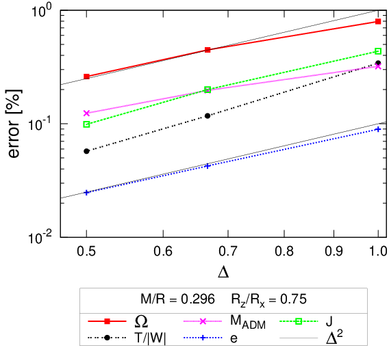
As discussed in the section II.3.5, our choice of finite difference approximations is second order. The rate of convergence of our code is checked using different resolutions, whose setups of coordinate grids are shown in Table 2. The grid spacing of each coordinate $(\Delta r,\Delta\theta,\Delta\phi)$ is proportionally scaled as $2/3$ , $3/4$ , $2/3$ , $3/4$ , from type I-1 to I-5. Here, we show the results of the convergence test with respect to the resolutions, fixing the maximum number of multipoles $L$ as shown in Table 2. ²² 2 For the convergence tests with respect to the order of the Legendre expansion, see [28].

When a sufficient number of multipoles is kept, the differences between numerically computed quantities with different resolutions and their exact value are written

f_{{\rm I}\mbox{-}i}\,-\,f_{\rm exact}\,=\,A\Delta^{n}_{{\rm I}\mbox{-}i}+{O}(\Delta^{n+1}_{{\rm I}\mbox{-}i})

(43)

where $f_{{\rm I}\mbox{-}i}$ ( $i=1,\cdots,5$ ) is a quantity computed using one of the resolution types ${\rm I}\mbox{-}i$ in Table 2, $f_{\rm exact}$ is its exact value, $\Delta_{{\rm I}\mbox{-}i}$ represents the grid spacing associated with the type ${\rm I}\mbox{-}i$ setup, and $A$ is a constant. Then, keeping the leading term, differences between different resolutions become

f_{{\rm I}\mbox{-}k}\,-\,f_{{\rm I}\mbox{-}i}\,=\,A\left[\left(\frac{\Delta_{{\rm I}\mbox{-}k}}{\Delta_{{\rm I}\mbox{-}i}}\right)^{n}-1\right]\Delta^{n}_{{\rm I}\mbox{-}i}.

(44)

To see the order $n$ in a log-log plot, we select the combinations of different resolutions that give the same ratio $\Delta_{{\rm I}\mbox{-}k}/\Delta_{{\rm I}\mbox{-}i}$ , and in our choice, these are $f_{{\rm I}\mbox{-}3}-f_{{\rm I}\mbox{-}1}$ , $f_{{\rm I}\mbox{-}4}-f_{{\rm I}\mbox{-}2}$ , and $f_{{\rm I}\mbox{-}5}-f_{{\rm I}\mbox{-}3}$ . In Fig.1, these combinations normalized by $f_{{\rm I}\mbox{-}5}$ of selected quantities are plotted against the grid spacing, where $\Delta$ represents the grid spacing in arbitrary units. It is clearly seen that the local quantities, here $\Omega$ and $e$ , converge to ${O}(\Delta^{2})$ , and that integral (global) quantities also approach second order convergence as the resolution increases.

We also checked the convergence with the different sets of resolutions type II-1, 2 and 3. These setups have fewer grid points in the angular coordinates $\theta$ and $\phi$ . We found that the highest resolution type II-3 agrees well with the results of the higher resolutions of type I-4 or 5 for the axisymmetric solutions.

Refer to caption — Figure 1: The convergence of quantities, $\Omega$ , $M_{\rm ADM}$ , $J$ , $T/|W|$ and $e:=\sqrt{1-({\bar{R}}_{z}/{\bar{R}}_{x})^{2}}$ (in the proper length) for the model with $n=0.5$ , $M/R=0.296$ and axis ratio in the coordinate length $R_{z}/R_{x}=0.75$ . Normalized differences $|(f_{{\rm I}\mbox{-}5}-f_{{\rm I}\mbox{-}3})/f_{{\rm I}\mbox{-}5}|$ , $|(f_{{\rm I}\mbox{-}4}-f_{{\rm I}\mbox{-}2})/f_{{\rm I}\mbox{-}5}|$ , and $|(f_{{\rm I}\mbox{-}3}-f_{{\rm I}\mbox{-}1})/f_{{\rm I}\mbox{-}5}|$ discussed in the text are plotted from left to right for each quantity against the resolutions $\Delta_{{\rm I}\mbox{-}3}$ , $\Delta_{{\rm I}\mbox{-}2}$ , and $\Delta_{{\rm I}\mbox{-}1}$ , respectively. Black thin lines are proportional to $\Delta^{2}$ .

III.2 Triaxial solutions with $M/R=0.001$

We calculate triaxial sequences for small compactness $M/R=0.001$ , which is in the Newtonian regime, to check the value of $T/|W|$ at the bifurcation point of the triaxial sequence from the axisymmetric sequence. The triaxial and axisymmetric solution sequences for $n=0.3$ and $0.5$ are plotted in Fig. 2. Extrapolating the triaxial sequences to corresponding axisymmetric sequences, values at the branch points are determined approximately as $(\Omega M,T/|W|)=(1.735\times 10^{-5},0.134)$ and $(1.763\times 10^{-5},0.135)$ for $n=0.3$ and $0.5$ , respectively. This value may be compared with the Newtonian results such as the ellipsoidal approximation $T/|W|=0.138$ for $n=0.5$ [5].

IV Triaxial solutions

IV.1 Accuracy of the sequences of solutions

Triaxially deformed solutions are calculated for selected values of the polytropic index, $n=0.3$ and $0.5$ . Models with $M/R=0.001,0.1,0.14,0.2$ are calculated for $n=0.3$ and with $M/R=0.1,0.12,0.14$ for $n=0.5$ .

We noticed that it is necessary to increase the numbers of grid points as much as in type I-5 in Table 2 to have a smoothly changing sequence of triaxial solutions. For lower resolutions, the sequences appear to be less smooth especially for the plot of $T/|W|$ and for the part of the sequences closer to axisymmetric solutions. One of the reasons for this may be that, when one compares neighboring solutions of deformed sequences for mass, binding energy, or angular momentum, the change in these quantities for triaxial sequences is much smaller than that for axially symmetric sequences of about the same amount of deformation.

IV.2 Properties of the triaxial sequences

As a sample of calculated solutions, the density contours in the $xy$ , $xz$ , and $yz$ planes and the surface plot of the model with parameters $n=0.5$ and $M/R=0.2$ and the largest deformation are presented in Fig.3. The solution corresponds to the last row of data shown in Table 5 in Appendix B.

In Figs. 4 and 5, $T/|W|$ and $\Omega M$ are plotted for $n=0.3$ and $0.5$ respectively, against the eccentricity for the constant rest mass sequences shown in the same Table 5. For uniformly rotating Newtonian polytropes, $T/|W|$ at the bifurcation point weakly depends on the difference of the EOS parameter, the polytropic index, whose value is about $T/|W|\sim 0.14$ . For highly differential rotations, $T/|W|$ may vary largely [18, 34]. The definitions of $T$ and $W$ in general relativity are given in Appendix A.

Our results for the solution sequences of uniformly rotating relativistic polytropes with $n=0.3$ and $0.5$ suggest that the value of $T/|W|$ at the bifurcation point strongly depends on compactness $M/R$ . In Table 4, approximate values of quantities at the bifurcation point of each model are shown, which are evaluated by linearly extrapolating the triaxial sequence to the corresponding axisymmetric sequence. The value of $T/|W|$ at the bifurcation point becomes $\sim 0.169$ for the compact model $M/R=0.2$ , $n=0.3,$ and it will certainly increase for a more compact sequence.

As seen in the plot of Fig. 5, the triaxial solution sequence for $n=0.5$ becomes shorter as $M/R$ increases. In fact, we were not able to find a triaxial solution sequence for $M/R=0.2$ ; the triaxial sequence may disappear at a certain value of $M/R$ between 0.14-0.2. We discuss an interesting consequence of the disappearance of triaxial sequences for high compactness in the last section.

$n$	$M/R$	$R_{x}$	$R_{z}/R_{x}$	$\epsilon_{c}$	$\Omega$	$M_{\rm ADM}$	$J$	$T/\|W\|$	$I$	$Z_{\rm p}$
0.3	0.1	$0.3226$ $(0.3718)$	$0.5634$ $(0.5693)$	$0.3888$	$0.6529$	$2.8444\times 10^{-2}$	$8.794\times 10^{-4}$	$0.1507$	$1.347\times 10^{-3}$	$0.1328$
0.3	0.14	$0.3435$ $(0.4220)$	$0.5531$ $(0.5619)$	$0.4445$	$0.7161$	$4.4203\times 10^{-2}$	$1.903\times 10^{-3}$	$0.1578$	$2.657\times 10^{-3}$	$0.2019$
0.3	0.2	$0.3561$ $(0.4860)$	$0.5394$ $(0.5535)$	$0.5244$	$0.8063$	$6.9865\times 10^{-2}$	$4.351\times 10^{-3}$	$0.1688$	$5.395\times 10^{-3}$	$0.3311$
0.5	0.1	$0.5153$ $(0.5919)$	$0.5461$ $(0.5536)$	$0.2059$	$0.4391$	$4.2103\times 10^{-2}$	$1.913\times 10^{-3}$	$0.1493$	$4.356\times 10^{-3}$	$0.1281$
0.5	0.12	$0.5209$ $(0.6169)$	$0.5439$ $(0.5531)$	$0.2319$	$0.4698$	$5.2155\times 10^{-2}$	$2.753\times 10^{-3}$	$0.1519$	$5.861\times 10^{-3}$	$0.1594$
0.5	0.14	$0.5314$ $(0.6482)$	$0.5366$ $(0.5482)$	$0.2581$	$0.4995$	$6.2304\times 10^{-2}$	$3.734\times 10^{-3}$	$0.1542$	$7.476\times 10^{-3}$	$0.1932$

Table 4: Quantities at the point of bifurcation of triaxial sequences from axisymmetric sequences. The polytropic index

n

and the compactness of the spherical star with the same rest mass

M/R

are the model parameters. Corresponding triaxial sequences are found in Table 5 in Appendix B. In the above,

R_{x}

is the equatorial radius, and

R_{z}/R_{x}

is the ratio of polar to the equatorial radius. Each has two values; one is measured in the coordinate length, and the other in parenthesis is in proper length defined in Eq.(55).

\epsilon_{c}

is the energy density at the center of the compact star,

\Omega

is the angular velocity. Definitions of

M_{\rm ADM}

J

T/|W|

, and

I

are found in Appendix A.

Z_{\rm p}

is the polar redshift. Dimensional quantities are shown in

G=c=\kappa=1

units.

V Discussion: proto-neutron star contraction

As a result of massive stellar core collapses, proto-neutron stars are formed and contract to more compact neutron stars within the time scale of cooling of a few tens of seconds [36]. Even for the small rotation rate of the collapsing stellar core, the ratio $T/|W|$ of the proto-neutron star becomes much higher than the value where the axisymmetric solution becomes secularly unstable against the viscosity driven $\ell=m=2$ bar mode instability [4, 5]. Therefore, uniformly rotating triaxial solutions discussed in this paper may describe a quasi-stationary model of proto-neutron star contraction in the range of $M/R\sim 0.1-0.2$ , assuming the following: (1) a certain mechanism of strong viscosity operates during the contraction, (2) the time scale rapid cooling is shorter than that of gravitational radiation reaction, (3) the effective polytropic (adiabatic) index $n$ $(\Gamma=1+1/n)$ of the EOS for the realistic neutron star matter is small (large) enough to allow uniformly rotating triaxial solutions, and (4) those triaxial solutions are dynamically stable.

Such an evolutionary track of a proto-neutron star contraction has been considered using a compressible ellipsoidal model³³ 3 In their work, changes in the entropy during the evolution is modeled by the changes in the adiabatic constant $\kappa$ of the polytropic EOS. [5]. Our results add two further important features to this. First, the sequences of triaxial solutions terminate at the maximally deformed models, at the mass-shedding limits, and the changes in ADM mass or total angular momentum are small along the triaxial sequences from the bifurcation points to the termination points, even for the stiffer EOS such as $n=0.3$ , as seen in Table 5; the triaxial sequences are not very long at all. Secondly, the triaxial sequences may become shorter and disappear as the compactness becomes larger for a relatively less stiff EOS such as $n=0.5$ .

The angular velocity near the braking limit is estimated as $\Omega M\sim(M/R)^{3/2}\sim(M/R)^{2}J/M^{2}$ . Therefore once the secular bar mode instability sets in, conserving $M$ and $J$ , the proto-neutron star evolves towards a maximally deformed triaxial configuration as it contracts, say, from $M/R\sim 0.1$ to $0.2$ . And then, it is likely that it always evolves along the sequence of maximally deformed configurations during the contraction as long as such triaxial solutions exist and are dynamically stable in the parameter region of the effective $\Gamma$ and $M/R$ . Excess angular momentum arising from contraction may be transported outward by mass ejected from the Lagrange point at the cusp of the longest semi-major axis. (Note that the time scale of the mass ejection may be that of cooling, which is much longer than the dynamical time scale.) Furthermore, if the effective $\Gamma$ satisfies $\Gamma\lesssim 3$ , the triaxial solution may disappear when the solution reaches a certain value of the compactness $M/R$ and higher. Dynamically stability of such uniformly rotating solutions are not known, but it is unlikely that the dynamical instability appears within such short triaxial sequences, along which the ratio $T/|W|$ is nearly constant.

It is estimated that the amplitude of gravitational wave (GW) signals from such objects may be detectable using the ground based laser interferometric detectors, if the source is within a few tens of Mpc [4, 18]. Detection of the persistent GW signals even after the proto-neutron star contraction phase suggests a large effective $\Gamma\gtrsim 3$ , while the shutdown of the signal during the contraction implies the relatively smaller $\Gamma\lesssim 3$ . Detection of such GW signal may set another constraint on the EOS parameter of high density matter. Source modeling for constructing the wave templates may be straightforward because one can concentrate on calculating the maximally deformed configurations. Our next plan is to include more realistic nuclear EOS in the code, then to estimate the gravitational wave amplitude for those EOSs that allow the triaxial solutions.

Acknowledgements.

We would like to thank John Friedman for discussions and warm encouragement. KU thanks Yoshiharu Eriguchi for discussions and for providing a reprint of PhD thesis by Tetsuo Nozawa, and Shin Yoshida for discussions. This work was supported by NSF grants No. PHY0071044, PHY0503366, NASA Grant No. NNG05GB99G, the Greek State Scholarships Foundation, and JSPS Grant-in-Aid for Scientific Research(C) 20540275.

Appendix A Formulas for mass and angular momentum

Definitions of the quantities shown in tables and figures that characterize each solution of a rotating relativistic star, and their expressions in terms of the metric potentials in the IWM formulation, are summarized in this Appendix.

The rest mass of the star $M_{0}$ is written as

M_{0}\,:=\,\int_{\Sigma}\rho\,u^{\alpha}dS_{\alpha}\,=\,\int_{\Sigma}\rho u^{t}\alpha\psi^{6}\sqrt{f}d^{3}x

(45)

where $dS_{\alpha}=\nabla_{\alpha}t\sqrt{-g}d^{3}x$ and $\sqrt{-g}d^{3}x\,=\,\alpha\psi^{6}\sqrt{f}d^{3}x$ $\,=\,\alpha\psi^{6}r^{2}\sin\theta drd\theta d\phi$ .

The ADM mass $M_{\rm ADM}$ becomes

$\displaystyle M_{\rm ADM}$	$\displaystyle:=$	$\displaystyle\frac{1}{16\pi}\int_{\infty}\left(f^{ac}f^{bd}-f^{ab}f^{cd}\right){\raise 4.30554pt\hbox{${}^{\ \circ}$}}\!\!\!\!\!D_{b}\gamma_{cd}\,dS_{a}$
	$\displaystyle=$	$\displaystyle-\frac{1}{2\pi}\int_{\infty}{\raise 4.30554pt\hbox{${}^{\ \circ}$}}\!\!\!\!\!D{}^{a}\psi\,d{\raise 4.30554pt\hbox{${}^{\ \circ}$}}\!\!\!\!\!S_{a}\,=\,-\frac{1}{2\pi}\int_{\Sigma}{\raise 4.30554pt\hbox{${}^{\ \circ}$}}\!\!\!\!\Delta\psi\,d{\raise 4.30554pt\hbox{${}^{\ \circ}$}}\!\!\!\!\!S$
	$\displaystyle=$	$\displaystyle\frac{1}{2\pi}\int_{\Sigma}\left[\,\frac{1}{8}\psi^{5}\tilde{A}_{ab}\tilde{A}^{ab}\,+\,2\pi\psi^{5}\rho_{\rm H}\,\right]\sqrt{f}d^{3}x,$

where $d{\raise 4.30554pt\hbox{${}^{\ \circ}$}}\!\!\!\!\!S_{a}=\nabla_{a}r\sqrt{f}d^{2}x$ and $d{\raise 4.30554pt\hbox{${}^{\ \circ}$}}\!\!\!\!\!S\,=\,\sqrt{f}d^{3}x$ , and $dS_{a}$ coincides with $d{\raise 4.30554pt\hbox{${}^{\ \circ}$}}\!\!\!\!\!S_{a}$ at spatial infinity.

The Komar mass associated with a timelike Killing field $t^{\alpha}$ is written

	$\displaystyle M_{\rm K}$	$\displaystyle:=$	$\displaystyle-\frac{1}{4\pi}\int_{\infty}\nabla^{\alpha}\,t^{\beta}\,dS_{{\alpha\beta}}\,=\,-\frac{1}{4\pi}\int_{\Sigma}R^{\alpha}\!{}_{\beta}t^{\beta}\,dS_{\alpha}$		(47)
		$\displaystyle=$	$\displaystyle\int_{\Sigma}\left(\,2T^{\alpha}\!{}_{\beta}-Tg^{\alpha}\!_{\beta}\,\right)\,t^{\beta}\,dS_{\alpha},$		(47)

and, in the IWM formulation, we have

M_{\rm K}=\int_{\Sigma}\left[\,\alpha\left(\rho_{\rm H}+S\right)-2j_{a}\beta^{a}\,\right]\psi^{6}\sqrt{f}d^{3}x,

(48)

where $dS_{\alpha}=n_{\alpha}\sqrt{\gamma}d^{3}x$ was used. The above derivation holds if the global timelike Killing field exists. For the spacetime of a triaxially deformed rotating star, no such timelike Killing field exists. Instead, an asymptotic Komar mass can be written

$\displaystyle M_{\rm K}$	$\displaystyle:=$	$\displaystyle-\frac{1}{4\pi}\int_{\infty}\nabla^{\alpha}t^{\beta}\,dS_{{\alpha\beta}}\,=\,\frac{1}{4\pi}\int_{\infty}D^{a}\alpha\,dS_{a}$
	$\displaystyle=$	$\displaystyle\frac{1}{4\pi}\int_{\Sigma}\Delta\alpha\,d\Sigma$
	$\displaystyle=$	$\displaystyle\frac{1}{4\pi}\int_{\Sigma}\left[\,\alpha\tilde{A}_{ab}\tilde{A}^{ab}+4\pi\alpha\left(\rho_{\rm H}+S\right)\,\right]\psi^{6}\sqrt{f}d^{3}x.$

In [35], we have derived sufficient conditions of the fall off of the 3-metric $\gamma_{ab}$ and extrinsic curvature $K_{ab}$ and their time derivative for the $M_{\rm ADM}=M_{\rm K}$ relation to be satisfied. In the IWM formulation the fall off of each field is sufficiently fast to have the equality. And also in this case, the above two definitions for $M_{\rm K}$ agree.

The total angular momentum calculated in the asymptotics is written

$\displaystyle J$	$\displaystyle:=$	$\displaystyle-\frac{1}{8\pi}\int_{\infty}\pi^{a}{}_{b}\phi^{b}\,dS_{a}\,=\,\frac{1}{8\pi}\int_{\infty}K^{a}{}_{b}\phi^{b}\,dS_{a}$	(50)
	$\displaystyle=$	$\displaystyle\frac{1}{8\pi}\int_{\Sigma}D_{a}(K^{a}{}_{b}\phi^{b})\,dS$	(50)
	$\displaystyle=$	$\displaystyle\frac{1}{8\pi}\int_{\Sigma}8\pi j_{a}\phi^{a}\psi^{6}\sqrt{f}d^{3}x.$	(51)

The relativistic analog of the kinetic energy $T$ is defined by

T:=\frac{1}{2}\int\Omega dJ,

(52)

therefore, for uniform rotation we have $T=\frac{1}{2}\Omega J$ . Also the relativistic analog of the gravitational potential energy $W$ is defined by

W:=M_{\rm p}+T-M_{\rm ADM},

(53)

where $M_{\rm p}$ is the proper mass defined by

M_{\rm p}\,:=\,\int_{\Sigma}\epsilon\,u^{\alpha}dS_{\alpha}\,=\,\int_{\Sigma}\epsilon u^{t}\alpha\psi^{6}\sqrt{f}d^{3}x.

(54)

The proper length of the semi-major axis along the $x$ direction is written

\displaystyle\bar{R}_{x}=\int_{0}^{R_{x}}\psi^{2}dx,

(55)

where $R_{x}$ is the coordinate length of the same axis. The proper lengths along the $y$ or $z$ directions are calculated using the same formula, replacing $x$ by $y$ or $z$ respectively.

In the above, the source terms of the field equations, $\rho_{\rm H}$ , $j_{a}$ , and $S$ , are obtained from the stress energy tensor. We write down the projection of the stress tensor in terms of elementary fluid variables and metric potentials. The 4-velocity for the corotational flow $u^{\alpha}=u^{t}k^{\alpha}$ is decomposed with respect to the foliation $\Sigma_{t}$ as

	$\displaystyle u^{\alpha}n_{\alpha}$	$\displaystyle=$	$\displaystyle-\alpha u^{t}$		(56)
	$\displaystyle u^{\alpha}\gamma_{\alpha a}$	$\displaystyle=$	$\displaystyle u^{t}\omega_{a}.$		(57)

Using these relations, the source terms of the field equations become

$\displaystyle\rho_{\rm H}\,$	$\displaystyle:=$	$\displaystyle\,T_{\alpha\beta}n^{\alpha}n^{\beta}\,=\,h\rho(\alpha u^{t})^{2}-p,$	(58)
$\displaystyle j_{a}\,$	$\displaystyle:=$	$\displaystyle\,-T_{\alpha\beta}\gamma_{a}\!{}^{\alpha}n^{\beta}\,=\,h\rho\alpha(u^{t})^{2}\psi^{4}\tilde{\omega}_{a},$	(59)
$\displaystyle S\,$	$\displaystyle:=$	$\displaystyle\,T_{\alpha\beta}\gamma^{{\alpha\beta}}\,=\,h\rho\big[(\alpha u^{t})^{2}-1\big]+3\,p,$	(60)

where $\tilde{\omega}_{a}\,:=\,f_{ab}\omega^{b}\,=\,f_{ab}(\beta^{b}+\Omega\phi^{b})\,=\,\tilde{\beta}_{a}+\Omega\tilde{\phi}_{a}$ .

Throughout the paper we use units such that $G=c=\kappa=1$ . The latter equality is implemented by renormalizing the length and mass scales as

\bar{R}\,:=\,\kappa^{-n/2}R,\qquad\bar{M}\,:=\,\kappa^{-n/2}M.

(61)

respectively. Angular momentum and angular frequency are respectively normalized as

\bar{J}\,:=\,\kappa^{-n}J,\qquad\bar{\Omega}\,:=\,\kappa^{n/2}\Omega.

(62)

We omit the bars over these quantities in the main text.

Appendix B Selected solution sequences

Sequences of triaxially deformed solutions of the compact star were calculated for the following parameters: the polytropic index $n=0.3$ with compactness $M/R=0.1,0.14,0.2$ , and the polytropic index $n=0.5$ with compactness $M/R=0.1,0.12,0.14$ . Quantities, most of which are defined in Appendix A are tabulated in Table 5. This data is plotted in Fig.4 and 5.

$n=0.3\quad$ $M/R=0.10\quad$ $M_{0}=2.9908\times 10^{-2}\quad$ $M=2.8116\times 10^{-2}\quad$
$R_{x}$	$R_{y}/R_{x}$	$R_{z}/R_{x}$	$\epsilon_{c}$	$\Omega$	$M_{\rm ADM}$	$J$	$T/\|W\|$	$I$	$Z_{p}$
$0.3367$ $(0.3875)$	$0.9375$ $(0.9389)$	$0.5423$ $(0.5485)$	$0.3884$	$0.6504$	$2.8446\times 10^{-2}$	$8.845\times 10^{-4}$	$0.1512$	$1.360\times 10^{-3}$	$0.1327$
$0.3461$ $(0.3981)$	$0.8906$ $(0.8929)$	$0.5273$ $(0.5337)$	$0.3882$	$0.6493$	$2.8447\times 10^{-2}$	$8.871\times 10^{-4}$	$0.1515$	$1.366\times 10^{-3}$	$0.1326$
$0.3567$ $(0.4098)$	$0.8438$ $(0.8470)$	$0.5115$ $(0.5181)$	$0.3880$	$0.6475$	$2.8449\times 10^{-2}$	$8.909\times 10^{-4}$	$0.1518$	$1.376\times 10^{-3}$	$0.1326$
$0.3645$ $(0.4185)$	$0.8125$ $(0.8164)$	$0.5008$ $(0.5075)$	$0.3878$	$0.6457$	$2.8450\times 10^{-2}$	$8.937\times 10^{-4}$	$0.1520$	$1.384\times 10^{-3}$	$0.1325$
$0.3775$ $(0.4330)$	$0.7656$ $(0.7704)$	$0.4833$ $(0.4902)$	$0.3874$	$0.6423$	$2.8453\times 10^{-2}$	$8.992\times 10^{-4}$	$0.1524$	$1.400\times 10^{-3}$	$0.1323$
$0.3875$ $(0.4441)$	$0.7344$ $(0.7397)$	$0.4707$ $(0.4778)$	$0.3871$	$0.6397$	$2.8455\times 10^{-2}$	$9.043\times 10^{-4}$	$0.1528$	$1.414\times 10^{-3}$	$0.1322$
$0.3987$ $(0.4564)$	$0.7031$ $(0.7091)$	$0.4574$ $(0.4647)$	$0.3867$	$0.6366$	$2.8458\times 10^{-2}$	$9.095\times 10^{-4}$	$0.1532$	$1.429\times 10^{-3}$	$0.1320$
$0.4188$ $(0.4784)$	$0.6562$ $(0.6633)$	$0.4355$ $(0.4433)$	$0.3863$	$0.6318$	$2.8461\times 10^{-2}$	$9.171\times 10^{-4}$	$0.1536$	$1.452\times 10^{-3}$	$0.1318$
$n=0.3\quad$ $M/R=0.14\quad$ $M_{0}=4.7471\times 10^{-2}\quad$ $M=4.3417\times 10^{-2}\quad$
$R_{x}$	$R_{y}/R_{x}$	$R_{z}/R_{x}$	$\epsilon_{c}$	$\Omega$	$M_{\rm ADM}$	$J$	$T/\|W\|$	$I$	$Z_{p}$
$0.3619$ $(0.4435)$	$0.9219$ $(0.9245)$	$0.5291$ $(0.5385)$	$0.4441$	$0.7124$	$4.4208\times 10^{-2}$	$1.913\times 10^{-3}$	$0.1581$	$2.686\times 10^{-3}$	$0.2017$
$0.3763$ $(0.4603)$	$0.8594$ $(0.8639)$	$0.5089$ $(0.5187)$	$0.4439$	$0.7103$	$4.4210\times 10^{-2}$	$1.919\times 10^{-3}$	$0.1582$	$2.702\times 10^{-3}$	$0.2016$
$0.3889$ $(0.4751)$	$0.8125$ $(0.8185)$	$0.4924$ $(0.5026)$	$0.4436$	$0.7077$	$4.4213\times 10^{-2}$	$1.927\times 10^{-3}$	$0.1584$	$2.722\times 10^{-3}$	$0.2014$
$0.3985$ $(0.4861)$	$0.7812$ $(0.7882)$	$0.4807$ $(0.4911)$	$0.4434$	$0.7056$	$4.4216\times 10^{-2}$	$1.933\times 10^{-3}$	$0.1586$	$2.739\times 10^{-3}$	$0.2012$
$0.4091$ $(0.4984)$	$0.7500$ $(0.7579)$	$0.4684$ $(0.4792)$	$0.4431$	$0.7032$	$4.4220\times 10^{-2}$	$1.940\times 10^{-3}$	$0.1587$	$2.758\times 10^{-3}$	$0.2010$
$0.4215$ $(0.5127)$	$0.7188$ $(0.7278)$	$0.4548$ $(0.4659)$	$0.4429$	$0.7007$	$4.4223\times 10^{-2}$	$1.947\times 10^{-3}$	$0.1589$	$2.778\times 10^{-3}$	$0.2008$
$0.4364$ $(0.5296)$	$0.6875$ $(0.6978)$	$0.4395$ $(0.4513)$	$0.4427$	$0.6983$	$4.4226\times 10^{-2}$	$1.952\times 10^{-3}$	$0.1590$	$2.796\times 10^{-3}$	$0.2007$
$n=0.3\quad$ $M/R=0.20\quad$ $M_{0}=7.7530\times 10^{-2}\quad$ $M=6.7804\times 10^{-2}$
$R_{x}$	$R_{y}/R_{x}$	$R_{z}/R_{x}$	$\epsilon_{c}$	$\Omega$	$M_{\rm ADM}$	$J$	$T/\|W\|$	$I$	$Z_{p}$
$0.3745$ $(0.5091)$	$0.9219$ $(0.9262)$	$0.5162$ $(0.5313)$	$0.5242$	$0.8036$	$6.9868\times 10^{-2}$	$4.360\times 10^{-3}$	$0.1687$	$5.426\times 10^{-3}$	$0.3308$
$0.3819$ $(0.5184)$	$0.8906$ $(0.8967)$	$0.5064$ $(0.5219)$	$0.5242$	$0.8026$	$6.9869\times 10^{-2}$	$4.362\times 10^{-3}$	$0.1686$	$5.435\times 10^{-3}$	$0.3306$
$0.3945$ $(0.5343)$	$0.8438$ $(0.8524)$	$0.4905$ $(0.5066)$	$0.5241$	$0.8008$	$6.9870\times 10^{-2}$	$4.369\times 10^{-3}$	$0.1686$	$5.456\times 10^{-3}$	$0.3305$
$0.4227$ $(0.5691)$	$0.7656$ $(0.7791)$	$0.4584$ $(0.4762)$	$0.5240$	$0.7968$	$6.9873\times 10^{-2}$	$4.380\times 10^{-3}$	$0.1683$	$5.498\times 10^{-3}$	$0.3300$
$n=0.5\quad$ $M/R=0.10\quad$ $M_{0}=4.4113\times 10^{-2}\quad$ $M=4.1580\times 10^{-2}$
$R_{x}$	$R_{y}/R_{x}$	$R_{z}/R_{x}$	$\epsilon_{c}$	$\Omega$	$M_{\rm ADM}$	$J$	$T/\|W\|$	$I$	$Z_{p}$
$0.5407$ $(0.6197)$	$0.9219$ $(0.9243)$	$0.5238$ $(0.5319)$	$0.2059$	$0.4380$	$4.2103\times 10^{-2}$	$1.915\times 10^{-3}$	$0.1492$	$4.373\times 10^{-3}$	$0.1281$
$0.5580$ $(0.6387)$	$0.8750$ $(0.8789)$	$0.5079$ $(0.5163)$	$0.2059$	$0.4373$	$4.2104\times 10^{-2}$	$1.917\times 10^{-3}$	$0.1491$	$4.384\times 10^{-3}$	$0.1280$
$0.5716$ $(0.6536)$	$0.8438$ $(0.8486)$	$0.4959$ $(0.5047)$	$0.2059$	$0.4367$	$4.2104\times 10^{-2}$	$1.919\times 10^{-3}$	$0.1491$	$4.393\times 10^{-3}$	$0.1280$
$0.5880$ $(0.6715)$	$0.8125$ $(0.8185)$	$0.4823$ $(0.4914)$	$0.2059$	$0.4361$	$4.2104\times 10^{-2}$	$1.920\times 10^{-3}$	$0.1490$	$4.402\times 10^{-3}$	$0.1279$
$n=0.5\quad$ $M/R=0.12\quad$ $M_{0}=5.5171\times 10^{-2}\quad$ $M=5.1345\times 10^{-2}$
$R_{x}$	$R_{y}/R_{x}$	$R_{z}/R_{x}$	$\epsilon_{c}$	$\Omega$	$M_{\rm ADM}$	$J$	$T/\|W\|$	$I$	$Z_{p}$
$0.5508$ $(0.6500)$	$0.9219$ $(0.9250)$	$0.5188$ $(0.5289)$	$0.2319$	$0.4689$	$5.2155\times 10^{-2}$	$2.755\times 10^{-3}$	$0.1517$	$5.875\times 10^{-3}$	$0.1594$
$0.5693$ $(0.6708)$	$0.8750$ $(0.8800)$	$0.5021$ $(0.5127)$	$0.2319$	$0.4683$	$5.2156\times 10^{-2}$	$2.758\times 10^{-3}$	$0.1517$	$5.888\times 10^{-3}$	$0.1594$
$0.5934$ $(0.6976)$	$0.8281$ $(0.8352)$	$0.4818$ $(0.4932)$	$0.2319$	$0.4677$	$5.2156\times 10^{-2}$	$2.759\times 10^{-3}$	$0.1516$	$5.900\times 10^{-3}$	$0.1593$
$n=0.5\quad$ $M/R=0.14\quad$ $M_{0}=6.6547\times 10^{-2}\quad$ $M=6.1130\times 10^{-2}$
$R_{x}$	$R_{y}/R_{x}$	$R_{z}/R_{x}$	$\epsilon_{c}$	$\Omega$	$M_{\rm ADM}$	$J$	$T/\|W\|$	$I$	$Z_{p}$
$0.5410$ $(0.6591)$	$0.9688$ $(0.9703)$	$0.5282$ $(0.5401)$	$0.2580$	$0.4993$	$6.2304\times 10^{-2}$	$3.735\times 10^{-3}$	$0.1542$	$7.482\times 10^{-3}$	$0.1932$
$0.5630$ $(0.6843)$	$0.9062$ $(0.9109)$	$0.5077$ $(0.5203)$	$0.2580$	$0.4988$	$6.2305\times 10^{-2}$	$3.738\times 10^{-3}$	$0.1542$	$7.495\times 10^{-3}$	$0.1931$
$0.5771$ $(0.7003)$	$0.8750$ $(0.8813)$	$0.4954$ $(0.5085)$	$0.2580$	$0.4984$	$6.2306\times 10^{-2}$	$3.740\times 10^{-3}$	$0.1542$	$7.505\times 10^{-3}$	$0.1931$

Table 5: Quantities for the constant rest mass Jacobi-like triaxial sequences.

M_{0}

is the rest mass of each sequence, and

M

is the gravitational mass of the spherical star having the same

M_{0}

. In the definition of the compactness,

R

is the Schwartzschild radius of the spherical star. Tabulated quantities are the same as Table 4, except for

R_{x}

, which is the semi-major radius along the

x

-axis, and

R_{y}

, the semi-major radius along the

x

-axis. Dimensional quantities are shown in

G=c=\kappa=1

References

- [1] S. Woosley, and T. Janka, Nature Physics 1, 147 (2005); F.A. Rasio, and S.L.Shapiro, Class. Quantum. Grav. 16, R1 (1999); T.W. Baumgarte, and S.L. Shapiro, Physics Reports 376, 41 (2003); L.Bildsten, ApJ 501, L89 (1998); A.L. Watts, B. Krishnan, L. Bildsten, B.F. Schutz, arXiv:0803.4097.
- [2] S. Chandrasekhar, “Ellipsoidal Figures of Equilibrium”, New Haven: Yale University Press.
- [3] S. Chandrasekhar, Phys. Rev. Letters 24, 611 (1970); B. Miller, ApJ 181, 497 (1973); S. L. Detweiler, and L. Lindblom, ApJ 213, 193 (1977); L. Lindblom, S. L. Detweiler, ApJ 211, 565 (1977).
- [4] D. Lai, and S. L. Shapiro, ApJ 442, 259 (1995).
- [5] S. L. Shapiro, Astrophys. J. 613, 1213 (2004).
- [6] e.g., J. L. Houser and J. M. Centrella, Phys. Rev. D 54, 7278 (1996); K. C. B. New, J. M. Centrella and J. E. Tohline, Phys. Rev. D 62, 064019 (2000); J. D. Brown, Phys. Rev. D 62, 084024 (2000); M. Saijo, M. Shibata, T. W. Baumgarte and S. L. Shapiro, Astrophys. J. 548, 919 (2001); M. Shibata, S. Karino and Y. Eriguchi, Mon. Not. Roy. Astron. Soc. 334, L27 (2002); M. Shibata, S. Karino and Y. Eriguchi, Mon. Not. Roy. Astron. Soc. 343, 619 (2003); M. Shibata and S. Karino, Phys. Rev. D 70, 084022 (2004);
- [7] M. Shibata and Y. i. Sekiguchi, Phys. Rev. D 71, 024014 (2005).
- [8] e.g., M. Shibata and K. Uryū, Phys. Rev. D 61, 064001 (2000); M. Shibata and K. Uryū, Prog. Theor. Phys. 107, 265 (2002); M. Shibata, K. Taniguchi and K. Uryū, Phys. Rev. D 68, 084020 (2003); M. Shibata, K. Taniguchi and K. Uryū, Phys. Rev. D 71, 084021 (2005); Y. T. Liu, S. L. Shapiro, Z. B. Etienne and K. Taniguchi, arXiv:0803.4193 [astro-ph].
- [9] R.A. James, Astrophys. J., 140, 552, (1964).
- [10] N. Stergioulas, ”Rotating Stars in Relativity”, Living Rev. Relativity 6, (2003), http://www.livingreviews.org/lrr-2003-3
- [11] J. L. Friedman, J. R. Ipser, and L. Parker, Astrophys. J. 304, 115 (1986).
- [12] F. Douchin, and P. Haensel, A&A 380, 151 (2001); P. Haensel, and A. Y. Potekhin, A&A 428, 191 (2004).
- [13] T. Nozawa, “Quasi-stationary states of three dimensional stars in general relativity”, PhD thesis, University of Tokyo, (1997).
- [14] S.L. Shapiro, and S. Zane, Astrophys. J., 460, 379-389, (1996); T. Di Girolamo, and M. Vietri, Astrophys. J., 581, 519-549, (2002).
- [15] S. Bonazzola, J. Frieben, and E. Gourgoulhon, Astrophys. J., 460, 379, (1996); S. Bonazzola, J. Frieben, and E. Gourgoulhon, Astron. Astrophys., 331, 280, (1998).
- [16] N. Stergioulas, and J. L. Friedman, Astrophys. J. 492, 301 (1998).
- [17] D. Gondek-Rosinska, and E. Gourgoulhon, Phys. Rev. D 66, 044021, (2002); D. Gondek-Rosinska, E. Gourgoulhon, and P. Haensel, Astron. Astrophys., 412, 777 (2003).
- [18] M. Saijo, and E. Gourgoulhon, Phys. Rev. D74, 084006 (2006).
- [19] D. Skinner, and L. Lindblom, Astrophys. J., 461, 920, (1996).
- [20] S. Yoshida, and Y. Eriguchi, Astrophys. J. 490, 779 (1997).
- [21] J. Isenberg, Waveless Approximation Theories of Gravity, preprint (1978), University of Maryland; J. Isenberg and J. Nester, in General Relativity and Gravitation Vol.1, edited by A. Held, (Plenum Press, New York 1980).
- [22] J. R. Wilson and G. J. Mathews, in Frontiers in Numerical Relativity, ed. C.R. Evans, L.S. Finn and D.W. Hobill (Cambridge University Press, Cambridge, England, 1989), p.306.
- [23] G. B. Cook, S. L. Shapiro, and S. A. Teukolsky Phys. Rev. D 53, 5533 (1996).
- [24] W. Kley, and G. Schäfer, Phys. Rev. D 60, 027501 (1999); A. Garat, and R. H. Price, Phys.Rev. D 61, 124011 (2000).
- [25] F. Usui, K. Uryū and Y. Eriguchi, Phys. Rev. D 61, 024039 (2000)
- [26] K. Oohara, T. Nakamura and M. Shibata, Prog. Theor. Phys. Suppl. 128, 183 (1997); P. Grandclément, S. Bonazzola, E. Gourgoulhon, and J.-A. Marck, Journal of Computational Physics, 170, 231 (2001).
- [27] K. Uryū and Y. Eriguchi, Phys. Rev. D. 61, 124023 (2000); K. Uryū, M. Shibata and Y. Eriguchi, Phys. Rev. D. 62, 104015 (2000); K. Uryū, F. Limousin, J. L. Friedman, E. Gourgoulhon, and M. Shibata, Phys. Rev. Lett. 97, 171101 (2006);
- [28] A. A. Tsokaros, and K. Uryū, Phys. Rev. D75, 044026 (2007).
- [29] S. Bonazzola, E. Gourgoulhon, and J.-A. Marck, Journal of Computational and Applied Mathematics, 109, 433 (1999); S. Bonazzola, E. Gourgoulhon, and J.-A. Marck, Phys. Rev. D, 58, 104020 (1998); http://www.lorene.obspm.fr
- [30] J. P. Ostriker, and J. W.-K. Mark, Astrophys. J. 151, 1075 (1968).
- [31] H. Komatsu, Y. Eriguchi, and I. Hachisu, MNRAS 237, 355 (1989).
- [32] J. L. Friedman, K. Uryū, and M. Shibata, Phys. Rev. D 65, 064035 (2002); Erratum ibid. 70, 129904(E) (2004).
- [33] T. Nozawa, N. Stergioulas, E. Gourgoulhon, and Y. Eriguchi, Astron. Astrophys., suppl. ser. 132, 431 (1998).
- [34] S. Yoshida, S. Rezzolla, S. Karino, and Y. Eriguchi, Astrophys. J. 568, L41 (2002).
- [35] M. Shibata, K. Uryū, and J. L. Friedman, Phys. Rev. D 70, 044044 (2004); Erratum ibid. 70, 129901(E) (2004).
- [36] A. Burrows, and J. M. Lattimer, Astrophys. J. , 307, 178 (1986); J. A. Pons, A. W. Steiner, M. Prakash, and J. M. Lattimer, Phys. Rev. Lett. 86, 5223 (2001); J. A. Pons, J. A. Miralles, M. Prakash, and J. M. Lattimer, Astrophys. J. 553, 382 (2001); J. A. Pons, S. Reddy, M. Prakash, J. M. Lattimer, and J. A. Miralles, Astrophys. J. 513, 780 (1999).