Massive gravitons trapped inside a hypermonopole
Abstract
We propose a regular classical field theory realisation of the Dvali–Gabadadze–Porrati mechanism by considering our universe to be the four-dimensional core of a seven dimensional ’t Hooft–Polyakov hypermonopole. We show the existence of metastable gravitons trapped in the core. Their mass spectrum is discrete, positive definite, and computed for various values of the field coupling constants: the resulting Newton gravity law is seven-dimensional at small and large distances but can be made four-dimensional on intermediate length scales. There is no need of a cosmological constant in the bulk, the spacetime is asymptotically flat and of infinite volume in the extra-dimensions. Confinement is achieved through the local positive curvature of the extra-dimensions induced by the monopole-forming fields and for natural values of the coupling constants of order unity.
pacs
04.40.-b, 04.50.-h, 11.10.Kk, 98.80.CqI Introduction
Gravity occupies a central role in high energy physics and cosmology. On one hand, the unification of the fundamental interactions in the context of String Theory suggests that we may live in a more than four-dimensional world [1, 2]. On the other hand, the recent acceleration of our universe has been confirmed by different experiments and it is now a widely accepted important result of modern observational cosmology [3]. The idea that such an unexplained acceleration may be the signature of extra-dimensions has been intensively explored in the recent years [4, 5, 6]. In the Dvali–Gabadadze–Porrati (DGP) model, the extra-dimensions (bulk) may actually be non-compact and of infinite volume [7, 8]. Gravitons are reflected back onto our universe (brane) due to a different gravity coupling constant on the brane and in the bulk. The original DGP action in dimensions reads
| (1) |
where and are respectively the determinant and scalar curvature of the induced metric along our brane, while and are the corresponding quantities in the bulk. It has been shown that this model could actually explain the observed acceleration of the universe, although some works suggest that it may be spoiled by instabilities [9, 10, 11]. Although the form of Eq. (1) has been originally explained by quantum effects, “regularised models” have been proposed to justify it from a more classical and tractable point of view, free of instabilities. Such an approach has been explored in Refs [12, 13, 14] and shown to confine gravitons by explicitly choosing some profile for or . In a complete physical framework, both of these functions are however not free and it is not clear that the DGP mechanism could indeed appear in any classical system. This question is of crucial importance in order to assess the viability of both infinite volume extra-dimensions and instability-free DGP-like mechanism.
In this letter, we answer this question in the context of canonical classical field theory. Our approach is motivated by condensed matter physics: topological defects are a direct consequence of the symmetry breaking mechanism and can model smooth branes [15, 16, 17]. Assuming the space-time to be seven-dimensional, an spontaneous symmetry breaking in codimensions generically forms ’t Hooft–Polyakov hypermonopoles [18, 19]. In the following, we prove the existence of a DGP-like mechanism in the core (assumed to be our universe) of such a monopole.
Compared to lower dimensional defects [20], the existence of positively curved dimensional regions in the bulk is crucial to allow metastable gravitons to be trapped inside the core. Six is indeed the minimal number of spatial dimensions for which there exists a foliation of the extra-dimensions by two-dimensional positively curved surfaces. In order to allow for a varying Planck mass, we have for completeness included a dilaton having a mass in the Einstein frame. In the Jordan frame, the action associated with this system is
| (2) | ||||
where the dilaton potential reads . The Higgs field is in the triplet representation (). Its vacuum expectation value breaks into . The covariant derivatives enforce gauge invariance and incorporate the gauge fields ,
| (3) |
being the charge, while the field strength tensor is
| (4) |
As for the dimensional analysis, we have , , and .
II Background geometry
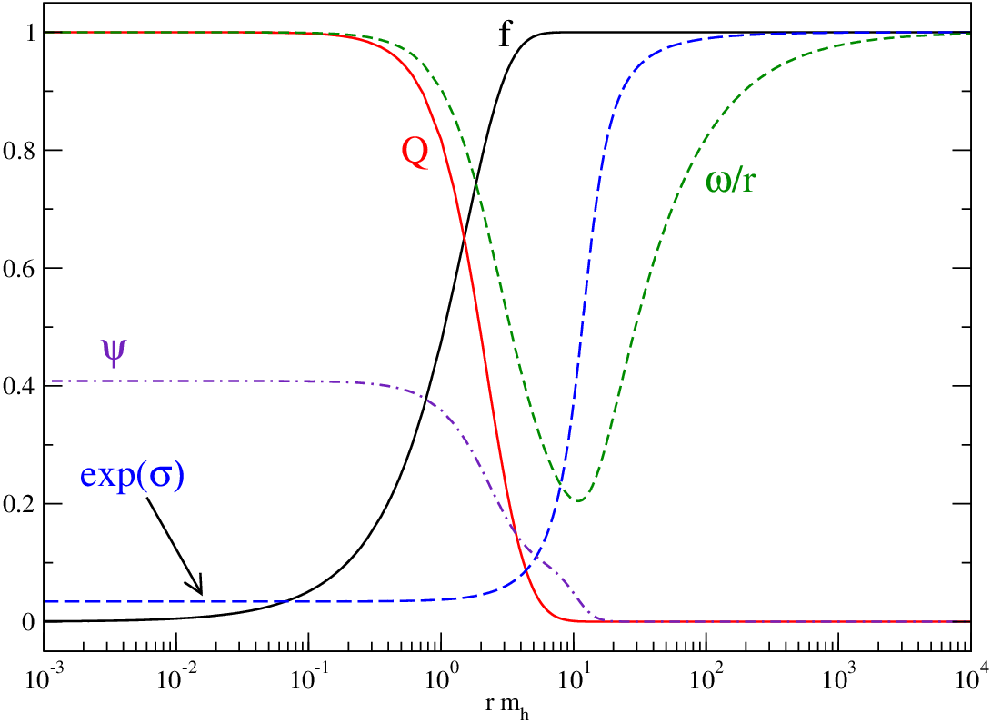

Static self-gravitating monopole configurations associated with the action (2) can be obtained by imposing isotropy in the extra-dimensions, plus Poincaré invariance along the four internal brane coordinates . Our ansatz for the metric is
| (5) |
where are spherical coordinates in the three extra-dimensions and . For the monopole-forming fields, the internal space of is mapped to the three extra-dimensions with a purely radial Higgs field
| (6) |
and winding gauge fields
| (7) |
the other components vanishing. Here, and are two dimensionless functions such that, far from the core, and to recover a Dirac monopole. In the core, regularity imposes and . Concerning the metric coefficients, the energy associated with the defect being finite and localised, we look for asymptotically flat spacetime, , and . Regularity in the core also imposes and .
The system of coupled non-linear differential equations obtained from the action (2) is of order ten and does not have any obvious analytical solution. Once the radial coordinate is expressed in unit of the Higgs Compton wavelength, the differential system is parametrised by three dimensionless parameters
| (8) |
where and are respectively the mass of the Higgs and gauge bosons. Under the above-mentioned boundary conditions, the numerical integration of the equations of motion is a challenging problem that has been overcome by using recent advances in the field [21]. We have found monopole solutions for almost any values of the above parameters; only when the stress energy becomes super-Planckian the system develops some singularities preventing the spacetime to be asymptotically flat. As can be seen in Fig. 1, the Higgs and gauge field profiles are typical of topological defect configurations while the dilaton is gravitationally trapped inside the core. The profile of traces the gravitational redshift: clocks are ticking differently inside and outside the monopole. More interesting is the profile of . Up to a factor, gives the area of the two-sphere of radius in the extra-dimensions. As can be seen in Fig. 1, there is a region at finite distance from the core where does no longer grow as but remains almost stationary: the extra-dimensions become cylindrically shaped. As we show in the next section, gravitons become resonant at these length scales and metastable from a four-dimensional point of view. Notice that the spacetime is non-compact and asymptotically Minkowski.
III Tensor fluctuations
We now consider the four-dimensional tensor perturbations around the previously computed background. The perturbed metric is given by Eq. (5) upon the replacement , where is a spacetime dependent transverse and traceless tensor. The linearised equations of motion for are obtained by expanding Eq. (2) at second order and have already been derived for an arbitrary number of extra-dimensions in Ref. [20]. Defining the dimensionless conformal radius and tensor as
| (9) |
the equation of motion for the spin-two fluctuations can be recast into
| (10) |
where the tensor indices have been omitted. Derivatives are with respect to , is the d’Alembertian along the brane, and
| (11) |
After a four-dimensional Fourier transform on the brane coordinates, and an expansion over the spherical harmonics in the angular extra-dimensions, we have in unit of the Higgs mass and . One immediately recognises in Eq. (10) the Schrödinger equation of a supersymmetric quantum mechanical system in a central potential [22]. The operator is the angular momentum, is the superpotential and plays the rôle of the energy. A subtlety is that our coordinate lies on the positive axis only. However, since must remain finite on the brane, Eq. (9) implies that should vanish in . Under this condition, and the usual normalisability at infinity, the differential operators remain regular enough to use the results of supersymmetric quantum mechanics. For , Eq. (10) is solved by the “ground state” which is however not normalisable asymptotically. The ground state of the superpartner potential is , which is not regular in . As a result, “supersymmetry” is broken and the spectrum is necessarily positive definite, : there is no massless mode neither tachyon on the brane.
Introducing the orthonormal basis of eigenfunctions , solutions of Eq. (10), such that
| (12) |
one can check that the retarded Green function for can be expanded as [23]
| (13) | ||||
Using the above equation together with Eq. (9), the tensor modes sourced by any transverse and traceless stress tensor are given by
| (14) | ||||
In order to gain some intuition on the previous expressions, let us first consider the case of a seven-dimensional flat spacetime. Setting everywhere, as well as , Eq. (10) can be integrated and the normalised modes are
| (15) |
Considering a “point-like” static source on the brane
| (16) |
we can explicitly integrate Eqs. (13) and (14) using the flat modes . Only the s-waves () have a non-vanishing contribution on the brane since for , one has . The four-dimensional integral over the momentum in Eq. (13), together with the denominator containing , is the classical retarded Yukawa propagator. After some calculations, one finally gets on the brane
| (17) | ||||
where . Using the expansion of the Bessel function, , the previous expression simplifies to
| (18) |
which is the standard linearised solution of the Einstein equations around a seven-dimensional Minkowski spacetime. Notice the power law dependence in spatial dimensions, as well as the factor which is times the surface of the unit –sphere, as one would have obtained from the Gauss law.

In the background geometry of the hypermonopole, the situation is nearly the same apart that the mode functions are now modified. As can be seen in Eq. (17), we need the values of the rescaled spectral density associated with s-waves on the brane . The tensor modes are then given by
| (19) |
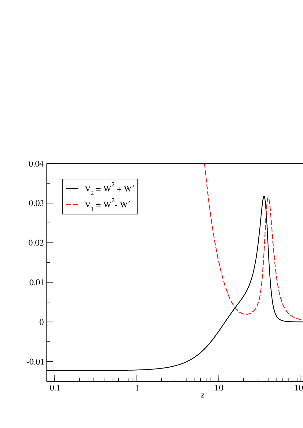
where stands for the forward Laplace transform evaluated at . From the monopole-forming fields computed in the previous section, we have plotted in Fig. 2 the potential and its superpartner. Since the spacetime is asymptotically flat, vanishes at infinity and there is not any bound state. However, (and also ) exhibits a barrier at the location of maximum curvature allowing metastable modes in the core. We have numerically solved the equation of motion (10) for these potentials and plotted in Fig. 3 the resulting spectral density. When this quantity is constant, gravity is purely seven-dimensional on the brane. This is the case for large, but also for low values of , as in the Gregory–Rubakov–Sibiryakov model [24].
Notice that the constant value of gives the effective gravitational coupling constant: here, it is different for large and low values of due to the dilaton condensation in the core as well as the gravitational redshift. In the intermediate range, is strongly peaked for particular values of : these are the resonant metastable modes. We have also numerically checked that there is not any bound state with , as expected from the supersymmetry arguments. Changing the background parameters , and affects the mass spectrum and the width or number of metastable modes can be easily adjusted. Lowering delocalises the gauge fields (in unit of the Higgs Compton wavelength) and the position of the barrier is pushed towards larger values of . Decreasing , or increasing , reduces the height of the barrier while changes its shape. Let us notice that if is too small, or too big, we do no longer observe resonances and this corresponds to the disappearance of the confining nest on . This is reminiscent with the properties of bound states in the case of broken supersymmetry.
To understand how these resonances realise the DGP mechanism, one can approximate them as Dirac distributions. Let us say we have one trapped graviton at a mass , then neglecting the smooth changes in the spectral density, where encodes how peaked the resonance is. The Laplace transform in Eq. (19) simplifies to
| (20) |
and four-dimensional gravity is recovered over the length scales , provided the mode is light enough . At small and large distances, seven dimensional gravity is recovered while in between we have even observed some fractional power dependencies. When more than one gravitons are trapped the situation becomes even more complex and the detailed analysis of these effects is left for a forthcoming work.
IV Conclusion
We proposed here a canonical classical field theory model which describes a seven-dimensional monopole, at the core of which gravitons get trapped. Their mass spectrum being positive definite, there are no instabilities for the tensor modes. This phenomenon turns out to be a natural way, in the context of field theory, to implement the DGP idea. The required field configurations can be obtained without fine-tuning from a dense set of coupling constant values of order unity. However, to obtain a four-dimensional gravity behaviour over a wide range of length scales, some amount of fine-tuning is certainly required to confine an almost massless mode. Notice that the smaller the graviton mass, the larger the effective four-dimensional Planck mass, possibly addressing the mass hierarchy problem. It would be interesting, if possible, to find a condensed matter system for which this mechanism could be experimentally explored.
Acknowledgements.
This work is supported by the Belgian Federal Office for Science, Technical and Cultural Affairs, under the Inter-university Attraction Pole grant P6/11.References
- [1] G. Nordström, Phys. Zeitschr. 15, 504 (1914).
- [2] J. Polchinski, String theory. An introduction to the bosonic string, Vol. I (Cambridge University Press, Cambridge, UK, 1998).
- [3] E. Komatsu et al. (WMAP) (2008), eprint 0803.0547.
- [4] N. Arkani-Hamed, S. Dimopoulos, and G. R. Dvali, Phys. Lett. B429, 263 (1998), eprint hep-ph/9803315.
- [5] L. Randall and R. Sundrum, Phys. Rev. Lett. 83, 4690 (1999), eprint hep-th/9906064.
- [6] C. Deffayet, G. R. Dvali, and G. Gabadadze, Phys. Rev. D65, 044023 (2002), eprint astro-ph/0105068.
- [7] G. R. Dvali, G. Gabadadze, and M. Porrati, Phys. Lett. B485, 208 (2000), eprint hep-th/0005016.
- [8] G. R. Dvali and G. Gabadadze, Phys. Rev. D63, 065007 (2001), eprint hep-th/0008054.
- [9] C. Deffayet, Phys. Lett. B502, 199 (2001), eprint hep-th/0010186.
- [10] C. Deffayet, G. Gabadadze, and A. Iglesias, JCAP 0608, 012 (2006), eprint hep-th/0607099.
- [11] R. Gregory, N. Kaloper, R. C. Myers, and A. Padilla, JHEP 10, 069 (2007), eprint 0707.2666.
- [12] M. Kolanovic, M. Porrati, and J.-W. Rombouts, Phys. Rev. D68, 064018 (2003), eprint hep-th/0304148.
- [13] M. Kolanovic, Phys. Rev. D67, 106002 (2003), eprint hep-th/0301116.
- [14] M. Shaposhnikov, P. Tinyakov, and K. Zuleta, Phys. Rev. D70, 104019 (2004), eprint hep-th/0411031.
- [15] T. Kibble, J. Phys. A9, 1387 (1976).
- [16] K. Akama, Lect. Notes Phys. 176, 267 (1982), eprint hep-th/0001113.
- [17] V. A. Rubakov and M. E. Shaposhnikov, Phys. Lett. B125, 136 (1983).
- [18] G. ’t Hooft, Nucl. Phys. B79, 276 (1974).
- [19] A. M. Polyakov, JETP Lett. 20, 194 (1974).
- [20] C. Ringeval and J.-W. Rombouts, Phys. Rev. D71, 044001 (2005), eprint hep-th/0411282.
- [21] J. R. Cash and F. Mazzia, J. Comput. Appl. Math. 184, 362 (2005), ISSN 0377-0427.
- [22] F. Cooper, A. Khare, and U. Sukhatme, Phys. Rept. 251, 267 (1995), eprint hep-th/9405029.
- [23] J. Garriga and T. Tanaka, Phys. Rev. Lett. 84, 2778 (2000), eprint hep-th/9911055.
- [24] R. Gregory, V. A. Rubakov, and S. M. Sibiryakov, Phys. Rev. Lett. 84, 5928 (2000), eprint hep-th/0002072.