Point processes in arbitrary dimension from fermionic gases, random matrix theory, and number theory

A stochastic point process in $\mathbb{R}^{d}$ is defined as a mapping from a probability space to configurations of points ${\bf x}_{1},{\bf x}_{2},{\bf x}_{3}\ldots$ in $d$-dimensional Euclidean space $\mathbb{R}^{d}$. More precisely, let $X$ denote the set of configurations such that each configuration $x\in X$ is a subset of $\mathbb{R}^{d}$ that satisfies two regularity conditions: (i) there are no multiple points (${\bf x}_{i}\neq{\bf x}_{j}$ if $i\neq j$) and (ii) each bounded subset of $\mathbb{R}^{d}$ must contain only a finite number of points of $x$. We denote by $N(B)$ the number of points within $x\cap B$, $B\in{\cal B}$, where ${\cal B}$ is the ring of bounded Borel sets in $\mathbb{R}^{d}$. Thus, we always have $N(B)<\infty$ for $B\in{\cal B}$, but the possibility $N(\mathbb{R}^{d})=\infty$ is not excluded. We note that there exists a minimal $\sigma$-algebra ${\cal U}$ of subsets of $X$ that renders all of the functions $N(B)$ measurable. Let $(\Omega,{\cal F},{\cal P})$ be a probability space. Any measurable map $x:\Omega\rightarrow X$ is called a stochastic point process [15, 16]. Henceforth, we will simply call this map a point process. Note that this random setting is quite general. It incorporates cases in which the location of the points are deterministically known, such as a lattice.

A point process is completely statistically characterized by specifying the countably infinite set of $n$-particle probability density functions $\rho_{n}({\bf r}_{1},{\bf r}_{2},\ldots,{\bf r}_{n})$ ($n=1,2,3\ldots$) [16]. The distribution-valued function $\rho_{n}({\bf r}_{1},{\bf r}_{2},\ldots,{\bf r}_{n})$ has a probabilistic interpretation: apart from trivial constants, it is the probability density function associated with finding $n$ different points at positions $\mathbf{r}_{1},\ldots,\mathbf{r}_{n}$ and hence has the nonnegativity property

The point process is statistically homogeneous or translationally invariant if for every constant vector $\bf y$ in $\mathbb{R}^{d}$, $\rho_{n}({\bf r}_{1},{\bf r}_{2},\ldots,{\bf r}_{n})=\rho_{n}({\bf r}_{1}+{\bf y},\ldots,{\bf r}_{n}+{\bf y})$, which implies that

where $\rho$ is the number density (number of points per unit volume in the infinite-volume limit) and $g_{n}({\bf r}_{12},\ldots,{\bf r}_{1n})$ is the $n$-particle correlation function, which depends on the relative positions ${\bf r}_{12},{\bf r}_{13},\ldots$, where ${\bf r}_{ij}\equiv{\bf r}_{j}-{\bf r}_{i}$ and we have chosen the origin to be at ${\bf r}_{1}$. We call $g_{2}({\bf r})=g_{2}(-{\bf r})$ the pair correlation function.

For translationally invariant point processes without long-range order, $g_{n}({\bf r}_{12},\ldots,{\bf r}_{1n})\rightarrow 1$ when the points (or “particles”) are mutually far from one another, i.e., as $|{\bf r}_{ij}|\rightarrow\infty$ ($1\leq i<j<\infty$), $\rho_{n}({\bf r}_{1},{\bf r}_{2},\ldots,{\bf r}_{n})\rightarrow\rho^{n}$. Thus, the deviation of $g_{n}$ from unity provides a measure of the degree of spatial correlation between the particles with unity corresponding to no spatial correlation. Note that for a translationally invariant Poisson point process, $g_{n}$ is unity for all values of its argument.

It is useful to introduce the total correlation function $h({\bf r})$ of a translationally invariant point process, which is related to the pair correlation function via

and decays to zero for large $|{\bf r}|$ in the absence of long-range order. Note that $h({\bf r})=0$ for all $\bf r$ for a translationally invariant Poisson point process. An important nonnegative spectral function $S({\bf k})$, called the structure factor (or power spectrum), is defined as follows:

where ${\tilde{h}}({\bf k})$ is the Fourier transform of $h(\bf r)$. For a translationally and rotationally invariant point process, it is useful to consider the cumulative coordination number $Z(r)$, defined to be the expected number of points found in a sphere of radius $r$ centered at an arbitrary point of the point process, which is related to the pair correlation function as follows:

where

is the surface area of a $d$-dimensional sphere of radius $r$. It is clear that since $g_{2}(r)$ is a nonnegative function, $Z(r)$ is a monotonically increasing function of $r$.

The Fourier transform of an $L^{1}$ function $f:\mathbb{R}^{d}\rightarrow\mathbb{R}$ is defined by

where $L^{1}$ denotes the space of absolutely integrable functions on $\mathbb{R}^{d}$. If $f:\mathbb{R}^{d}\rightarrow\mathbb{R}$ is a radial function, i.e., $f$ depends only on the modulus $r=|\mathbf{r}|$ of the vector $\bf r$, then its Fourier transform is given by

where $k$ is the modulus of the wave vector $\bf k$ and $J_{\nu}(x)$ is the Bessel function of order $\nu$. The inverse transform of $\tilde{f}(k)$ is given by

We denote by $\sigma^{2}(A)$ the variance in the number of points $N(A)$ contained within a window $A\subset\mathbb{R}^{d}$. The number variance $\sigma^{2}(A)$ for a specific choice of $A$ is necessarily a positive number and is generally related to the total correlation function $h(\bf r)$ for a translationally invariant point process [18]. In the special case of a spherical window of radius $R$ in $\mathbb{R}^{d}$, it is explicitly given by

where $\sigma^{2}(R)$ is the number variance for a spherical window of radius $R$ in $\mathbb{R}^{d}$ and $\alpha(r;R)$ is the volume common to two spherical windows of radius $R$ whose centers are separated by a distance $r$ divided by $v_{1}(R)$, the volume of a spherical window of radius $R$, given explicitly by

We will call $\alpha(r;R)$ the scaled intersection volume.

For large $R$, it has been proved that $\sigma^{2}(R)$ cannot grow more slowly than $\gamma R^{d-1}$, where $\gamma$ is a positive constant [17]. We note that point processes (translationally invariant or not) for which $\sigma^{2}(R)$ grows more slowly than the window volume (i.e., as $R^{d}$) for large $R$ are examples of hyperuniform (or superhomogeneous) point patterns [18, 19]. This classification includes all periodic point processes [18], certain aperiodic point processes [19, 18], one-component plasmas [19, 18], point processes associated with a wide class of tilings of space [20, 21], and certain disordered sphere packings [16, 22, 23, 24]. Hyperuniformity implies that the structure factor $S({\bf k})$ has the following small ${\bf k}$ behavior:

The scaled intersection volume $\alpha(r;R)$ appearing in (13) and its associated Fourier transform will play a prominent role in this paper. The former quantity is defined by a convolution integral involving the indicator function $w$ for a $d$-dimensional spherical “window” of radius $R$ centered at position ${\bf x}_{0}$ [18], i.e.,

where $\Theta(x)$ is the Heaviside step function

Specifically, the scaled intersection volume is given by

The scaled intersection volume has the support $[0,2R]$, the range $[0,1]$, and the following alternative integral representation [16]:

where $c(d)$ is the $d$-dimensional constant given by

Torquato and Stillinger [16] found the following series representation of the scaled intersection volume $\alpha(r;R)$ for $r\leq 2R$ and for any $d$:

where $x=r/(2R)$. For even dimensions, relation (23) is an infinite series, but for odd dimensions, the series truncates such that $\alpha(r;R)$ is a univariate polynomial of degree $d$. In even dimensions, the scaled intersection volume involves transcendental functions (e.g., for $d=2$, $\alpha(r;R)=2{\pi}^{-1}[\cos^{-1}(\frac{r}{2R})-\frac{r}{2R}(1-\frac{r^{2}}{4R^{2}})^{1/2}]$ for $0\leq r\leq 2R$). Figure 2 provides plots of $\alpha(r;R)$ as a function of $r$ for the first five space dimensions. For any dimension, $\alpha(r;R)$ is a monotonically decreasing function of $r$. At a fixed value of $r$ in the interval $(0,2R)$, $\alpha(r;R)$ is a monotonically decreasing function of the dimension $d$.

The Fourier transform of the scaled intersection volume function (21), which is given by

where

is the Fourier transform of the window indicator function (16). Therefore, the Fourier transform of $\alpha(r;R)$ is the following nonnegative function of $k$:

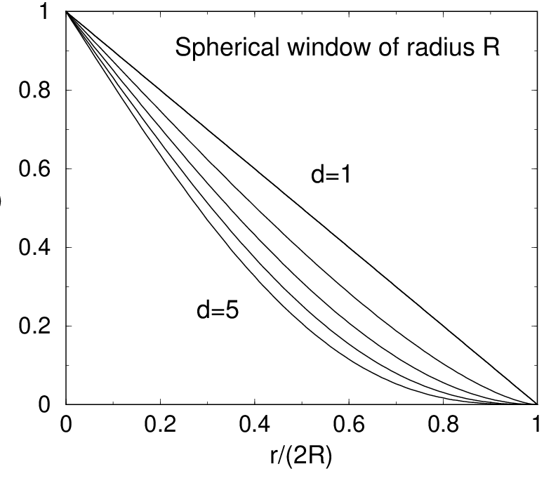
It has been shown that finding the point process that minimizes the number variance $\sigma^{2}(R)$ is equivalent to finding the ground state of a certain repulsive pair potential with compact support [18]. This problem is directly related to an outstanding problem in number theory involving generalized zeta functions and lattices [25]. Understanding such ground states can be facilitated by utilizing “duality” relations that link ground states in real space to those in Fourier space [26].

Here we obtain the appropriate generalization of (1) that corresponds to a determinantal point process in $\mathbb{R}^{d}$. First, we make the simple observation that the pair correlation function specified by (1) is related to the Fourier transform ${\tilde{\alpha}}(k;R)$ of the one-dimensional scaled intersection volume evaluated at $k=r$ and $R=\pi$, namely,

where ${\tilde{\alpha}}(k;R)$ is given by (26) for $d=1$. A natural generalization of this pair correlation function in $\mathbb{R}^{d}$ is to replace the one-dimensional Fourier transform in (38) with its $d$-dimensional counterpart (26) evaluated at $k=r$ and divided by $(2\pi)^{d}$, i.e.,

However, the value of $R$ in each dimension must be chosen so that such a pair correlation function corresponds to a determinantal point process in that dimension. In other words, if we take the positive semidefinite function $H({\bf r})$ to be given by the following radial function:

$R$ must be determined so that the conditions (28) and (30) are satisfied. Noting that the expansion of $|H(r)|^{2}$ for small $r$ to leading order is given by

and using the condition that $g_{2}(0)=0$ [cf. (30)] yields that

Now we must show that a pair correlation function (39) with $R=K$ satisfies the bounds of (30) and the bounds (28) on the spectral function ${\tilde{H}}(k)$. The square of the function $H(r)$, specified by (40), is clearly positive and achieves its maximum value of unity at the origin when $R=K$ and tends to zero in the limit $r\rightarrow\infty$, and hence the bounds of (30) are satisfied when $R=K$. Referring to relation (25) for the Fourier transform of the window indicator function, we see that the Fourier transform of (40) with $R=K$ is simply the indicator function

which automatically satisfies (28), where $w$ is specified by (16) and $K$ is given by (42).

In summary, we have demonstrated that there is a determinantal point process in $\mathbb{R}^{d}$ with $n$-particle densities given by (27) with the kernel

where $K$ is given by (42). We will call such a determinantal point process a “Fermi-sphere” point process because ${\tilde{H}}(k)$ corresponds to a spherical window indicator function in Fourier space and, as we will see, corresponds to the ground state of a fermionic system in which the Fermi sphere is completely filled (see Section 3). In particular, the pair correlation function of such a point process [33] is given by

Moreover, the corresponding structure factor, at unit number density, takes the form

where $\alpha(k;K)$ is the scaled intersection volume of two $d$-dimensional spheres of radius $K$ separated by a distance $k$, i.e., the function $\alpha(r;R)$, specified by (23), with the replacements $r\rightarrow k$ and $R\rightarrow K$. Relation (46) is easily obtained by taking the Fourier transform of the total correlation function defined by (31), where $H(r)$ is given by (44), and employing the definition (7) for the structure factor. It follows from the properties of $\alpha(k;K)$ in (46) that the structure factor $S(k)$ obeys the following bounds for all $k$:

and achieves its maximum value of unity for $k\geq 2K$. The corresponding cumulative coordination number is given by

Note that the first term in (48) is precisely the cumulative coordination number for a Poisson point process in $\mathbb{R}^{d}$ and that the second term is strictly negative for any $r>0$, which is a reflection of the short-range repulsive nature of the point process. We will show that for sufficiently large $r$, the dominant contribution to $Z(r)$ will be the Poissonian term $v(r)$. We will see it is the cumulative coordination number $Z(r)$, rather than the pair correlation function (contrary to conventional wisdom), that enables one to identify and quantify an effective “hard-core” diameter of the determinantal point processes.

It is instructive to examine the asymptotic behaviors of $g_{2}(r)$, $S(k)$, and $Z(r)$ for the Fermi-sphere point process. By virtue of the asymptotic properties of the Bessel function of arbitrary order, the small-$r$ and large-$r$ forms of the pair correlation function (45) are respectively given by

and

We see that $g_{2}(r)$ tends to zero quadratically in $r$ in the limit $r\rightarrow 0$, independent of the dimension. The coefficient of the quadratic term in (49) for positive $d$ attains it maximum value of $\pi^{2}/3=3.2898\ldots$ for $d=1$ and monotonically decreases with increasing dimension, asymptoting to $2\pi/e=2.3114\ldots$ in the limit $d\rightarrow\infty$. Moreover, $g_{2}(r)$ tends to unity for large pair distances with a decay rate that is controlled by the power law $1/r^{d+1}$ for any $d\geq 1$.

The latter result implies that the structure factor $S(k)$ tends to zero linearly in $k$ in the limit $k\rightarrow 0$. Using (23) and (46), it is easy to verify that as $k$ tends to zero at $\rho=1$

where $c(d)$ is a $d$-dependent positive constant given by (22). We see that at unit density, the point process in $\mathbb{R}^{d}$ for any $d$ is hyperuniform, and the structure factor $S(k)$ has a nonanalytic behavior at the origin given by $S(k)\sim|k|$ ($k\rightarrow 0$). The coefficient of the linear term in (51) for positive $d$ attains it minimum value of $1/(2\pi)=0.1591\ldots$ for $d=1$ and monotonically increases with increasing dimension such that it asymptotes to $e^{1/2}/(2\pi)=0.2624\ldots$ in the limit $d\rightarrow\infty$. In three dimensions, this unusual linear nonanalytic behavior of the structure factor at $k=0$ is a well-known property of bosons in their grounds states [10, 11, 12] and, more recently, has been shown to characterize maximally random jammed sphere packings [13].

In Fig. 3, we compare pair statistics in both real and Fourier space for $d=1$ and $d=3$ at unit density. We see that the amplitudes of the oscillations in $g_{2}(r)$ that are apparent for $d=1$ are significantly reduced in the corresponding three-dimensional pair correlation function. The smallest value of $r$ for which $g_{2}(r)$ attains its maximum value of unity, which we denote by $r_{0}$, is determined by the first positive zero of $J_{d/2}(Kr)$, which for sufficiently large $d$ is given by

Since $K$ increases with increasing $d$ and grows like $\sqrt{2\pi d/e}$ for large $d$, $r_{0}$ grows like the square root of $d$ for large $d$. Similarly, the smallest value of $k$ for which $S(k)$ attains its maximum value of unity grows with increasing $d$ and for large $d$ grows like $\sqrt{d}$.

The results immediately above enable us to obtain the following small-$r$ and large-$r$ forms of the cumulative coordination number:

and

It is straightforward to prove that the asymptotic result (54) is a rigorous lower bound on $Z(r)$ for all $r$ using the identity $\int_{0}^{\infty}dxJ_{d/2}^{2}(xK)/x=1/d$, the inequality $\int_{0}^{\infty}dxJ_{d/2}^{2}(xK)/x\geq\int_{0}^{r}dxJ_{d/2}^{2}(xK)/x$ for all positive $r$, and relation (48). Indeed, since $Z(r)$ is always nonnegative, we have the lower bounds

where the length scale

is the zero of $v_{1}(r)-1$. The length scale $D$ can be regarded as an upper bound on the effective hard-core diameter, which clearly grows with increasing dimension as vividly illustrated in Fig. 4, which compares the exact form of $Z(r)$ with the lower bound (4.1) for $d=3$ and $d=17$. For large $d$, the effective hard-core diameter is given by the asymptotic expression

which is seen to grow like the square root of $d$. This growth of the effective hard-core diameter with dimension is a conceptually important conclusion that runs counter to conventional understanding of corresponding fermionic systems, which identifies the inverse “Fermi” radius, i.e., $K^{-1}=1/[2\sqrt{\pi}\Gamma(1+1/d)^{1/d}]$ (a decreasing function of $d$) with an effective hard-core diameter. We elaborate on this point in Section 3.

The hyperuniformity of the point process implies that the number variance $\sigma^{2}(R)$ for a spherical window of radius $R$ must grow slower than $R^{d}$ (i.e., the window volume) for large $R$. However, the fact that the large-$r$ behavior of the pair correlation function is controlled by the power law $1/r^{d+1}$ means that $\sigma^{2}(R)$ must also grow faster than the surface area of the window or $R^{d-1}$. In particular, upon substitution of (45) into (13), an asymptotic analysis reveals that for large $R$

where $C(d)$ is a $d$-dimensional constant of order unity. We remark that a similar asymptotic scaling is expected to hold even when the observation window is non-spherical; a discussion of this point has been provided in [34]. We see that the number variance scaled by the window surface area, $\sigma^{2}(R)/R^{d-1}$, grows like $\ln(R)$, independent of the dimension. This unusual number variance growth law in three dimensions has also been recently seen in maximally random jammed sphere packings [13], which can be viewed as prototypical glasses because they are simultaneously perfectly rigid mechanically and maximally disordered. Note that the coefficient multiplying $\ln(R)$ in (60) decays to zero exponentially fast as $d\rightarrow\infty$, and, therefore, the surface-area term $R^{d-1}$ increasingly becomes the dominant one in the large-$d$ limit. This behavior should be contrasted with number variance for a Poisson point process, which grows like the window volume, i.e., $R^{d}$.

Figure 5 graphically depicts the Fermi-sphere point processes in one and two dimensions, which are generated using the algorithm of Hough et. al. [29]. Details and applications of this algorithm are reported by us elsewhere [14].

Here we consider a generalization of the Fermi-sphere point process in which $\tilde{H}(k)$ is an indicator function for concentric rings in reciprocal space; we denote the resulting determinantal process as the “Fermi-shells” point process. Without loss of generality, define $2m$ radii $k_{F}^{(j)}$, where $j\in\{1,2,\ldots,2m-1,2m\}$ and $m\in\mathbb{N}$, such that the region of $d$-dimensional space within the ball $B(0;k_{F}^{(1)})$ is empty, the annulus between $k_{F}^{(2)}$ and $k_{F}^{(1)}$ is filled, and so forth. We therefore have $m$ filled concentric rings in reciprocal space. Since the conditions for a determinantal point process are fulfilled for any indicator function in reciprocal space [35], the pair correlation function will still be given by (29). The calculation of $H(r)$ proceeds as follows:

which implies:

where $\mathfrak{F}$ denotes the Fourier transform to coordinate space.

It is important to note that the values of the various $k_{F}^{(j)}$ are not independent of each other and are constrained by the density (here set to unity) according to:

References

- [1] Dyson F J, Statistical Theory of the Energy Levels of Complex Systems. I, 1962 J. Math. Phys. 3 140
- [2] Dyson F J, Correlations between Eigenvalues of a Random Matrix, 1970 Comm. Math. Phys. 19 235
- [3] Mehta M L, 1967 Random Matrices (New York: Academic Press)
- [4] Montgomery H L, The pair correlation of zeros of the zeta function, in: 1973 Proc. Sympos. Pure Math. vol. 24 (Providence: AMS) pp. 181-193
- [5] Odlyzko A M, On the Distribution of Spacings Between Zeros of the Zeta Functions, 1987 Math. Comput. 48 273; Odlyzko A M, The -nd zero of the Riemann zeta function, in: van Frankenhuysen M and Lapidus M L, 2001 Dynamical, Spectral, and Arithmetic Zeta Functions (Providence: AMS) pp. 139-144
- [6] Rudnick Z and Sarnak P, Zeros of principal -functions and random matrix theory, 1996 Duke Math. J. 81 269
- [7] Katz N M and Sarnak P, Zeros of zeta functions and symmetry, 1999 Bull. Amer. Math. Soc. 36 1
- [8] Torquato S and Stillinger F H, Exactly solvable disordered sphere-packing model in arbitrary-dimensional Euclidean spaces, 2006 Phys. Rev. E 73 031106
- [9] Feynman R P, 1998 Statistical Mechanics (Boulder, CO: Westview Press)
- [10] Feynman R P, Atomic Theory of the Two-Fluid Model of Liquid Helium, 1954 Phys. Rev. 94 262
- [11] Feynman R P and Cohen M, Energy Spectrum of the Excitations in Liquid Helium, 1956 Phys. Rev. 102 1189
- [12] Reatto L and Chester G V, Phonons and the Properties of a Bose System, 1967 Phys. Rev. 155 88
- [13] Donev A, Stillinger F H and Torquato S, Unexpected Density Fluctuations in Jammed Disordered Sphere Packings, 2005 Phys. Rev. Lett. 95 090604
- [14] Scardicchio A, Zachary C E and Torquato S, 2008 submitted for publication
- [15] Stoyan D, Kendall W S and Mecke J, 1995 Stochastic Geometry and Its Applications (New York: Wiley)
- [16] Torquato S and Stillinger F H, New Conjectural Lower Bounds on the Optimal Density of Sphere Packings, 2006 Exp. Math. 15 307
- [17] Beck J, Irregularties of distribution I, 1987 Acta Mathemtica 159 1
- [18] Torquato S and Stillinger F H, Local density fluctuations, hyperuniformity, and order metrics, 2003 Phys. Rev. E 68 041113
- [19] Gabrielli A, Jancovici B, Joyce M, Lebowitz J L, Pietronero L and Labini F S, Generation of primordial cosmological perturbations from statistical mechanical models, 2003 Phys. Rev. D 67 043506
- [20] Gabrielli A and Torquato S, Voronoi and void statistics for superhomogeneous point processes, 2004 Phys. Rev. E 70 041105
- [21] Gabrielli A, Joyce M and Torquato S, Tilings of space and superhomogeneous point processes, 2008 Phys. Rev. E 77 031125
- [22] Torquato S and Stillinger F H, Controlling the Short-Range Order and Packing Densities of Many-Particle Systems, 2002 J. Phys. Chem. B 106 8354; ibid, 2002 106 11406
- [23] Scardicchio A, Stillinger F H and Torquato S, Estimates of the optimal density of sphere packings in high dimensions, 2008 J. Math. Phys. 49 043301
- [24] A sphere packing is a point process in which there is a minimal positive distance between any pair of points. According to Ref. [16], a disordered sphere packing in is one in which the pair correlation function decays to its long-range value of unity faster than for some .
- [25] Sarnak P and Strombergsson A, Minima of Epstein’s Zeta function and heights of flat tori, 2006 Inventiones Math. 165 115
- [26] Torquato S and Stillinger F H, New Duality Relations for Classical Ground States, 2008 Phys. Rev. Lett. 100 020602
- [27] Macchi O, The Coincidence Approach to Stochastic Point Processes, 1975 Adv. Appl. Probab. 7 83
- [28] Soshnikov A, Determinantal random point fields, 2000 Russian Mathematical Surveys 55 923
- [29] Hough J B, Krishnapur M, Peres Y and Virág B, Determinantal Processes and Independence, 2006 Probab. Surveys 3 206
- [30] Johansson K, Determinantal Processes with Number Variance Saturation, 2004 Comm. Math. Phys. 252 111
- [31] Burton R and Permantle R, Local Characteristics, Entropy and Limit Theorems for Spanning Trees and Domino Tilings Via Transfer-Impedances, 1993 Ann. Probab. 21 1329
- [32] Horn R A and Johnson C R, 2005 Matrix Analysis (Cambridge: Cambridge UP)
- [33] Note that for arbitrary density , the corresponding pair correaltion function is still given by (45) but with , which reduces to (42) for unit density.
- [34] Gioev D and Klich I, Entanglement Entropy of Fermions in Any Dimension and the Widom Conjecture, 2006 Phys. Rev. Lett. 96 100503
- [35] Costin O and Lebowitz J L, On the Construction of Particle Distributions with Specified Single and Pair Densities, 2004 J. Phys. Chem. B. 108 19614
- [36] Torquato S and Lu B, Chord-length distribution function for two-phase random media, 1993 Phys. Rev. E 47 2950
- [37] Torquato S, 2002 Random Heterogeneous Materials: Microstructure and Macroscopic Properties (New York: Springer-Verlag)
- [38] Torquato S, Lu B and Rubinstein J, Nearest-neighbor distribution functions in many-body systems, 1990 Phys. Rev. A 41 2059
- [39] McWeeny R, Some Recent Advances in Density Matrix Theory, 1960 Rev. Mod. Phys. 32 335
- [40] Slater J C, A Simplification of the Hartree-Fock Method, 1951 Phys. Rev. 81 385
- [41] Boyd R J and Coulson C A, The Fermi hole in atoms, 1974 J. Phys. B: Atom. Molec. Phys. 7 1805
- [42] Schwabl F, 2005 Advanced Quantum Mechanics 3rd ed. (Berlin: Springer-Verlag)
- [43] Minkowski H, Diskontinuitätsbereich für arithmetische Äquivalenz, 1905 J. reine angew. Math. 129 220
- [44] Tracy C and Widom H, Level-Spacing Distributions and the Airy Kernel, 1994 Commun. Math. Phys. 159 151
- [45] Rintoul M D, Torquato S and Tarjus G, Nearest-neighbor statistics in a one-dimensional random sequential adsorption process, 1996 Phys. Rev. E 53 450
- [46] Ginibre J, Statistical Ensembles of Complex, Quaternion, and Real Matrices, 1965 J. Math. Phys. 6 440
- [47] Torquato S and Lee S B, Computer simulations of nearest-neighbor distribution functions and related quantities for hard-sphere systems, 1990 Physica A 164 347
- [48] Lu B and Torquato S, Nearest-surface distribution functions for polydispersed particle systems, 1992 Phys. Rev. A 45 5530
- [49] Parisi G and Zamponi F, Amorphous packings of hard spheres for large space dimension, 2006 J. Stat. Mech.: Theory Exp. P03017
- [50] Zamponi F, Some recent theoretical results on amorphous packings of hard spheres, 2007 Phil. Mag. 87 485
- [51] Skoge M, Donev A, Stillinger F H and Torquato S, Packing hyperspheres in high-dimensional Euclidean spaces, 2006 Phys. Rev. E 74 041127
- [52] Torquato S, Uche O U and Stillinger F H, Random sequential addition of hard spheres in high Euclidean dimensions, 2006 Phys. Rev. E 74 061308