Commensurate quantum oscillations in coupled qubits

The universal gate for quantum computing consists of the single qubit and the entangling two qubit operations. Usually, electromagnetic oscillating fields such as microwave fields, laser pulses, and oscillating voltages have been used for single qubit operations. The atomic states of cavity-QED [1] and ion-trap [2] qubits are used as a natural basis of qubit states. In these cases the quantum Rabi-type oscillation can be analyzed in an approximation, called the rotating wave approximation (RWA). Similarly, the semi-classical Rabi-type oscillation of qubits of the artificial atomic states such as the superconducting charge qubit employed in the circuit-QED quantum computing [3] and the flux qubit [4] can also be analyzed in this approximation.

We study the coherent two-qubit oscillation driven by an oscillating field. The two-qubit oscillation enables the two-qubit gate for the quantum computing. Among the two-qubit gates the CNOT gate is the most basic two-qubit operation for the universal gate. [5] The CNOT gate operation was achieved in superconducting qubits with Ising-type interaction without driving oscillating field. [6] The oscillating-field-driven CNOT gate operation in superconducting qubits has recently been reported, but the fidelity is not so high due to the weak coupling strength between qubits. [7] In this study we propose a scheme for the CNOT gate operation between coupled qubits under an oscillating field for general Ising-type coupling strength. We discuss the CNOT gate operation for both the strong and weak coupling strength and show that the high fidelity of CNOT gate can be obtained even for a weak coupling.

The CNOT gate uses the discriminating operations corresponding to different states of control qubit. Depending on the control qubit states, the coupled-qubit state demonstrates a Rabi-type oscillation for the resonant oscillating field or non-resonant oscillation. During the $\pi$ rotation the target qubit state flips to the other qubit state for a control qubit state, while for the other control qubit state the target qubit state goes back to the original state before reaching the other state. Though the latter oscillation is far from the Rabi-type oscillation, the commensurate oscillations give rise to the CNOT gate operation. By using the commensurate mode oscillations we obtain high fidelity for the CNOT gate operation. We show that for a weak coupling a high performance CNOT gate can be achieved by tuning the parameters, while for a sufficiently strong coupling the maximum fidelity can be obtained regardless of the values of system parameters. The maximum fidelity for a weak coupling can be obtained for any fixed coupling strength and qubit energy gap by finely tuning the amplitude of oscillating field in an experimental setup. This scheme of using the commensurate oscillation is quite general, so it is applicable to the natural atomic qubits as well as the solid state qubits.

The Hamiltonian of a two level system (qubit $a$) driven by an oscillating field with frequency $\omega$ is given by

where

$\kappa$ is the external variable controlling the qubit energy levels, and $\sigma_{z,x}$ are the Pauli matrices. Here g is the coupling strength between the qubit and the oscillating field which is proportional to the amplitude of the oscillating field, $t_{\rm q}$ is the tunnelling amplitude between different (pseudo-) spin states, and $E^{a}(\kappa)=E^{a}_{\uparrow}(\kappa)-E^{a}_{\downarrow}(\kappa)$. The qubit energy gap $E^{a}(\kappa)$ can be controlled by $\kappa$, and for a particular value of $\kappa_{0}$ the qubit can be brought to the degeneracy point, $E^{a}_{\uparrow}(\kappa_{0})=E^{a}_{\downarrow}(\kappa_{0})\equiv E^{a}_{0}$.

At this point the dominant energy scale is the tunnelling energy $t^{a}_{q}$ and, if we introduce the coordinate transformation, $|0\rangle=(|\downarrow\rangle+|\uparrow\rangle)/\sqrt{2}$ and $|1\rangle=(|\downarrow\rangle-|\uparrow\rangle)/\sqrt{2}$, we have the Hamiltonian:

where ${\cal E}^{a}_{0(1)}=E^{a}_{0}\mp t^{a}_{q}$. Hence the resonant microwave with frequency $\omega=2t^{a}_{q}$ gives rise to the Rabi-type oscillation between the qubit states, $|0\rangle$ and $|1\rangle$.

When two qubits (qubits $a$ and $b$) are coupled, the Hamiltonian for coupled qubits in the basis of $\{|\downarrow\rangle,|\uparrow\rangle\}$ can be written as

with the Ising-type coupling strength $J$  [8, 9]

Here, $E_{ss^{\prime}}$ are the energy levels of coupled qubits, $E_{ss^{\prime}}(\kappa_{a},\kappa_{b})=E^{a}_{s}(\kappa_{a})+E^{b}_{s^{\prime}}(\kappa_{b})\pm J$ ($+$ for $s=s^{\prime}$, $-$ for $s=-s^{\prime}$), where $\kappa_{a}$ and $\kappa_{b}$ are the control variables for qubit $a$ and $b$, respectively. We here neglect the two-qubit tunneling term, $t^{ab}_{q}|s,s^{\prime}\rangle\langle-s,-s^{\prime}|$, because it is negligibly small for usual parameter regimes. This term gives rise to the XY-type interaction which enables the SWAP gate operation rather than the CNOT gate.

We can rewrite the Hamiltonian as

where $-s$ is the opposite spin of $s$, and

Afterward, we will omit $\kappa_{a},\kappa_{b}$ in $E_{ss^{\prime}}(\kappa_{a},\kappa_{b})$ for simplicity.

To perform a CNOT gate operation, the system parameters should be adjusted. We consider the situation that the external variables are adjusted in a way that (i) the energy gap $\Delta E=E_{ss^{\prime}}-E_{-ss^{\prime}}$ between different control qubit (qubit $a$) states is large and (ii) the target qubit (qubit $b$) is at a degeneracy point, $E_{\downarrow\downarrow}=E_{\downarrow\uparrow}$. This situation is usual for the CNOT gate operation of coupled qubits. [6, 8] In this case the tunneling process $t^{b}_{q}$ between different target qubit states takes a role, while $t^{a}_{q}$ between different control qubit states is negligible due to the large energy level difference $\Delta E$. Consequently, the two-qubit Hamiltonian $H$ becomes block-diagonal.

Figure 1(a) shows the energy levels $E_{ss^{\prime}}$ as a function of $\kappa_{b}$, where we choose $\kappa_{a}$ such that $|E_{ss^{\prime}}-E_{-ss^{\prime}}|\gg t^{a}_{q}$ and thus $t^{a}_{q}$ can be negligible. In the figure there are two degeneracy points; lower degeneracy point where $E_{\downarrow\downarrow}=E_{\downarrow\uparrow}$ and upper degeneracy point where $E_{\uparrow\downarrow}=E_{\uparrow\uparrow}$. By adjusting the variable $\kappa_{b}$, the coupled-qubit states can be brought to one of these degeneracy points. Here the distance between these degeneracy points is related to the coupling strength between two qubits. [6, 8]

Here we introduce a coordinate transformation,

with $\tan\theta_{s}=2t^{b}_{q}/|E_{s\downarrow}-E_{s\uparrow}|$ in order to couple the oscillating field with the off-diagonal elements of the qubit Hamiltonian. Then the Hamiltonian ${\cal H}=V^{-1}HV$ becomes

where

with $\alpha_{0}=\sin\theta_{\downarrow},~\beta_{0}=\cos\theta_{\downarrow},~\alpha_{1}=\sin\theta_{\uparrow}$ and $\beta_{1}=\cos\theta_{\uparrow}$. The two-qubit states $|\rho\rho^{\prime}\rangle$ are given as

where $s=\downarrow(\uparrow)$ for $\rho=0(1)$.

At the lower degeneracy point $E_{\downarrow\downarrow}=E_{\downarrow\uparrow}\equiv E_{0}$, we have the relations,

and

by using the relation of Eq. (5). Since the Hamiltonian ${\cal H}$ is block-diagonal, we have

where

Here, $\alpha_{1}g$ corresponds to the transition frequency between $|10\rangle$ and $|11\rangle$ states, while $\beta_{1}g$ term induces unnecessary complicate oscillations. In Fig. 1 the energy gaps are given as

where $\hbar\omega_{0}$ is the qubit energy gap, and $\hbar\omega_{1}$ depends on the qubit coupling strength through the relation

We here consider the case that the oscillating field is resonant with the energy gap $\omega_{0}$ between the states $|00\rangle$ and $|01\rangle$, i.e. $\omega=\omega_{0}$, at the degeneracy point $E_{\downarrow\downarrow}=E_{\downarrow\uparrow}$. Then this Hamiltonian describes the usual Rabi-type oscillation between the states $|00\rangle$ and $|01\rangle$ with the Rabi frequency $\Omega_{\rm R}\approx g/\hbar$, while the evolution of the states $|10\rangle$ and $|11\rangle$ is far from the Rabi oscillation, since the energy level difference is not resonant with the oscillating field frequency, $\omega_{1}\neq\omega$, for a finite coupling strength $J$.

We again introduce a rotating coordinate such as $\psi(t)=U(t)\phi(t)$, where

Accordingly, the Schrödinger equation ${\cal H}\psi(t)=i\hbar\frac{\partial}{\partial t}\psi(t)$ is written as $i\hbar\frac{\partial}{\partial t}\phi(t)=\tilde{{\cal H}}\phi(t)$ with $\tilde{{\cal H}}=U^{-1}(t){\cal H}U(t)-i\hbar U^{-1}(t)(dU(t)/dt)=\tilde{{\cal H}}_{0}\oplus\tilde{{\cal H}}_{1}$, where

and $\xi(t)=\omega_{0}t+2g\beta_{1}\sin\omega_{0}t/\omega_{0}$. From this Hamiltonian we can obtain the two-qubit oscillation numerically. Also the dynamics can be analyzed in the RWA.

The RWA assumes near resonance $\omega\approx\omega_{0}$ and weak coupling between a qubit and a oscillating field $g/\hbar\ll\omega_{0}$. [10] In the quantum Rabi oscillation for cavity-QED and ion-trap qubit, usually $g/\hbar\omega_{0}\approx 10^{-6}-10^{-7}$. For the usual superconducting qubits the coupling strength $g/\hbar\omega_{0}\sim$ O($10^{-1}$)  [3, 4] which is relatively strong, but we find that the RWA gives accurate results consistent with our numerical calculation.

The off-diagonal element of $\tilde{{\cal H}}_{0(1)}$ is written as

where $J_{n}(x)$ is the Bessel function of the first kind. In the usual RWA, the fast oscillating term $e^{2i\omega_{0}t}$ in $[\tilde{{\cal H}}_{0}]_{12}$ is neglected. Similarly we here neglect $e^{in\omega_{0}t}~(n\neq 0)$ in $[\tilde{{\cal H}}_{1}]_{12}$, resulting in

where $g^{\prime}=g\alpha_{1}\left[J_{0}\left(2g\beta_{1}/\hbar\omega_{0}\right)+J_{-2}\left(2g\beta_{1}/\hbar\omega_{0}\right)\right].$

Hence the Hamiltonian $\tilde{{\cal H}}^{\rm RWA}_{0}=(1/2)g\sigma_{x}=(g/\hbar)S_{x}$ describes the Rabi oscillation with the Rabi frequency $\Omega_{\rm R}=\Omega_{0}=g/\hbar,$ while the Hamiltonian $\tilde{{\cal H}}^{\rm RWA}_{1}$ shows a non-resonant oscillation with the oscillating frequency $\Omega_{1}=\sqrt{\left(\omega_{1}-\omega_{0}\right)^{2}+(g^{\prime}/\hbar)^{2}}.$ From the relation of Eq. (19) we see that the behavior of this non-resonant oscillation depends on the coupling strength $J$ as well as $\omega_{0}$ and $g$.

In Fig. 1(b) we show the resonant and non-resonant oscillations, when $\kappa_{b}$ is adjusted to the lower degeneracy point where $E_{\downarrow\downarrow}=E_{\downarrow\uparrow}$. Then a microwave with resonant frequency $\omega=\omega_{0}$ gives rise to the Rabi oscillation between two states $|00\rangle$ and $|01\rangle$, while the states $|10\rangle$ and $|11\rangle$ experience a non-resonant oscillation. The controlled-NOT gate operation requires that the target qubit flips for a specific state of control qubit such that $|00\rangle\rightarrow|01\rangle$ while $|10\rangle\rightarrow|10\rangle$. However, for example, at $\Omega t=\pi$ in Fig. 1(b) the states $|11\rangle$ and $|10\rangle$ also evolves during the transition from $|00\rangle$ to $|01\rangle$. Thus we cannot expect a good CNOT gate operation in this case.

Although, for $\omega_{1}$ different from the resonant value of $\omega=\omega_{0}$, the oscillation is not a Rabi oscillation, the oscillation period can be an even integer multiple of that of the resonant Rabi oscillation mode for a specific values for parameters $g$, $J$, and $\omega_{0}$ which correspond to the oscillating field amplitude, the coupling strength between qubits, and the qubit energy gap, respectively. The condition for this commensurate periods is given by

as we can see in Fig. 2. This condition determines the value of $g$ for given values of $(\omega_{0},J)$.

From Eq. (27) the value of $g$ for fidelity maxima can be expressed as

The argument of the Bessel function is written as $2g\beta_{1}/\hbar\omega_{0}=(2g/\hbar\omega_{0})4J/\sqrt{(\hbar\omega_{0})^{2}+16J^{2}}$. For $x\rightarrow 0$, the Bessel functions $J_{0}(x)$ and $J_{-2}(x)$ approach 1 and 0, respectively. Thus, for small $J$ and large $\omega_{0}$ the expression of $g$ in Eq. (28) can be approximated as

using Eq. (19). These expressions of Eqs. (28) and (29) provide the value for $g$ for the fidelity maxima with given values of $J$ and $\omega_{0}$.

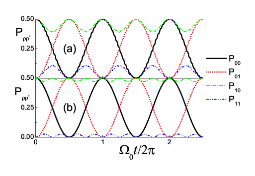
The scheme for CNOT gate operation in this study uses the non-Rabi oscillations for $|10\rangle$ and $|11\rangle$ states which are commensurate with the Rabi oscillation for $|00\rangle$ and $|01\rangle$ states. In Fig. 2 we display the numerical results obtained from the Hamiltonian in Eqs. (21) and (22), which show such commensurate mode oscillations. The initial state, $|\psi(0)\rangle=(|00\rangle+|10\rangle)/\sqrt{2}$, is driven by an oscillating field with the resonant frequency $\omega=\omega_{0}<\omega_{1}$.

In experimental situations usually the coupling $J$ and the qubit energy gap $\omega_{0}$ are set to be fixed. Thus the control of oscillating field amplitude $g$ with fixed $J$ and $\omega_{0}$ will be more desirable. For any given pair of $(\omega_{0},J)$ one can find a commensurate oscillation by finely tuning the value of $g$ according to Eq. (28). By varying $g$ with fixed $\omega_{0}$ and $J$, we were able to find a commensurate oscillation mode numerically; the oscillation period of the $|00\rangle$ and $|01\rangle$ states is twice of that of the $|10\rangle$ and $|11\rangle$ states [Fig. 2(a)], which corresponds to $n=1$ in Eq. (27). As $g$ decreases further, another commensurate mode with a shorter period appears in Fig. 2(b) ($n=2$). Actually we have found a series of commensurate modes as $g$ decreases. The values of $g$ obtained numerically coincide well with those from the RWA in Eq. (28) as shown in Table 1.

The CNOT gate operation is done when the occupation probability $P_{00}$ ($P_{01}$) is reversed perfectly from 0.5 (0) to 0 (0.5) at $\Omega t=$ (odd) $\pi$. At the same time, we can observe that the probabilities $P_{10}$ and $P_{11}$ recover their initial values 0.5 and 0, respectively. As a result, the CNOT operation is realized by using these commensurate oscillations.

Let us consider a concrete example for comprehensive understanding. For superconducting flux qubits, [4, 11] $g=mB$ is the coupling between the amplitude $B$ of the magnetic microwave field and the magnetic moment $m$, induced by the circulating current, of the qubit loop. In order to adjust the value of $g$, actually we need to vary the microwave amplitude $B$, because the qubit magnetic moment is fixed at a specified degeneracy point. The Rabi-type oscillation occurs between the transformed states $|0\rangle=(|\downarrow\rangle+|\uparrow\rangle)/\sqrt{2}$ and $|1\rangle=(|\downarrow\rangle-|\uparrow\rangle)/\sqrt{2}$. The states of qubits can be detected by shifting the magnetic pulse adiabatically [12]. Since these qubit states are the superposition of the clockwise and counterclockwise current states, $|\downarrow\rangle$ and $|\uparrow\rangle$, the averaged current of qubit states vanishes at the degeneracy point in Fig. 1(a). Thus, one can apply a finite dc magnetic pulse to shift the qubits slightly away from the degeneracy point to detect the qubit current states.

We now discuss the performance of CNOT gate operation. The fidelity for CNOT gate operation is given by $F(t)={\rm Tr}(M(t)M_{\rm CNOT})/4$,[7] where $M_{\rm CNOT}$ is the matrix for the perfect CNOT operation and $M(t)$ is the truth table amplitude at time $t$. In Fig. 3 we plot the fidelity $F$ by varying $g,~\omega_{0}$ or $J$ at $\Omega_{0}t=\pi$. In Fig. 3(a) the main and subsidiary maxima correspond to the CNOT operation in Fig. 2(a) and (b), respectively. As shown in Eq. (28) the fidelity maxima are determined by the three parameters, $g,~\omega_{0}$ or $J$. The series of maxima correspond to the different $n$ in Eq. (28). In the inset of Fig. 3(a) we also show the fidelity as a function of $\omega_{0}$.

An interesting behavior of fidelity maxima is shown in Fig. 3(b) as a function of $J$, where the fidelity approaches the maximum as the coupling strength $J$ increases. In the inset we show the oscillations for various parameters converge to 1, which implies that for sufficiently strong coupling maximum fidelity for the CNOT gate is achievable regardless of the values of other parameters. This is because, for a sufficiently strong coupling $J\gg\omega_{0}$, thus $\alpha_{1}=\sin\theta_{\uparrow}\approx 0$, the off-diagonal terms in Eq. (16) which induce the oscillation between two states with $\rho=1$ are vanishing and thus the occupation probabilities of the $|10\rangle$ and $|11\rangle$ states are not changed. As a result, the states $|10\rangle$ and $|11\rangle$ preserve their initial occupation probabilities, while the states $|00\rangle$ and $|01\rangle$ experience a Rabi-type oscillation. In this limit, the CNOT gate operation can be achieved with arbitrary parameter values.

In Fig. 4 we show the Rabi-type oscillation for strongly coupled qubits. While the $P_{00}$ ($P_{01}$) is reversed from 0.5 (0) to 0 (0.5) at $\Omega t=$ (odd) $\pi$, we can observe that the probabilities $P_{10}$ and $P_{11}$ remain their initial values 0.5 and 0, respectively. In this case the parameters need not satisfy the commensurate condition of Eq. (27) for the CNOT gate operation.

In fact, however, it is not so easy to obtain a sufficiently strong coupling between qubits in experiment. Instead, we can achieve a high fidelity of CNOT gate by choosing parameters satisfying Eq. (28). In real experiments we can control the amplitude of the oscillating field $g$, while the coupling $J$ and energy gap $\omega_{0}$ are fixed. In Table 1 we compare the numerical results for $g$ at the main fidelity maximum points ($n$=1) with those obtained from Eq. (28) in the RWA, which shows that two values fit well with each other. The approximate values are a little smaller than the numerical values and the small deviation tends to increase as $J$ increases and $\omega_{0}$ decreases. This can be understood from Eq. (29) where $g$ increases as $J$ increases and $\omega_{0}$ decreases. Hence for small $J$ and large $\omega_{0}$ the RWA and the numerical calculation coincide with each other, because the RWA works well in the regime $g/\hbar\ll\omega_{0}$. For the parameters far away from this regime the two-qubit oscillation deviates seriously from the Rabi oscillation and thus the CNOT gate operation cannot be performed, except the strong coupling limit discussed.

Though the value of fidelity at the main peak in Fig. 3 is close to the maximum value of 1, it has small deviation, $\delta F=1-F$. In Fig. 5 we plot the fidelity error $\delta F$ for various values of $(\omega_{0},J)$ at $\Omega_{0}t=\pi$. For large $\omega_{0}$ and small $J$ the fidelity error is vanishing, and the Rabi oscillation by the Hamiltonian ${\tilde{\cal H}}$ in Eqs. (21) and (22) is close to $\delta F\approx 10^{-4}$ for the fault-tolerant quantum computing. Hence for a weak coupling as well as a strong coupling we can achieve high performance CNOT gate operation.

The commensurate oscillations of resonant and non-resonant modes enable the high fidelity CNOT gate operation by finely tuning the oscillating field amplitude for any given values of qubit energy gap and coupling strength between qubits. While for a sufficiently strong coupling the CNOT gate can be achieved for any given parameter values, for a weak coupling a relation between the parameters should be satisfied for the fidelity maxima. For a sufficiently weak coupling compared to the qubit energy gap, $J/\hbar\omega_{0}\ll 1$, we have $\alpha_{1}\approx 1$ and $\beta_{1}\approx 0$, resulting in the expression for $g$ in Eq. (29). For $J/\hbar\omega_{0}\ll 1$, Eq. (29) immediately gives rise to the relation $g/J\ll 1$ and thus $g/\hbar\omega_{0}\ll 1$ after some manipulation. This means that for a weak coupling $J/\hbar\omega_{0}\ll 1$ the numerical results are well fit with the RWA as shown in Table 1, because the RWA is good for $g/\hbar\omega_{0}\ll 1$. As a result, the high performance CNOT gate operation can be achieved as shown in Fig. 5.

References

- [1] J. M. Raimond, M. Brune, and S. Haroche, Rev. Mod. Phys. 73, 565 (2001).
- [2] J. I. Cirac and P. Zoller, Phys. Rev. Lett. 74, 4091 (1995).
- [3] A. Blais et al., Phys. Rev. A 75, 032329 (2007); A. Wallraff, D. I. Schuster, A. Blais, L. Frunzio, R. S. Huang, J. Majer, S. Kumar, S. M. Girvin, and R. J. Schoelkopf, Nature 431, 162 (2004); G. S. Paraoanu, Phys. Rev. B 74, 140504(R) (2006).
- [4] I. Chiorescu, Y. Nakamura, C. J. P. M. Harmans, and J. E. Mooij, Science 299, 1869 (2003).
- [5] A. Barenco et al., Phys. Rev. A 52, 3457 (1995).
- [6] T. Yamamoto, Yu. A. Pashkin, O. Astafiev, Y. Nakamura, and J. S. Tsai, Nature 425, 941 (2003).
- [7] J. H. Plantenberg, P. C. de Groot, C. J. P. M. Harmans, and J. E. Mooij, Nature 447, 836 (2007).
- [8] M. D. Kim and J. Hong, Phys. Rev. B 70, 184525 (2004).
- [9] M. D. Kim, Phys. Rev. B 74, 184501 (2006).
- [10] E. T. Jaynes and F. W. Cummings, Proc. IEEE 51, 89 (1963).
- [11] J. E. Mooij, T. P. Orlando, L. Levitov, L. Tian, C. H. van der Wal, and S. Lloyd, Science 285, 1036 (1999); C. H. van der Wal, A. C. J. ter Haar, F. K. Wilhelm, R. N. Schouten, C. J. P. M. Harmans, T. P. Orlando, S. Lloyd, and J. E. Mooij, Science 290, 773 (2000); I. Chiorescu, P. Bertet, K. Semba, Y. Nakamura, C. J. P. M. Harmans, and J. E. Mooij, Nature 431, 159 (2004);
- [12] K. Kakuyanagi, T. Meno, S. Saito, H. Nakano, K. Semba, H. Takayanagi, F. Deppe, and A. Shnirman, Phys. Rev. Lett. 98, 047004 (2007); F. Deppe, M. Mariantoni, E. P. Menzel, S. Saito, K. Kakuyanagi, H. Tanaka, T. Meno, K. Semba, H. Takayanagi, and R. Gross, Phys. Rev. B 76, 214503 (2007).