The Concepts of “Age” and “Universality” in Cosmic Ray Showers
Abstract
The concept of “age” as a parameter for the description of the state of development of high energy showers in the atmosphere has been in use in cosmic ray studies for several decades. In this work we briefly discuss how this concept, originally introduced to describe the average behavior of electromagnetic cascades, can be fruitfully applied to describe individual showers generated by primary particles of different nature, including protons, nuclei and neutrinos. Showers with the same age share three different important properties: (i) their electron size has the same fractional rate of change with increasing depth, (ii) the bulk of the electrons and photons in the shower (excluding high energy particles) have energy spectra with shapes and relative normalization uniquely determined by the age parameter, (iii) the electrons and photons in the shower have also the same angular and lateral distributions sufficiently far from the shower axis. In this work we discuss how the properties associated with the shower age can be understood with simple arguments, and how the shapes of the electron and photon spectra and the relative normalization that correspond to a certain age can be calculated analytically.
pacs
96.50.S-, 96.50.sd, 13.85.TpI Introduction
The concept of the “age” of a shower has been in use in the cosmic ray community for more than half a century. The concept first emerged [1] in the study of the average longitudinal development of purely electromagnetic showers generated by photons or electrons. It was then also applied [2, 3] to the lateral distribution of electrons around the shower axis. Soon, it was also understood that it is possible and useful to assign an “age” also to individual showers, and that the concept is applicable also to showers generated by hadronic primary particles such as protons or nuclei.
Some recents works [4, 5, 6] have rediscussed the concept of of shower age for the showers generated by ultra high energy cosmic rays in the Earth’s atmosphere. Giller et al [4] and Nerling et al. [5] have studied with montecarlo methods the showers generated by high energy protons and nuclei in air, and have observed that the energy and angle distributions of the electrons (in this work with “electrons” we will refer to the sum of electrons and positrons) in the showers have shapes that to a good approximation are only determined by an age parameter defined as:
| (1) |
where is the depth in unit of radiation lengths and is the depth where the shower reaches its maximum size. The shower size is defined as the total number of charged particle integrated over all energy, and effectively coincides with the electron size. These results have been extended to the lateral distribution of electrons by Gora et al. [6]. This property of “universality” is obviously very important for the analysis and interpretation of high energy cosmic ray observations, and it is therefore desirable to have a deeper understanding of its origin and of its limitations.
In this work we want to review critically the concepts of shower “age” and “universality”. One of the main points we want to make is to argue that the definition of age of equation (1), while reasonably accurate in most cases, is in general not correct, and should be replaced by a better motivated and more accurate definition.
The essence of the concept of shower age can be understood observing that all showers at the maximum of their development are in an appropriate sense “similar” to each other (that is have the same “age”). This “similarity” is represented by the fact that in all showers at maximum the energy spectra of “most” electrons and photons have the same shape and the same relative normalization. These particles also have the same angular distributions (that are obviously strongly correlated with energy) and, for an equal density profile of the medium where the shower is propagating, also the same lateral distribution around the shower axis.
The idea that all showers at maximum, that is at the depth where the derivative of the shower size vanishes, are “similar” independently from the energy and nature of the primary particle, can be naturally be generalized, stating that all showers that have the same fractional rate of change with depth, that is the same “size slope” :
| (2) |
are also “similar”. This means that to each value of the correspond well determined shapes of the electron and photon spectra (again only valid for “most” particles) and a well determined relative normalization for the two populations. It is intuitive (and will be later verified by detailed calculations) that the energy spectra of electrons and photons become progressively softer as decreases going from positive (when the shower size grows) to negative (when the shower size decreases) values.
There is a one to one mapping between the values of the size slope and the values of the shower “age” . This mapping is encoded by a function that, in the notation introduced by Rossi and Greisen in their “classic” paper [1], is called . The general definition of the shower age is therefore:
| (3) |
where is the inverse function of . The function (that will be discussed in more detail in the following) is monotonically decreasing and has a single zero at , therefore according to equation (3) showers have age at maximum and age () before (after) maximum.
The definition of the age parameter (3) may seem at first sight (and in some sense actually is) arbitrary, since the size slope itself or any monotonic function of are also perfectly adequate to identify “similar” showers. The choice of the particular mapping of equation (3) is motivated by the fact that one can attach a direct physical meaning to the quantity . The shapes of the electron and photon spectra for above the critical energy (the electron critical energy is the average energy lost by an electron in a radiation length, and corresponds also to the electron energy for which radiative and collision losses are equal) and (with the primary particle energy) are well represented by a power law:
| (4) |
These power law behaviors stops when approaches (from above) the electron critical energy. For energies below the electron spectrum has a sharp cutoff, while the photon spectrum has a “knee” and takes the form . The precise shapes of the cutoff of the electron spectrum, of the knee of the photon spectrum (that is the transition from the form to the ) and the relative normalizations of the photon and electron spectra are all entirely determined by the age (or equivalently by the size slope ) and can be computed in detail.
The commonly used definitions of age in equation (1) always coincides with the general definition (3) at shower maximum and therefore, by construction, it is a reasonably good approximation for showers sufficiently close to maximum. The motivation for the more general definition may appear as only a formal question of “principle”. In fact in some circumstances the two definitions are significantly different, and the general definition gives the correct shower age. The definition (1) coincides with the correct one only for a particular shape of the shower longitudinal that is known as the “Greisen profile” [3]. In fact Greisen profile and the age definition (1) are intimately connected, and can be seen (with the mediation of the function ) as the integral and the derivative of each other. The Greisen profile (discussed below in section IV) describes accurately the average development of purely electromagnetic showers, but is only a rough approximation for the description of individual hadronic showers, and naturally fails completely in the description of neutrino–induced showers. The deviations of the definition (1) from the true age (3) are of the same order of the deviations of the profile of a shower from the Greisen profile that has the same .
The authors in [4, 5] have calculated with montecarlo methods the shape of the electron spectra in hadronic showers of different age. The parametrizations of their results are essentially identical to the shapes of the electron spectra in showers of the same age calculated several decades ago by Rossi and Greisen [1]. These modern works have therefore effectively only “rediscovered” with montecarlo methods what should be called the “Rossi–Greisen” spectra. We want to attract attention to this fact for three reasons. The first one is that it is obviously appropriate to give credit to the remarkable work of the pioneers. The second is that the works of [4, 5] do not include a discussion of photon spectra. The shapes of these spectra and their relative normalization with respect to the electron ones are also determined unambiguously by the shower age, and have been also computed explicitely by Rossi and Greisen. Finally the derivation of the spectral shapes obtained by Rossi and Greisen with analytic methods allows physical insights on the origin and limitations of the “universality” of the spectra, that are not easily deducible from a montecarlo calculation.
It should be stressed that the “universality” of properties for cascades of the same age has clearly limitations since it only applies to “most” but not all particles in the shower. For example, the “similarity” among showers at the maximum of their development, (that is at age ) does not imply that the showers simply differ by the absolute normalization of their electromagnetic component. Considering at first the case of purely electromagnetic cascades, at maximum the showers generated by a photon of initial energy contain (in essentially all cases) more high energy particles than the showers generated by photons of lower energy. These high energy particles are negligible in number and do not contribute significantly to the total size but in general carry an important fraction of the shower energy, they “feed” the shower development and influence its development. The showers generated by other types of primary particles have “cores” of different structure and particle content, and follow different development profiles.
This work is organized as follows: in the next two sections we review a very well known subject, discussing the average longitudinal evolution of purely electromagnetic showers first in “approximation A”, that is neglecting the electron ionization losses, and then in “approximation B”. The concept of age emerged naturally in these studies. In approximation B the shower equations have “elementary solutions” labeled by the parameter , these solutions correspond to the “universal spectra” of showers with age . The following section discusses the well known “Greisen profile” that describes the average longitudinal development of purely electromagnetic showers. Finally we discuss the evolution of individual hadronic showers, and give some conclusions.
II Electromagnetic Showers in Approximation A
The evolution of purely electromagnetic showers can be studied [1] using two sets of simplifying assumptions called “Approximation A” and “Approximation B”.
In approximation A the only processes considered for the shower development are pair production for photons, and bremsstrahlung for electrons. The differential cross sections for these processes are described by the asymptotic formulae valid at high energy. The electron energy losses due to collisions with electrons and nuclei of the medium are neglected.
The average longitudinal development of electromagnetic showers is described by the two functions and that give the differential energy spectra of electrons and photons at depth . In this work we are following the notation introduced by Rossi and Greisen in [1], however here we introduce different symbols. Rossi and Greisen indicate the differential (integral) electron spectrum as () and the photon spectrum as ; the subscript notation used here is more suitable to the extension of the formalism to hadronic showers where other particle types are present.
In approximation A the evolution of the electron and photon differential spectra is described by the two integro–differential equations:
| (5) | |||||
| (6) |
In the right hand side of equation (5) the first term describes the contribution, and the second one the () processes. In the right hand side of equation (6) the first term describes the contribution, and the second one photon absorption. The differential cross sections for bremsstrahlung and pair production , and the photon absorption cross section are given in appendix A.
II.1 Elementary solutions
In the system of equations (5) and (6) no energy scale is present. Accordingly these equations have a set of “elementary”, scale invariant solutions of form:
| (7) |
that are power laws in energy, and change exponentially with the depth . Inserting these solutions in the shower equations (5) and (6) one obtains a quadratic equation for that has the two solutions:
| (8) |
To each solution corresponds a photon/electron ratio:
| (9) |
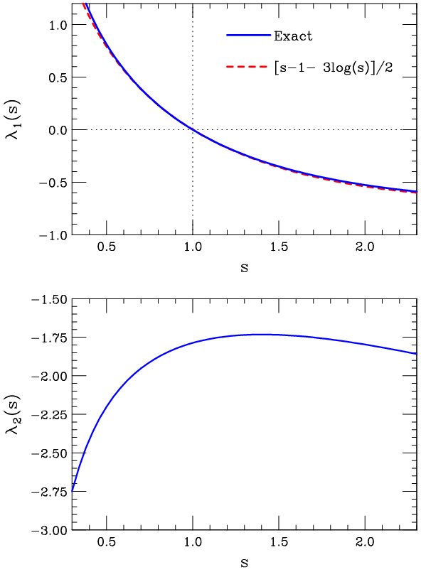
The auxiliary functions , and appearing in the definitions (8) and (9) are given explicitely in appendix A. The functions are shown in fig. 1, the function is shown in fig. 2.
Even if is already given by an explicit analytic expression in (8), it is very useful to follow Greisen [3] and introduce the simpler expression
| (10) |
that is a very good approximation for with deviations smaller than 2% in the interval . A comparison of the exact and approximate expressions for is shown in the top panel of fig. 1. The usefulness of this simpler functional form will be clear in the following.
The existence of two solutions for each value is physically simple to understand. If one starts at with populations of electrons that have power law form with the same slope, but arbitrary normalizations, the spectra mantain identical power law shapes at all , but change their relative and absolute normalization. The spectra reach first an asymptotic ratio with a scale , and then evolve exponentially mantaining a constant equilibrium ratio. The convergence to an asymptotic ratio is the fastest process since for all values.
As an explicit example, an initial power law, pure electron spectrum:
| (11) |
evolves in as:
| (12) |
The spectra remain power laws for all values. For one can set to zero, and the spectra evolve in as a simple exponential () with an asymptotic ratio that corresponds to the first solution in (9).
In summary, the solutions
| (13) |
is a sort of “attractor”, and any combinations of photon and electron spectra power laws spectra of the same slope “converge” to this solution.
The only independent solution corresponds to and is particularly important: The existence of this –independent solution:
| (14) |
and its energy dependence do not depend on the detailed form of the pair production and bremsstrahlung cross sections, and can be immediately understood observing that a power law spectrum of form contains equal amount of energy in each energy decade and that the bremsstrahlung and pair production processes that “mix” the electron and photon populations, conserve energy and are scale invariant. Only the value of the ratio that corresponds to this solution depends on the detailed form of the cross sections and is:
| (15) |
The fact that is positive (growing solution) for and negative (decreasing solution) for is also independent from the detailed form of the cross sections, and is a simple consequence of the fact that in a power law spectrum of form the energy contained in each decade increases with when and decreases when .
This very elementary discussion already illustrates how the –dependence of the shower development is intimately related to the shape of the energy spectra of the particles in the shower.
II.2 Showers generated by a primary or .
The evolution of the shower generated by a primary electron or photon of initial energy , in approximation A has been calculated by Rossi and Greisen [1]. Before describing these solutions explicitely we can observe that some important properties can be readily deduced with simple considerations. The differential spectra of electrons and photons in the solutions have the scaling form:
| (16) |
(the subscript runs over the 4 cases: , , and ). Correspondingly the integral spectra have the scaling form:
| (17) |
These scaling properties of the approximation A solutions are a simple consequence of the absence of quantities with the dimension of energy in the shower equations.
Energy conservation is reflected in the condition:
| (18) |
The solution of the shower equations for a monochromatic photon or electron [1] is very simple for the the Mellin transforms of and . The physically observable spectra can then be obtained inverting these transforms. The inversion can be easily performed numerically with a single path integration along a line in the complex plane, with exact results. Rossi and Greisen have also shown that it is possible to invert the trasform using a “saddle point approximation”, obtaining simple expressions for the spectra that are at the same time remarkably accurate and very instructive.
The saddle point approximation solution for the differential spectra (valid for large and ) can be written as:
| (19) |
with
| (20) |
For the integral spectra the saddle point approximation solution is:
| (21) |
Note that both the electron and photon integral spectra diverge for . For completeness a derivation of these well known results is sketched in appendix B, that also lists explicit expressions for the functions . An example of the differential spectra in approximation A is shown in fig. 3.
The saddle point solutions of the shower equations in approximation A exhibit several interesting properties:
- •
For a fixed value (less than unity) of the ratio (or ) the differential and integral spectra start at zero for , then grow with increasing , reaching a maximum at the value and then begin to decrease vanishing for . The exponential factor controls the evolution of the solution. Therefore in good approximation shower maximum corresponds to (and therefore to ). Using equation (20) one finds the well known result:
(22) On can therefore rewrite equation (20) in the form:
(23) - •
More in general, from the fact that the factor controls the dependence of the solution, it follows that to a good approximation one has:
(24) or
(25) - •
The quantity is related to the shape of the energy spectrum around , and has manifestly the meaning of the “local slope” of the spectrum at energy :
(26) In other words the spectrum around is well approximated as a power law . Globally the spectrum is not a simple power law and the “local slope” changes as a function of and . For a fixed depth the local slope grows monotonically with , as the spectrum becomes progressively steeper. For a fixed value of the spectrum also becomes steeper with increasing and as the local slope grows monotonically. The shape of the spectrum around energy takes the form when the spectrum for this energy reaches the maximum.
- •
Photons and electrons have spectra with very similar but not identical shapes, and accordingly the ratio changes slowly with energy. From the expressions for the functions (given in (79–82)) one finds:
(27) That is the “asymptotic ratio” for the elementary power law solution with slope . Note the remarkable fact that this result is independent from the nature of the particle ( or ) that initiates the shower.
- •
In fact the developments of showers initiated by a photon or an electron of the same energy are remarkably close to each other, demonstrating that the electron and photon population quickly tend to reach a sort of dynamic equilibrium feeding each other
In approximation A there is no natural way to associate a single age to a shower because the equations do not contain any meaningful energy scale (except the energy of the primary particle). Therefore for a given depth one can associate a different age to every ratio (or ) according to equation (20). The age describes at the same time the “stage” of the longitudinal evolution of spectrum (via equations (24) or (25)), and the shape of the spectrum near energy , that is well approximated by the power law . The age also controls the ratio around according to equation (27).
III Electromagnetic Showers in Approximation B
In approximation B the electron energy losses due to collisions are simply modeled as an energy independent loss per unit of radiation length. The quantity is the critical energy (in air MeV). Accordingly, a term is added to the right hand side of equation (5) that describes the electron evolution:
The new system of equations [() and (6)] does not have any more simple power law solutions of form (7). However, even in this case, one can introduce “elementary” solutions that have a constant shape in energy and evolve with with the simple behavior . Following Rossi and Greisen [1] the elementary solutions can be written in the form:
| (29) |
that contain two additional functions and . For large energy () the electron collision losses can be safely neglected, and the solutions coincide with the simple power law form of approximation A. This constraint tell us that the functions and that appear in (29) coincide with the functions discussed before and given in equations (8) and (9), and that for large the functions and asymptotically become unity:
| (30) |
Inserting expression (29) in the shower equations one obtains two pairs of integro-differential equations (see appendix C) for the functions and corresponding to the two solutions for . These equations can be solved numerically to obtain the functions and .
The physical meaning of the functions and is trasparent. If one injects power laws spectra of electrons and photons of form after a few lengths the spectra take asymptotically constant shapes given by:
| (31) |
(identical to (29) but selecting the first of the two possible solutions) and continue their evolve in as a simple exponential.
The qualitative features of this asymptotic solution are easy to understand. The electron spectrum is a nearly perfect power law for but has a cutoff for , when electrons are absorbed because of ionization losses. The photon spectrum changes from a power law for to the form for , reflecting the dependence of the bremsstrahlung cross section.
These physically intuitive properties are confirmed by the explicit calculation first performed by Rossi and Greisen, who have demonstrated [1] that the behavior of the functions and for is:
| (32) | |||||
| (33) |
The low energy behavior of the function implies that for the electron spectrum goes to a finite value. The energy integration of the electron spectrum therefore converges both for (if ) and for , and it becomes possible to talk about the total electron size. As expected the differential photon spectrum diverges for , and therefore the integral spectrum diverges logarithmically at the lower limit.
The total electron size for the phenomenologically most important solution (that corresponds to ) can be written as:
| (34) | |||||
The last equation defines the function . The physical significance of can be understood comparing equation (34) with the integral
The electron size obtained integrating over all the elementary solution (29) differs from the integration of the simple form in the interval ) by a factor . Rossi and Greisen have shown how to calculate exact values of the function for all integer values . For one has . A plot of the function is shown in fig. 9.
The functions and can be calculated with numerical methods, as discussed in Appendix C. For , it is also possible [1] (see again appendix C.1) to express the functions as power expansion in with easily calculable coefficients.
Figures 4 and 5 show (on a linear and log scale) the behavior of the electron spectrum plotted in the form for three values of the index . The integrated electron size is accounted for by particles in the energy range . Note that an important limitation of the treatment in approximation B is that the electron mass is neglected. Accordingly the electron spectra extends down to to unphysical energy values below the electron mass.
III.1 Solutions for monochromatic electron or photon
The solution of the shower equations in approximation B with the initial condition of a monochromatic electron or photon of energy cannot be given with an exact closed form expression. Rossi and Greisen suggest to approximate the solution with the expressions:
| (35) | |||||
| (36) |
with given by (20). These expressions combine the solution of the the shower equations in approximation A with the functions and introduced in section 2.2 as part of the “elementary solutions” to the shower equations. For the solution coincides with the one obtained in approximation A, while for the spectra have approximately the same shape of the “elementary solution” that corresponds to .
In approximation B, it in possible and natural to consider the value
| (37) |
as the age of the shower.
The total electron size of the shower obtained integrating over all energies is well approximated by the expression:
| (38) |
where we have used the fact that integration over energy is dominated by and the result (34). It can be easily seen, that the maximum of the size coincides with the condition , that implies and, solving equation (37):
| (39) |
Energy conservation in approximation B can be expressed with the equation:
| (40) |
The left–hand side of this equation is the energy contained in the shower particles at depth , while the second term in the right–hand side gives the energy dispersed in the medium by the electrons as ionization. Equation (40) also implies:
| (41) |
An example of the and spectra calculated in approximations A and B for a photon of initial energy eV at shower maximum is shown in fig. 6. The two solutions coincide for MeV, but deviate from each other at lower energy. The spectra in approximation B are strongly suppressed below the critical energy. The sum of the areas below the curves are proportional to the energy carried by each particle type. The curves of the approximation B solution enclose a smaller area because a part of the energy has been dispersed as ionization in the air (see equations (18) and (40)).
In approximation B showers generated by different primaries but having the same age according to the definition (37) have “essentially” equal spectra. This concept is illustrated in figure 7, that shows the electron spectra at shower maximum for showers generated by photons of different energy. The spectra are shown in two different representations. The first is of form ( versus ), in this case the area below the curve is proportional to the electron multiplicity. In the other representation the spectra are shown in the form ( versus ), in this case the area below the curve is proportional to the amount of energy contained in electrons. In showers of the same age most of the particles have coincident spectral shapes, however the distributions of the highest energy particles differ. High particles account for a significant fraction of the energy contained in the shower, and are the reason why the evolution with of a shower is not uniquely defined by the age, but depends also on the shower energy (or equivalently of the position where the age is achieved.
To summarize the results of this section: the explicit calculation of the average development of purely electromagnetic showers indicates that it is possible to define a shower age :
| (42) |
In showers of the same age the electrons and photons around and below the critical energy (that dominate the total number of particles in the shower) have the spectra of the same shape. The energy spectra differ at larger energy.
IV The Greisen profile
The average longitudinal development of a purely electromagnetic shower generated by a photon or electron of energy can be accurately described by a simple analytic expression introduced by Greisen [3]:
| (43) |
The “Greisen Profile” is essentially identical to the more complex expression given in (21). The derivation [3] of equation (43) is simple and instructive, and requires the intelligent “recombination” of some the the results obtained above.
The starting point of the derivation is the remark that the saddle point solution for the total electron size (38) indicates the approximate validity of the relation:
| (44) |
with the age given by (42). One can now substitute for the approximation given in (10) and rewrite equation (44) as:
| (45) |
The solution of this differential equation for the boundary condition is readily found as:
| (46) |
The normalization is fixed observing that the size at maximum for an electromagnetic shower can be obtained inserting the value in equation (38) with the result:
| (47) |
where we have used:
| (48) |
Substituting this results in (46) one obtains the final result (43). Expressions (38) and (43) “look” different from each other but are essentially coincident numerically.
A test of the accuracy of the Greisen profile solution can be performed verifying energy conservation using equation (41). This energy conservation condition is satisfied to better than 4.5% in the broad energy range from a few GeV to 1020 eV.
In summary, the Greisen profile (43) and the expression for the age in (1) (or 42) are equivalent to each other. The age definition (1) implies that the shower develops with the Greisen profile (45), viceversa the Greisen profile implies the simple functional dependence for the age of equation (1). The Greisen profile and the “Greisen age” (1) are (via the mapping ) the integral and the derivative of each other:
| (49) |
A recent paper by Schiel and Ralston [7] has complained that while the Greisen profile is shown and discussed many articles and textbooks, a full derivation is missing. The authors of [7] make an attempt to “reverse–engineer” the steps performed orginally performed by Greisen to obtain this result, and arrive at the surprising and erroneous conclusion that the Greisen profile was “likely motivated by early numerical work in a time predating high–speed computer”. These comments miss the essential point that the Greisen profile is the result of the exact integration of a well defined (albeit product of some approximations) differential equation.
The work [7] contains also a serious error when it argues that performing the derivative of the Greisen profile with respect to the critical energy and setting the value , one obtains the electron differential spectrum at the energy for a shower of primary energy at the depth . This error originates in a confusion between approximation A and approximation B for the shower equations, or perhaps more accurately in using the crude assumption to consider approximation B as nothing else than the introduction of a “sharp” cutoff for the electron spectra of approximation A for .
In fact performing the “trick” of the derivative with respect to in the energy interval . yield an interesting result that is proportional (but not equal) to the electron differential spectrum:
| (50) |
(with according to equation (42)). This result can be obtained comparing equations (21) and (38). When aproaches the interpretation of the derivative in (50) ceases to be valid, and the electron spectrum takes the “universal” (age dependent) shape with appropriate normalization.
This last exercise is however instructive in the sense that it illustrates an important point. The age determines the shape of the energy spectra of the “bulk” of the electrons and photons in the shower, but the distribution of the high energy particles depends on additional parameters. For the average development of an electromagnetic shower the ony additional parameter is the primary particle energy (or equivalently the position of maximum . The high energy particle content is crucial for the overall development of the shower. The Greisen profile implies that at each level the shower contains a spectrum of high energy particles that is consistent with the shape of the development. This high energy particle content is not determined by the shower age, but (for each age) depends also on the primary particle energy . The high energy () electron spectrum can be “extracted” from the shower profile via equation (50).
V Universality
As discussed in the introduction, the recent works of Giller et al. [4] and Nerling et al. [5] have shown that for the same shower age (using the definition of equation (1)), individual showers of hadronic primaries have electron spectra of the same shape. This result is clearly an important generalization of the result obtained in the previous section that the average development of purely electromagnetic showers.
In the following we want to:
- 1.
- 2.
- 3.
Show that also the shape of the photon energy distribution and its normalization relative to the spectrum of electrons in the shower are “universal” and determined by the shower age.
As an example of the numerical coincidence of the Rossi–Greisen spectra of equation (29) with the shape of the electron spectra calculated with montecarlo methods for the same value of the parameter , in fig. 8 we compare the function for the value with the equivalent quantity (that is ) from the fit to the electron spectra at shower maximum obtained by Nerling et al. [5]. The two functions are nearly coincident, and agreement of comparable quality is obtained for all age values in the phenomenologically most important range (for more discussion see appendix D). It is also interesting to note that the parametrization of [5] for the electron spectrum has the form:
| (51) |
that has manifestly the same asymptotic behavior as the Rossi–Greisen shape at both low and high energy: constant for , and for .
The fact that the energy spectra calculated of individual hadronic showers coincide with remarkable accuracy with spectral shapes calculated for the average development of purely electromagnetic showers may appear at first sight surprising, but it is of course not a simple numerical coincidence, and has in fact a natural explanation.
The first simple point is that in all shower types (electromagnetic, hadronic and also neutino induced) the total number of charged particles is essentially always (with the exception of very early and very late stages of development) dominated by electrons with energy around the critical energy . In hadronic shower this happens because in each hadronic interaction a large fraction of the energy is transfered to photons via the production and decay of and mesons, these photons then generate the electromagnetic part of the shower that accounts for a growing fraction of the shower energy, and for most of the particles in the shower.
The “universality” of the spectra in different showers of the same age, can then be immediately relating the “age” with the size slope according to equation (3), and observing that the arguments outlined in the previous sections can be generalized to conclude that that the size slope must be associated to a well defined shape for the “bulk” of the electrons and photons and to a well defined relative normalization between the two populations.
For example, at shower maximum, when the shower size is “stationary” (), the photon and electron spectra must have spectral shapes and relative normalization that insure this stationarity of the shower size. A stable solution for this problem has been found in the previous section and is:
| (52) |
To demonstrate formally that this in fact the general structure of the electron and photon spectra at shower maximum is in fact not trivial, however this is a very natural conclusion, observing how the result (52) emerge as the spectra at shower maximum for the average devolopment of the shower generated by both electrons or photons of arbitrary energy.
Similarly, for each size slope the quantity can be be identified with the parameters that labels the shape of the electron and photon spectra according to equation (31). The argument that we have outlined to relate the age and the electron and photon energy spectra is independent from the nature of the primary particle, from its energy, and from the value of the depth where the shower is measured.
The argument however does not allow to estimate the age from a closed form relation of type such as equation (1). The fact that this is impossible can be easily illustrated with the example of the shower generated by a neutrino. In this case the of the shower can of course be arbitrary large, and therefore for example the definition (1) returns for the entire shower development , that is of course meaningless, while it is physically transparent that the age concept mantain its validity and applicability, and the general definition (3) has no difficulty in dealing with neutrino induced showers.
One may think that the neutrino example described above is “artificial” and that the problem that emerged can be “solved” for example shifting the origin of the depth measurement to the neutrino interaction point. However this point is in most cases unobservable, and this shifting procedure is operationally not well defined (and would open the problem of performing a similar shift of the origin of the measurements also for hadrons and photon primaries).
Another way of to see the problem for a closed form expression of the age of form is that such a definition implies via equation (44) the entire longitudinal profile of the shower. For example, as discussed before, the expression (1) implies that the shower develops with the Greisen profile (45) (and viceversa). In general the longitudinal development of cosmic rays showers cannot be described accurately with the form (45), and this failure implies limitations for the approximate definition (1).
V.1 The “Gaisser Hillas” longitudinal profile
The observations of longitudinal profile of high energy showers obtained with the detection of fluorescence light, using the technique pioneered by the Fly’s Eye detector, and currently in use by the HiRes and Auger collaboration, are commonly fitted using a 4–parameters expression known as the “Gaisser–Hillas” profile: [8]:
| (53) |
The maximum of this function is at , where the size is equal to , while and modify the shape. The Gaisser–Hillas profile (53) implies the shower age:
| (54) |
where is the inverse function. of . For completeness we note that the inverse of the function can has the explicit form: . To study the age near shower maximum, one expand in a power series around the position of the maximum, using as expansion parameter the quantity :
| (55) |
The first terms in the series expansion are:
| (56) |
For comparison, the age near shower maximum for the Greisen profile (45) can be written as a power expansion in the quantity :
| (57) |
with the result:
| (58) | |||||
A comparison of the expansions (56) and (58) shows explicitely how precisely expression (58) maps the true age of a shower.
VI Conclusions and Outlook
The concept of the shower age can be very useful for the analysis of high energy cosmic ray data. The essence of the idea is very simple and can be summarized in a nutshell saying that the –slope and the –slope of a shower are connected to each other by a one to one mapping. The –slope (or size slope) is the fractional rate of change of the shower size with increasing depth (). The –slope (or energy slope) is the integral slope of the (power law) energy spectra of photons or electrons above the critical energy. The mapping between and is given by . The spectra of photons and electrons have a more complex shape around and below that is also determined by (or ), and have a relative normalization also determined by (or ). It is remarkable that the electron and photon spectra that correspond to different (or ) have been calculated accurately with analytic methods by the pioneers Rossi and Greisen many decades ago.
These properties of “universality” extend to the angular and lateral distributions of electrons and photons. This crucially important subject is not discussed here (see appendix E for some remarks).
The definition of age discussed here is independent from the shape of the longitudinal development of a shower, and is therefore more general and accurate that the commonly used definition that is correct only when the shower development is described by the “Greisen profile”. The average shape (and the fluctuations around this average) of the longitudinal development of high energy cosmic ray showers is determined by the nature of the primary particles and by the properties of hadronic interactions. The observation of these shape is a very important subject for future experimental studies.
A definition of age that depends only on the derivative of the shower size can be applied also to neutrino–induced showers, and more generally is expected to remain valid for the description of all shower where the size is dominated by electrons. This includes showers generated by exotic primaries, or the presence of unexpected physics (or unexpected fluctuations) in the development of the showers by primary particles of known nature. The search for events that have unusual longitudinal developments, such as multiple maxima is an interesting direction of research. It is likely (and at least the best possible a priori assumption) that the spectra of the electromagnetic component around and below the critical energy will, also in these cases, be controled by the shower age.
These ideas can be useful in the analysis of high energy cosmic ray observations in several ways. As examples: (i) the knowledge of the variations of the electron energy spectrum during the evolution of a shower can be used to obtain a better reconstruction of the longitudinal profile of the shower in observations that use fluorescence and/or Cherenkov light detectors (see [9] for more discussion); (ii) the reconstruction of the shower age from the lateral distribution of its electromagnetic component can in principle help in the reconstruction of the energy in surface array measurements; (iii) in case of hybrid measurements of the showers, the redundant measurement of the age (from the size longitudinal development and the lateral distribution of the electromagnetic component at the ground) can allow to disentangle a muon component, allowing composition measurements, or test of hadronic interaction models (see [10] for more discussion).
It should finally be stressed that the “universality” in the electromagnetic component of high energy showers, is clearly an important analysis tool, but gives only a partial information about the shower. Other information is contained in the shower muon component, moreover the shower core, that is essentially undetected in large area shower arrays, in most cases also contains a significant amount of energy. The energy contained in the core must be “infered” from the information obtained at large distances from the shower axis, introducing unavoidably some model dependence in the energy reconstruction.
Acknowledgments.
It is a pleasure to acknowledge fruitful discussions
with Ralph Engel, Maurizio Lusignoli and Silvia Vernetto.
Appendix A Cross sections for fundamental processes
In this appendix we list the expressions of the differential cross sections for the bremsstrahlung and pair production, the fundamental processes that control the development of electromagnetic showers. It is convenient to measure the column density in units of radiation length (with the notation ). The radiation length in air [12] is approximately 36.66 (g cm2)-1.
The probability per unit of radiation length that an electron of energy emits a photon of energy has the asymptotic form:
| (59) |
For the pair production process , the energy distribution of the final state electron is:
| (60) |
with . Integrating over all values one obtains the pair production probability per radiation length:
| (61) |
In the previous equations depends on the atomic number of the medium:
| (62) |
For air one has .
Important momenta of the functions and are:
| (63) | |||||
| (64) | |||||
| (65) |
In equation (63) is the digamma function and is the Euler gamma constant .
Appendix B Shower equations in approximation A
In this section we sketch a derivation of the solutions of the shower equations in approximation A for the initial condition of a monochromatic electron or photon.
The first step is to introduce the Mellin transforms and of the electron and photon spectra and . In general the Mellin transform of the function is defined as:
| (66) |
with a complex parameter. The Mellin transform converges in a strip bounded by two straight lines parallel to the imaginary axis (). The inverse transformation is:
| (67) |
where the integration path runs parallel to the imaginary axis within the strip of convergence of .
Applying the operator:
to the shower equations (5) and(6) one obtains a system of two linear differential equations for and :
| (68) | |||||
| (69) |
The general solution of this system can be easily obtained as a linear combinations of the exponential functions and .
The shower generated by an electron of energy at depth corresponds to the initial condition:
| (70) |
or:
| (71) |
while the shower generated by an initial photon of energy corresponds to the initial conditions:
| (72) |
or:
| (73) |
Using these boundary conditions one finds the solutions:
| (74) |
and
| (75) |
The functions can be obtained inverting the Mellin transformation using (67), or more explicitely:
| (76) |
(with the subscript than runs over the 4 cases: (), (), () and ()). This integral cannot be done exactly analytically, however with modern tools it is trivial to obtain the numerical result with any desired level of accuracy. In fact the integrand function is well defined (and available in computer libraries) for all complex values . The imaginary part of the integral vanishes while the real part gives the physically observable spectra.
Rossi and Greisen have also shown that using the “saddle point” approximation it is possible to obtain simple analytic expressions that are a very good approximation of the exact results for not too small, and that remain very instructive and useful. The basic idea behind the saddle point approximation is that the integrand in (76) is an analytic function in the variable . For any analytic function one has:
This implies that if the function has a minimum for a real value when runs along the real axis, the function will then have a maximum at the same point along a path that is at right angle with respect to the real axis. The integral is then dominated by the value of the function near the maximum, and can be performed analytically approximating the integrand with a Gaussian function, and using the well known result that if is a quadratic form:
with coefficient , one has:
| (77) |
(where is the point where the quadratic form is minimum, and the integrand is therefore maximum).
One can now apply this idea to the integral (76). For not too small, one can neglect the term proportional to in the expressions for the Mellin transforms given in equations (74) and (75) and rewrite the integrand of the inverse transform as:
| (78) |
where the functions are:
| (79) | |||||
| (80) | |||||
| (81) | |||||
| (82) |
In equation (78) the integrand of the inverse Mellin transform has been written as the product of a function that changes rapidly with (in square parenthesis) and a function that is considered as slowly varying. The part of the function that is rapidly varying with has a minimum along the real axis for the value determined by the implicit equation:
| (83) |
or equivalently:
| (84) |
This equation has an explicit solution if one substitutes for the Greisen analytic approximation given in (10). The solution is:
| (85) |
One can now complete the calculation at the saddle point approximating the integrand as a gaussian function and using equation (77) with with the result:
| (86) |
The integral distributions can be calculated noting that for not too small the integration is dominated by close to . Neglecting the slow variation of with one finds:
| (87) |
An alternative method to obtain equation (87) is to observe that if is the integral of the function for , then the Mellin transform is given by:
| (88) |
and performing the inversion with the the saddle point approximation.
For completeness we note that Rossi and Greisen suggest some slightly more complex forms for the saddle point solutions in place of equations (86) and (87) for a better approximation with the exact solution. The idea is to make a better choice for the “fast varying” part of the Mellin transform. This can be done introducing the quantity and rewriting the decomposition (78) as:
| (89) |
The esponent is chosen “ad–hoc” for better quantitative results. Rossi and Greisen [1] suggest the values:
| (90) | |||||
| (91) |
The part of the function that is considered as varying rapidly with is indicated in square parenthesis in (89) and has a minimum along the real axis for the value determined by the implicit equation:
| (92) |
that can be solved explicitely if one substitutes with the Greisen analytic approximation. The solution is:
| (93) |
One can proceed with the saddle point solution, noting that for the Gaussian approximation of the rapidly varying function the parameter is now given by: . The differential spectra can then be written as:
| (94) |
Similarly a more complex expression can be written to improve on equation (87) for the integral spectra. For large and large one can neglect the terms and the more complex expressions for the differential and integral spectra coincide with the simpler results (86) and (87).
Appendix C Elementary solutions in approximation B
The form of the solution for the shower equation in approximation B is given in equation (29). Inserting this expression in the shower equations one obtains two integro-differential equations for the functions and :
| (95) | |||||
and
| (96) |
It is possible to eliminate the function in (95), obtaining an equation for :
| (97) | |||||
The two solutions for are obtained substituting in (97) the two solutions for given in (8). Note that equation (96) is a simple integral, therefore from the knowledge of the electron energy spectrum, that is the functions , it is trivial to obtain numerically the corresponding photon spectrum, while it is not entirely trivial to solve numerically equation (97) for .
C.1 Power Expansion for the functions and
A useful result obtained by Rossi and Greisen is the demonstration that the functions and can be expressed as a power series in :
| (98) | |||||
| (99) |
with easily calculable coefficients. In fact, inserting these power series forms in equations (97) and (96) one obtains simple recursive relations for the coefficients:
| (100) |
| (101) |
where the function is:
| (102) |
and the functions , and are listed in appendix A. Clearly a power series in solution cannot be used for close or below unity (that is for close or below the critical energy ), however this expansion allows to test in its range of validity solutions obtained with different methods.
Appendix D Analytic and Montecarlo solutions
The calculation of the spectra of electrons and photons in shower of the same age obtained by Rossi and Greisen in [1] and discussed in this paper has the limitations that are intrinsic to the realistic but simplified theoretical framework (approximation B) that has been used. This framework introduces several simplifications: the cross sections for bremsstrahlung and pair production have always the asymptotic form that is strictly speaking only valid at very high energy, the electron collision losses are treated as a simple energy independent constant, and Compton scattering is entirely neglected. Also in approximation B the electron mass is neglected and the electron spectrum extends down to zero energy. A montecarlo calculation of the spectral shapes can of course avoid all these limitations and is in principle more accurate, even if it has its own limitations and difficulties
A comparison of the Rossi–Greisen shapes with the numerical results of [4, 5], shows remarkable agreement but also some small differences, that could be interesting to explore in more detail. As an illustration, normalizing the high energy spectra to , the quantity
| (103) |
is given by the function for the Rossi–Greisen calculation. The numerical integration of the Nerling et al parametrization [5] gives results that differ by 5–10% (at shower maximum the difference is 4.5%). A comparison of the results is shown in fig. 9.
As an additional test we have calculated the first coefficient in the development:
| (104) |
For the Nerling parametrization (51) the first coefficient is , while for the Rossi–Greisen solution the coefficient is given by (100). A comparison of the two estimate is shown in fig. 10.
The origin of the (small) differences between the analytic and montecarlo solutions merits further studies. A possible explanation is a more precise description of the physics of the electromagnetic interactions in the montecarlo calculation.
Appendix E Lateral Distribution
It is intuitive that in showers of the same age “most” electrons and photons have not only the same energy distributions but also the same angular distributions and, for the same density profile of the medium where the showers are propagating, also essentially equal lateral distributions around the shower axis.
The problem of calculating the electron lateral distribution has attracted considerable in the past. Nishimura and Kamata [2] solved numerically the 3–dimensional shower equations in approximation B to obtain the (energy integrated) lateral distribution of electrons propagating in a medium of constant density. Their result were fitted by Greisen [3] with the approximate form:
| (105) |
with is the Moliere radius and is a normalization factor. After these works several other authors have given different parametrizations of the lateral distribution as a function of an age parameter (see for example Hillas in [11].
In the view of this author it is in fact not possible to have a single parametrization for lateral distribution, because it is essential to consider the properties of the detector that measure the shower at the ground. For example the results of Nishimura and Kamata refer to the total number of electrons integrated down to zero energy, however in most cases the detectors of shower arrays do not sample the electron number but an energy deposition, and in any case it is always needed to take into account some contribution from photons in the shower. Therefore one needs to combine appropriately the electron and photon contributions with the detector response. An additional complications is of course that for hadronic primaries one has to disentangle the the electromagnetic and muon components of the shower.
References
- [1] Bruno Rossi & Kenneth Greisen, Rev. Mod. Phys. 13, 240 (1941).
- [2] J. Nishimura and K. Kamata Progr. Theor. Phys. 6, 93 (1958).
- [3] K. Greisen, Ann. Rev. Nucl. Part. Sci. 10, 63 (1960).
- [4] M. Giller,, G. Wieczorek, A. Kacperczyk and W. Tkaczyk J. Phys. G: Nucl. Part. Phys. 30 97 (2004).
- [5] F. Nerling, J. Blumer, R. Engel and M. Risse, Astropart. Phys. 24, 421 (2006).
- [6] D. Gora et al., Astropart. Phys. 24, 484 (2006) [arXiv:astro-ph/0505371].
- [7] R. W. Schiel and J. P. Ralston, Phys. Rev. D 75, 016005 (2007) [arXiv:hep-ph/0607248].
- [8] T. Gaisser and A.M. Hillas, Proc. 15th ICRC, Plovdiv, 8 353 (1977).Z
- [9] M. Unger, B. R. Dawson, R. Engel, F. Schussler and R. Ulrich, arXiv:0801.4309 [astro-ph].
- [10] R. Engel (Auger Collaboration), arXiv:0706.1921 [astro-ph].
- [11] A. M. Hillas, J. Phys. G 8, 1461 (1982).
- [12] W. M. Yao et al. [Particle Data Group], J. Phys. G 33, 1 (2006).