Unknotting Sequences for Torus Knots
Abstract.
The unknotting number of a knot is bounded from below by its slice genus. It is a well-known fact that the genera and unknotting numbers of torus knots coincide. In this note we characterize quasipositive knots for which the genus bound is sharp: the slice genus of a quasipositive knot equals its unknotting number, if and only if the given knot appears in an unknotting sequence of a torus knot.
1. Introduction
The unknotting number is a classical measure of complexity for knots. It is defined as the minimal number of crossing changes needed to transform a given knot into the trivial knot [14]. An estimate of the unknotting number is usually difficult, even for special classes of knots such as torus knots. It is the content of the Milnor conjecture, proved by Kronheimer and Mrowka [7], that the unknotting number of torus knots coincides with another classical invariant of knots, the slice genus. The slice genus of a knot is the minimal genus among all surfaces smoothly embedded in the 4-ball with boundary . In general, the slice genus of a knot provides a lower bound for its unknotting number :
Loosly speaking, this genus estimate tends to be good for quasipositive knots. A knot is quasipositive, if there exists a quasipositive braid, i.e. a braid which is a finite product of conjugates of the positive standard braid generators , whose closure is . Quasipositive knots, or rather links, are precisely the knots or links that arise from intersections of complex plane curves with the unit -sphere in ([3], [11]). In this note we characterize quasipositive knots for which the genus estimate is sharp. For this purpose we introduce the following terminology: an unknotting sequence for a knot is a finite sequence of knots
such that:
- (1)
, (in particular, is the trivial knot),
- (2)
two succeeding knots of the sequence are related by one crossing change.
We say that a knot can be unknotted via a knot , if is contained in an unknotting sequence for . It should be mentioned that unknotting sequences are highly non-unique: every knot of unknotting number at least two can be unknotted via infinitely many different knots [2].
Theorem 1.
Let be a quasipositive knot. Then the equality holds, if and only if there exists a torus knot that can be unknotted via .
Examples.
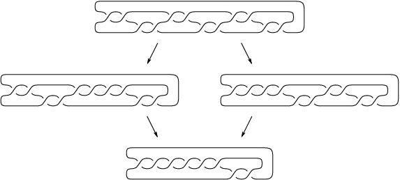
The three knots , and (in Rolfsen’s notation [10]) are positive, hence quasipositive by Nakamura and Rudolph ([8], [13]). Moreover, they all satisfy the equality . According to Theorem 1, they are to be contained in some unknotting sequences for torus knots. Actually, they are all contained in the following two unknotting sequences for the torus knot :
, , , unknot,
, , , unknot.
These two sequences are depicted in Figure 1 (the first one on the left; the second one on the right). The knot diagram at the top of the figure is a non-minimal two-bridge diagram for the torus knot .
Likewise, every positive twist knot with an odd number of crossings is contained in an unknotting sequence of the torus knot . In contrast, the slice quasipositive knot is not contained in any unknotting sequence of a torus knot, since .
Remark.
Theorem 1 stays true if we replace the slice genus by any invariant that coincides with on quasipositive knots, for example the concordance invariants or coming from knot Khovanov homology and Floer homology, respectively (see [5] for a comparison of these two invariants).
The assumption of Theorem 1 that be quasipositive is essential, as we can see by looking at the figure-8 knot with : if the figure-8 knot were contained in the unknotting sequence of a torus knot, then its unknotting number would have to coincide with its Rasmussen invariant . Indeed, the concordance invariant gives a sharp bound for the unknotting number of torus knots, hence for all knots of their unknotting sequences [9].
There do, however, exist many non-quasipositive knots that are contained in unknotting sequences of torus knots. For example, the torus knot can be unknotted via the knots , . According to the classification of small quasipositive knots [1], these are both non-quasipositive knots.
The ‘if’-part of Theorem 1 is obviously true: the equality holds for all torus knots. Further, a single crossing change cannot decrease the slice genus by more than one. Therefore, the equality holds for all knots of their unknotting sequences. The ‘only if’-part is a direct consequence of the following two lemmas, which we shall prove in Sections 2 and 3, respectively.
Lemma 1.
Let be a quasipositive knot. If the equality holds, then there exists a positive braid knot that can be unknotted via .
Here a positive braid knot is the closure of a finite product of positive standard braid generators .
Lemma 2.
For every positive braid knot there exists a torus knot that can be unknotted via .
2. From quasipositive knots to positive braids
One fundamental consequence of Kronheimer and Mrowka’s result is the so-called slice-Bennequin inequality [12]:
| (1) |
Here denotes the closure of a braid diagram with strands and algebraic crossing number . The latter is the number of positive generators minus the number of negative generators of the braid . For quasipositive braid diagrams, this inequality is actually an equality [12].
Proof of Lemma 1.
Let be a quasipositive knot with . By the above observation, has a quasipositive braid diagram with
Changing one negative crossing of into a positive one, we obtain a diagram with . The unknotting number of the corresponding knot increases by one, by (1) and the genus estimate. Therefore can be unknotted via . Continuing in this manner, we end up with a positive braid knot which can be unknotted via . ∎
3. From positive braids to torus knots
As we already mentioned, the unknotting number and the slice genus are equal for any knot with a positive braid diagram . Further, these numbers coincide with Bennequin’s bound:
| (2) |
In this case is simply the number of crossings of the diagram , since these are all positive. The following observation is an easy consequence of (2): if we apply one of the two local moves shown in Figure 2 to a positive braid knot , then we obtain another positive braid knot that can be unknotted via . Indeed, the unknotting number increases precisely by half the number of positive crossings (or equivalently, by the number of crossing changes) we insert by the moves, by (2). We call the upper and lower move a right turn and left turn, respectively.

Proof of Lemma 2.
Let be a knot with an strand positive braid diagram . We will see that for large enough, the knot is contained in an unknotting sequence of the torus knot . For this purpose, we introduce special braid diagrams for torus knots of type , where the full twists of the individual strands are separated, as shown in Figure 3 for the case . There the three full twists account for the ‘’, whereas the three crossings at the bottom account for the ‘’.

The procedure that we will describe now is illustrated in Figure 5. The three arrows therein correspond to the individual steps of the procedure.
Let be the first strand of the braid diagram , i.e. the strand starting at the bottom left of and ending at a certain position . Applying a suitable number of left and right turns to , we obtain another positive braid of the form:
for some and some positive braid word not involving the first generator . In fact, is the braid that arises from the original braid by deleting the first strand. A conjugation with the braid word transforms the above braid into another one representing the same knot:
The latter in turn is isotopic to the following positive braid:
(this isotopy is shown in Figure 4; the whole step is illustrated by the first arrow of Figure 5).

Now we restart the whole procedure, let the first strand of the upper part of the braid wind a few times around all the other strands except and obtain a positive braid of the form:
for some , , and some positive braid word not involving the first two generators , . Again, we may replace the above braid by another one representing the same knot:
(see the second arrow of Figure 5).
Iterating this procedure until we reach the last strand of the braid, we obtain a positive braid diagram which is almost a diagram of a torus knot of type , except that the number of full twists of the individual strands may vary from strand to strand. However, they can easily be made equal by adding a few more twists, where necessary. ∎

References
- [1] S. Baader: Slice and Gordian numbers of track knots, Osaka J. Math. 42 (2005), 257-271.
- [2] S. Baader: Note on crossing changes, Q. J. Math. 57 (2006), 139-142.
- [3] M. Boileau, S. Orevkov: Quasi-positivité d’une courbe analytique dans une boule pseudo-convexe, C. R. Acad. Sci. Paris Sér. I Math 332 (2001), no. 9, 825-830.
- [4] M. Boileau, C. Weber: Le problème de J. Milnor sur le nombre gordien des nœuds algébriques, Enseign. Math. (2) 30 (1984), no. 3-4, 173-222.
- [5] M. Hedden; Ph. Ording: The Ozsváth-Szabó and Rasmussen concordance invariants are not equal, arXiv: math.GT/0512348, 2005.
- [6] T. Kawamura: On unknotting numbers and four-dimensional clasp numbers of links, Proc. Amer. Math. Soc. 130 (2002), no. 1, 243-252.
- [7] P. B. Kronheimer, T. S. Mrowka: The genus of embedded surfaces in the projective plane, Math. Res. Lett. 1 (1994), no. 6, 797-808.
- [8] T. Nakamura: Four-genus and unknotting number of positive knots and links, Osaka J. Math. 37 (2000), no. 2, 441-451.
- [9] J. Rasmussen: Khovanov homology and the slice genus, arXiv: math.GT/0402131, 2004.
- [10] D. Rolfsen: Knots and Links, Publish or Perish, 1976.
- [11] L. Rudolph: Algebraic functions and closed braids, Topology 22 (1983), no. 2, 191-202.
- [12] L. Rudolph: Quasipositivity as an obstruction to sliceness, Bull. Amer. Math. Soc. (N.S.) 29 (1993), no. 1, 51-59.
- [13] L. Rudolph: Positive links are strongly quasipositive, Proceedings of the Kirbyfest (Berkeley, CA, 1998), 555-562, Geom. Topol. Monogr. 2, Geom. Topol. Publ., Coventry, 1999.
- [14] H. Wendt: Die gordische Auflösung von Knoten, Math. Z. 42 (1937), no. 1, 680-696.
Department of Mathematics, ETH Zürich, Switzerland
sebastian.baader@math.ethz.ch