Application of the level-set method to the implicit solvation of nonpolar molecules
Abstract
A level-set method is developed for numerically capturing the equilibrium solute-solvent interface that is defined by the recently proposed variational implicit solvent model (Dzubiella, Swanson, and McCammon, Phys. Rev. Lett. 104, 527 (2006) and J. Chem. Phys. 124, 084905 (2006)). In the level-set method, a possible solute-solvent interface is represented by the zero level-set (i.e., the zero level surface) of a level-set function and is eventually evolved into the equilibrium solute-solvent interface. The evolution law is determined by minimization of a solvation free energy functional that couples both the interfacial energy and the van der Waals type solute-solvent interaction energy. The surface evolution is thus an energy minimizing process, and the equilibrium solute-solvent interface is an output of this process. The method is implemented and applied to the solvation of nonpolar molecules such as two xenon atoms, two parallel paraffin plates, helical alkane chains, and a single fullerene . The level-set solutions show good agreement for the solvation energies when compared to available molecular dynamics simulations. In particular, the method captures solvent dewetting (nanobubble formation) and quantitatively describes the interaction in the strongly hydrophobic plate system.
pacs
61.20.Ja, 68.03-g., 82.20.Wt, 87.16.Ac, 87.16.UvI Introduction
The correct description of solvation free energies and detailed solution structures of biomolecules is crucial to our understanding of molecular processes in biological systems. Efficient theoretical approaches to such descriptions are typically given by so-called implicit (or continuum) solvent models of the aqueous environment [1, 2]. In those models, the solvent molecules and ions (e.g., as in physiological electrolyte solutions) are treated implicitly and their effects are coarse-grained. In particular, the description of the solvent is reduced to that of the continuum solute-solvent interface and related macroscopic quantities, such as the surface tension and the position-dependent dielectric constant serving as input or fitting parameters.
Most of the existing implicit solvent models are built upon the concept of solvent accessible surface area (SASA) defined in several ways [3, 4]. In these models, the solvation free energy is proportional to the SASA for the nonpolar contribution, complemented by the Poisson-Boltzmann (PB) [5, 6, 7] or Generalized Born (GB) [8, 9] description of electrostatics, i.e., the polar contribution. Although successful in many cases, the general applicability of these rather empirical models with many system-dependent, adjustable parameters (e.g., individual atomic surface tensions) is often questionable, when compared to more accurate but computationally expensive explicit molecular dynamics (MD) simulations or experimental results. It is believed that the key issues here are the decoupling and separate analysis of surface area, dispersion and polar parts of the free energy, and the inaccurate free energy estimation due to a predefined solvent-solute interface, an ad hoc input. It is additionally well established by now that cavitation free energies do not scale with surface area for high curvatures [10, 11], a fact of critical importance in the implicit modeling of hydrophobic interactions in biomolecular systems [12].
Recently, Dzubiella, Swanson, and McCammon [13, 14] have developed a variational implicit solvent model. The basic idea of this approach is to introduce a free energy functional of all possible solute-solvent interfaces, coupling both the nonpolar and polar contributions of the system, and allowing for curvature correction of the surface tension to approximate the length-scale dependence of molecular hydration. Minimizing the functional leads to a partial differential equation whose solution determines the equilibrium solute-solvent interface and the minimum free energy of the solvated system. This stable solute-solvent interface is an output of the theory. It results automatically from balancing the different contributions of the free energy. First applications of this approach to simple, highly symmetrical solutes showed promising results when compared to MD simulations [13, 14].
In this work, we develop a level-set method for numerically capturing arbitrarily shaped solute-solvent interfaces determined by the solvation free energy functional in the variational implicit solvent model. In our method, a possible solute-solvent interface is represented by the zero level-set (i.e., the zero level surface) of a level-set function; and an initial surface is evolved eventually into an equilibrium solute-solvent interface. The level-set method is a general technique for numerically tracking moving fronts with possible topological changes such as interface merging and break-ups [15, 16, 17]. Previous applications include two-phase fluid flow, crystal growth, materials modeling, shape optimization, imaging process and graphics, etc.; see [16, 17] for related references. Recently, Can, Chen, and Wang [18] used the level-set method for imaging a large biomolecular surface based on a SASA type model. Our work is quite different: we not only represent molecular surfaces using level-sets, but further develop an evolution algorithm that numerically determines the stable equilibrium solute-solvent interface based on physical rationale.
Our new level-set techniques include two efficient and stable methods. One is a careful treatment of singularities formed during the level-set evolution based on certain geometrical motion of the molecular surface. The other is a two-grid numerical method for the calculation of the free energy using a Lennard-Jones type potential which changes dramatically for short range interactions.
We apply our method to the solvation of nonpolar molecules such as two xenon atoms, two paraffin plates, model helical alkane chains, and a single molecule. Our extensive numerical results show good agreement with MD calculations. In particular, our method is able to capture the solvent dewetting phenomenon, i.e., formation of a nanobubble within the strong hydrophobic confinement caused by the paraffin plate arrangement. Furthermore, we demonstrate that topological changes, such as the rupture of a nanobubble and the fusion/breakup of the surface of two molecules, are captured by our level-set method.
The rest of the paper is organized as follows: In Section II, we review the variational implicit solvent model. This is followed by a description of our level-set method in Section III. In Section IV, we report the numerical results of our level-set calculation of several nonpolar systems. Finally, in Section V, we conclude and give an outlook to further necessary extensions of our approach.
II Variational implicit solvent approach
In the following, we briefly summarize, with a few remarks, the variational implicit solvent approach that has been recently proposed by Dzubiella, Swanson, and McCammon [13, 14].
II.1 Geometry
Consider the system of an assembly of solutes with arbitrary shape and composition surrounded by a solvent. Let us denote by the region of the entire system that includes both the solute and solvent regions. Let us denote by the region of solutes, or the cavity region, which is empty of solvent. We identify the solute-solvent interface to be the boundary of the solute region , and denote it by . We assume that the surface consists of possibly many connected components, each of which is closed and continuous.
For the cavity region , we assign a volume exclusion function
Mathematically, this is the characteristic function of the solvent region which is the set of points in but not in . The volume of the solute region and the surface area of the interface can then be expressed as functionals of the volume exclusion function via
where is the usual gradient operator with respect to the position vector and is the -function concentrated on the boundary of the cavity region . The expression can thus be identified as the infinitesimal surface element. We remark that, within the framework of the variational implicit solvent model [13, 14], either the volume exclusion function of the cavity or its boundary can be used as the ultimate, direct variable of the solvation free energy of an underlying system.
We assume that the position of each solute atom and the solute conformation are fixed. Thus, the solutes can be considered as an external potential to the solvent without any degrees of freedom. In this continuum solvent model, the solvent density distribution is simply , where is the bulk density of the solvent. This means that we use a sharp interface approximation.
II.2 Free energy functional
For a given solvation system characterized by the cavity region with its boundary , the solute-solvent interface, the following ansatz of the Gibbs free energy was proposed in [13, 14] as a functional of the volume exclusion function or its boundary :
| (1) |
The first term,
| (2) |
proportional to the volume of , is the energy of creating a cavity in the solvent against the difference in bulk pressure between the liquid and vapor phase, . In water at normal conditions or any fluid close to phase coexistence, this pressure difference is small and can often be neglected for solutes of microscopic size (nm).
The second term
| (3) |
describes the energetic cost due to the solvent rearrangement around the cavity, i.e., near the solute-solvent interface , in terms of a function with dimensions of free energy/surface area. This surface energy penalty is thought to be the main driving force behind hydrophobic phenomena [11]. It is a solvent specific quantity that also depends on the particular topology of the solute-solvent interface and varies locally in space [19].
The exact form of is not known. The following approximation based on a first-order curvature correction from scaled-particle theory [20] was made in [13, 14]:
| (4) |
where is the constant solvent liquid-vapor surface tension for a planar interface, is a positive constant often called the Tolman length [21], and
is the local mean curvature in which and are the local principal curvatures of the interface .
It has been shown in MD simulations that the surface tension is the asymptotic value of the solvation free energy per unit surface area for hard spherical cavities in water in the limit of large radii [22, 10]. In this system the Tolman length has been estimated to be of molecular size and has values of 0.7–0.9Å. As its exact value is not known, the Tolman length may serve as the only fitting parameter in the variational continuum solvent model. The mean curvature is defined only on the solute-solvent interface . We have chosen the convention in which the curvatures are positive for convex surfaces (e.g., a spherical cavity) and negative for concave surfaces (e.g., a spherical droplet).
We remark that, by the Hadwiger Theorem in differential geometry [23], the geometrical part of the energy as a valuation of the closed surface should have all the terms in (volume, surface area, and surface integral of the mean curvature) plus an additional term of the surface integral of the Gaussian curvature
But, by the Gauss-Bonnet Theorem [24], the Gaussian curvature is an intrinsic geometric property of the surface , and its contribution to the free energy is an additive constant. Therefore, it does not change our energy minimization process. We note that the Hadwiger Theorem was used in a generalization of the classical theory of capillarity [25], and recently in a morphometric approach to solvation [26, 27].
The third term
| (5) |
is the total energy of the non-electrostatic, van der Waals type, solute-solvent interaction given a solvent density distribution . The potential
| (6) |
is the sum of that describes the interaction of the th solute atom (with total atoms) centered at with the surrounding solvent. Each term includes the short-ranged repulsive exclusion and the long-ranged attractive dispersion interaction between each solute atom at position and a solvent molecule at . Classical solvation studies typically represent the interaction as an isotropic Lennard-Jones (LJ) potential,
| (7) |
with an energy scale , length scale , and center-to-center distance .
The last term is the electrostatic energy due to charges possibly carried by solute atoms and the ions in the solvent. In this work, we only consider nonpolar solutes. Therefore, we shall neglect this term in what follows and refer to [6, 14, 28, 7] and our forthcoming work [29] for details. With this and considerations (1)–(6), we find for the final form of the nonpolar free energy functional
| (8) |
where each interaction potential has the form (7).
II.3 Free energy minimization
Let with its boundary be the exclusion function which minimizes the functional (8). Then, the resulting Gibbs free energy of the system is given by . The solvation free energy is the reversible work to solvate the solute and is given by
where is a constant reference energy which can refer to the pure solvent state and an unsolvated solute. The solvent-mediated potential of mean force along a given reaction coordinate (e.g., the distance between two solute centers of mass) is given, up to an additive constant, by , where must be evaluated for every .
A necessary condition for to be an energy minimizing solute-solvent interface is that the first variation of the free energy functional (8) vanishes at the corresponding volume exclusion function , i.e.,
| (9) |
at every point of the boundary . This energy variation can be identified as a distribution over the interface , and is given by [13, 14]
| (10) |
The partial differential equation (PDE) determined by (9) and (10) for the optimal exclusion function , or equivalently the optimal solute-solvent interface , is expressed in terms of pressure, curvatures, short-range repulsion, and dispersion, all of which have dimensions of energy density. It can be interpreted as a mechanical balance between the forces per surface area generated by each of the particular contributions. A similar expression without the dispersion term was derived by Boruvka and Neumann within a generalization of classical capillarity [25].
III The level-set method
III.1 Basics
The starting point of the level-set method is to identify a surface in three-dimensional space as the zero level-set of a function [15, 17, 16]:
This means that the surface consists exactly of those points at which the function vanishes. This is in contrast with a parametric description of the surface with the parameters. The function is called a level-set function of the surface . Clearly, the level-set function whose zero level-set represents the surface is vastly non unique.
The level-set function can be used to calculate many important geometrical quantities of the surface . For instance, the unit normal vector at the interface , the mean curvature , and the Gaussian curvature can all be expressed in terms of the level-set function :
| (11) |
where is the Hessian matrix of the function whose entries are all the second order partial derivatives of the level-set function , and is the adjoint matrix of the Hessian .
Consider now a moving surface at time . Let be a level-set function that represents the surface at time . The basic idea is now to track the motion of the moving surface by evolving the level-set function and its zero level-set at each time . The level-set function is determined by the so-called level-set equation,
| (12) |
where is the normal velocity at the point on the surface . This normal velocity of each point on the surface at time is defined by
| (13) |
The velocity is usually extended away from the surface so that the level-set equation (12) can be solved in a finite computational box.
One of the major advantages of the level-set method is its easy handling of topological changes of surfaces during the surface evolution. For instance, the merge or break of bubbles can be captured by level-set calculations. This method is thus a perfect choice for capturing different kinds of stable solute-solvent interface structures.
III.2 Normal velocity
We apply the level-set method to evolve an initial interface to an equilibrium solute-solvent interface. This means that our level-set evolution is an optimization process rather than the real dynamics of the solvation system. We need to choose the governing normal velocity of the interface in such a way that it will decrease the free energy during the surface evolution. As in common practice, we define the normal velocity of level-set to be the negative of the first variation of the Gibbs free energy:
| (14) |
By (10), the normal velocity is a function defined on , and is given by
| (15) |
Here, we choose the unit normal at to point from the solute to the solvent region.
Notice that the interface , the volume exclusion function , and the normal velocity all depend on the time . This is not the time in the real dynamics but rather represents the state of optimization iteration. In particular, the normal velocity does not represent that of the interface evolution in real dynamics of the system, and hence can have non-physical units. It follows from the Chain Rule and the definition of the normal velocity (13) that the time derivative of the Gibbs free energy is
This shows that the normal velocity defined by (14) decreases the energy.
III.3 Implementation
Our level-set algorithm consists of the following steps:
Step 1. Input parameters and initialize an interface. The physical parameters include the pressure difference , the macroscopic surface tension , the Tolman length , the water density , the LJ energy and length parameters and , and the coordinates of centers of all the fixed solute atoms . An initial interface is defined by its level-set function;
Step 2. Calculate the unit normal , the mean curvature , and the Gaussian curvature by (11). Calculate the free energy using the formula (8);
Step 3. Calculate the normal velocity using the formula (15), and extend the normal velocity to the entire computational domain;
Step 4. Solve the level-set equation (12). As usual, this equation needs to be solved only locally near the interface , since the value of away from will not affect the location of ;
Step 5. Reinitialize the level-set function . The gradient of a solution to the level-set equation (12) at certain time can be sometimes too large or too small. This can lead to an inaccurate approximation of the normal , the mean curvature , and the Gaussian curvature by (11). The reinitialization process uses the solution of the level-set equation (12) to obtain a new level-set function that has the same zero level-set, i.e., the location is not changed, and that keeps the gradient away from or from being too large;
Step 6. Locate the interface by the level-set function obtained in the previous step. Update the time step and go back to Step 2.
There are two sources of instability in our level-set calculations. One is the Gaussian curvature term in the normal velocity (15). Elementary calculations show that the motion by the combination of the mean and Gaussian curvatures, the and terms in (15), results in a parabolic equation of degenerate type in certain parameter regimes. Specifically, one or two of the three eigenvalues of a matrix that defines the type of differential equations can become or even negative. In such a case, we add a small, positive constant to such eigenvalues so that the evolution is regularized. Such a regularization does not affect the final equilibrium solution.
The other is the rapid change of values of the Lennard-Jones potential (7) when the distance is small. This can easily lead to large errors in the calculation of the free energy. To deal with this instability, we have developed a two-grid algorithm. Our idea is to evolve the level-set function on a coarse grid and to calculate the energy on a fine grid. In doing so, we use interpolation and projection techniques to pass along information between the two grids. Numerical results show that this treatment works very well.
IV Applications
In this section, we report on our level-set calculations of four nonpolar systems and compare the results to available MD simulations using the SPC/E water model [30]. The four systems are two xenon atoms, two helical alkane chains, a single fullerene , and two paraffin plates.
In all of our calculations, we focus on water close to normal conditions (K and =1bar) so that the pressure term in the free energy can be neglected. The other parameters are the macroscopic surface tension , the Tolman length , and the water density . The surface tension for SPC/E water has been calculated to be mN/m in agreement with the value of real water [31]. The density is Å-3. The Tolman length has been estimated roughly for SPC/E to be Å [22] and will serve as our only fitting parameter. All solutes are modeled by assemblies of identical and uncharged spheres interacting with the LJ potential (7) with energy and length parameters and as summarized in Tab. I. These solutes are assumed to be in fixed configurations and have no degrees of freedom.
| System | / | /Å |
|---|---|---|
| Xenon | 0.431 | 3.57 |
| Helix (CH | 0.265 | 3.54 |
| C60 (C) | 0.158 | 3.19 |
| Plate (CH | 0.265 | 3.54 |
For the helical alkanes and the C60, we perform additional MD simulations to provide data for the solvation free energy that is not available in literature. The simulations are done using the MD simulation package DLPOLY [32] in the NPT ensemble with up to SPC/E water molecules. The solvation free energy is calculated using standard thermodynamic integration [33] procedures. Here, at least 15 simulation runs for different integration parameters per system are considered with 100ps equilibration time and 1ns for gathering statistics, where corresponds to the scaled LJ length. The obtained ensemble-averages were interpolated by an Akima spline and the resulting curve integrated to get the solvation free energy.
In the level-set method, we usually start with a large spherical surface in a cubic box that encloses all the fixed solute atoms and then evolve the surface to minimize the nonpolar solvation energy. The box length is between 15-25Å and a grid size of or bins is used depending on the solute size and desired computational speed and accuracy. Finite-size corrections to the dispersion part of the energy are considered by integrating the long-ranged LJ interactions over a homogeneous water distribution beyond the box up to infinity. The computational time of a single level-set minimization takes several hours on a single-processor computer but significantly depends on the choice of the initial configuration. Independent of the latter, we find that the system always converges to a stable configuration corresponding to an energy minimum. We have not investigated whether the systems exhibit multiple energy minima and postpone this rather complex issue to a future study.
IV.1 Two xenon atoms
In this example, we investigate the performance of our method for a simple system of microscopic nonpolar solutes that consists of two xenon (Xe) atoms. For that, we fix the Xe atoms in a center-to-center distance and calculate the solvent-mediated interaction between them, which is basically the solvation energy in dependence of the coordinate . The total potential of mean force (pmf) is the sum of the solvent-mediated part and the intrinsic Xe-Xe vacuum interaction which can be modeled also by an LJ interaction. The water-xenon LJ interactions we use for our level-set calculations are taken from Paschek [34] who accurately calculated the pmf in MD simulations. For our comparison, we find that Tolman lengths between and 1.0Å give reasonable agreement when compared to the MD results, close to the value of 0.9Å estimated by previous MD simulations.

In Fig. 1, we plot the solvent-mediated part and the total pmf of our level-set calculation compared to the MD simulation reported by Paschek [34] for a Tolman length Å. Also plotted are interface images from the level-set solution at three selected distances. For small separations Å, the solution gives two overlapping spheres and the solvent-mediated interaction is attractive in agreement with the MD simulations. The attraction comes from a smaller water-accessible surface due to the overlap of spheres and the gain of resulting interfacial energy. At separations Å, a maximum of about 1 in height occurs in both MD and level-set calculations, also in good agreement with each other. In the continuum approach, this desolvation barrier is implicitly accounted for by the unfavorable LJ interaction when replacing water molecules adjacent to the first Xe atom by the second Xe atom. For separations Å, the interface breaks (water penetrates) and the stable level-set solution corresponds to two isolated spheres. The shallow oscillations in the MD curve for Å are due to explicit water structuring around the Xe atoms and are not captured by our continuum method. Overall, however, we can judge that the agreement is good and the dominant features of the pmf are well described by our macroscopic method using just one fit-parameter which is close to previous estimates.
IV.2 Helical alkane chains
In order to check how our level-set method performs for larger and more complex shaped molecules, we study model helical alkane chains that are assembled by CH2 atoms modeled by the OPLS-AA force field [35]; see Tab. I. We investigate the solvation of two different configurations, one more loosely packed involving 32 atoms (alkane A) and the other one more tightly packed using 22 atoms with hardly room for water in the helical core (alkane B).
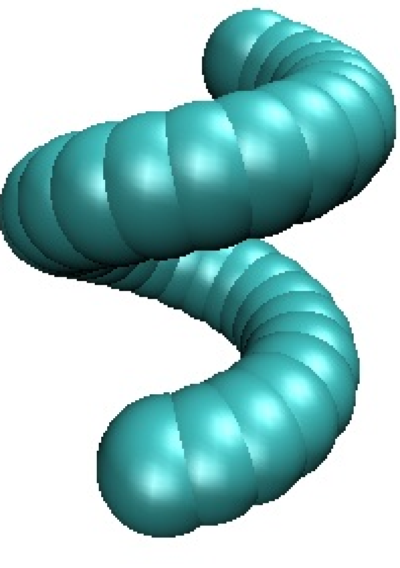
The results are plotted in Fig. 2 which include a comparison of our level-set calculation and a typical SASA type surface constructed by taking the envelope of all the LJ spheres. Though they look quite similar, our level-set result leads to a much smoother solute-solvent interface, a result from the minimization of interface area based on the energy functional.


From our MD simulations, we estimate solvation free energies of and for the alkanes A and B, respectively. The energies are positive and small and have the same order of magnitude as the solvation energy of small alkanes [36, 37]. These relatively small free energies are a well-known consequence of enthalpy-entropy compensation in the solvation of nonpolar solutes [36, 37]. It has been shown that can be decomposed in solute-solvent enthalpy and solute-solvent entropy , while the solvent-solvent enthalpy and entropy exactly cancel each other [36, 37]. For nonpolar solutes the enthalpic part is the (ensemble-averaged) total solute-solvent LJ interaction which we estimate by our MD simulations to be a large -107 and -55 for the alkanes A and B, respectively, indicating solute-solvent entropies of the same order of magnitude.
In the level-set method, we can reproduce the total solvation free energy for both alkanes within 5% by using a Tolman length of Å. In our implicit model, we can identify the solute-solvent enthalpic part by the LJ term and the entropic part by the interfacial term in the free energy functional; we find large values of and for helix A, and and for helix B, close to the values obtained by the MD simulations. We note that small variations of the Tolman length have a negligible effect on the enthalpic part of the free energy while its influence on the entropic (interfacial) part is noticeable. For example, we find for helix B when using Å instead of for Å. As the total solvation free energy is a difference of two large quantities, the interfacial part of the free energy functional (1), in particular the curvature correction, has to be reconsidered carefully.
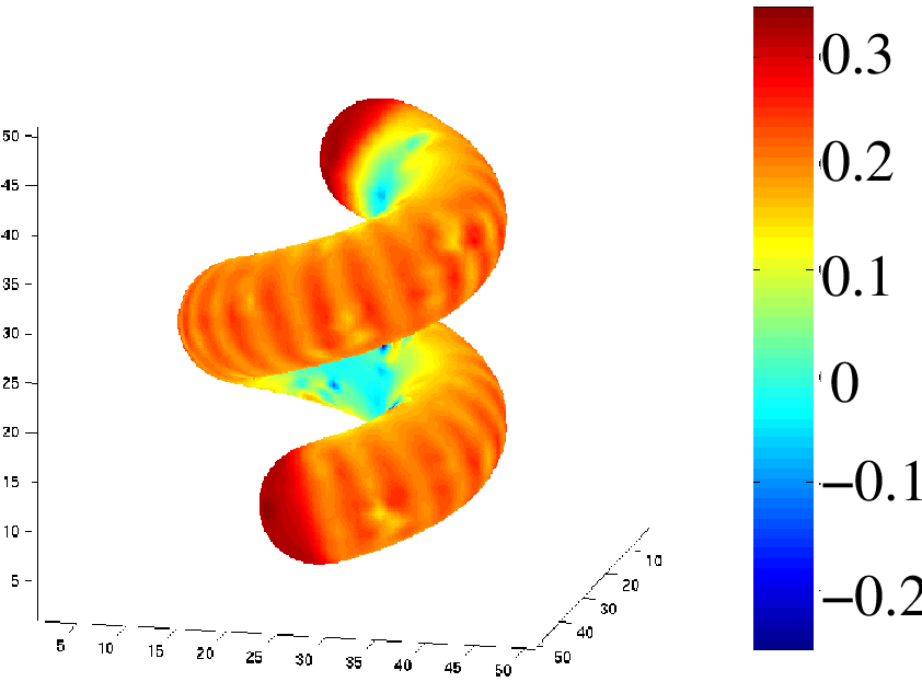
In Fig. 3, we show the same two helical chains but using a color code that indicates the value of mean curvature at each point of the solute-solvent interface. The curvature varies between positive and negative values, showing as well concave parts (blue). The highest positive curvature (deep red) is roughly given by the inverse of the length of one LJ sphere. Note that the concave parts of the loosely packed helix are within the helical core in contrast to the convex outer parts. This qualitatively different hydration of the helix depending on the local (convex or concave) geometry is in line with structural studies of water at protein-water interfaces [38].

These examples show that complex shapes with varying interface curvature, as typical in protein structures, can be efficiently tackled by the variational implicit solvent model in conjunction with the level-set method. The solute-solvent interface and the resulting energies seem to be well described by our methods, in particular when regarding the fact that the solvation free energy is a difference of large entropic and enthalpic contributions which often leads to a large error in the calculation of the total solvation free energy.
IV.3 A single molecule of fullerenes
Another interesting molecule which can be reasonably modeled as a nonpolar entity is the C60 molecule, the buckyball. The C-atom-water LJ parameters are taken from [39] and are also shown in Tab. I. The experimental solvation free energy in water is typically close to zero [40] in agreement with our MD simulations which yield . Previous more empirical implicit solvent studies show that the large interfacial energy penalty is more than compensated by the strong dispersion attraction between the water and the tightly packed carbon shell resulting in a small and negative total solvation free energy [40]. A related unusual repulsive solvent-mediated interaction between two C60 molecules has been observed in MD simulations [41].
Our level-set result for the equilibrium interface is shown in Fig. 4, featuring a smooth soccer-like surface. Using a Tolman length of Å, we can reproduce the MD solvation energy within 5%. A separate analysis of the interfacial energy part and the dispersion part shows that a large is gained from dispersion attraction while surface energy is paid. Our MD simulations confirm this cancellation of energy contributions quantitatively by showing enthalpic and entropic contributions of and , respectively.

In Fig. 5, we show the same molecule obtained by our level-set calculation with a color code that indicates the value of mean curvature of the interface. In contrast to the helical molecules, we find only convex curvatures varying from zero to roughly the inverse of the LJ size of one C atom. The curvature distribution displays the typical five and sixfold structure of the C60 molecule.

As in the previous case of the two helical alkanes, this example demonstrates that the subtle balance between interface (entropic) and dispersion (enthalpic) terms, and thus the correct interface location and curvature are crucial for an accurate description of solvation free energies, and are well captured by our methods.
IV.4 Two parallel nanometer-sized paraffin plates
In our last example, we consider the strongly hydrophobic system of two parallel paraffin plates as investigated in the explicit water MD simulations by Koishi et al. [42]. Each plate consists of fixed CH2-atoms with atom-water LJ parameters from the OPLS-AA force field, see Tab. 1, and has a square length of 3nm. The two plates are placed in a center-to-center distance and different separations are investigated. Koishi et al. observed a clear dewetting transition (vapor bubble or “nanobubble” formation) for distances Å accompanied by a strong attractive interaction energy of the order of tens of . The pmf is shown in Fig. 6 together with the solution of our variational implicit solvent model and level-set snapshots of the equilibrium interface at selected distances.

As can be seen in Fig. 6, we have almost perfect agreement with the MD simulation results. We find that the curve hardly depends on the particular choice of the Tolman length (Å here). The reason is that the average radius of mean curvature for this large-scale example is much bigger than the typical value of the Tolman length and the theory basically becomes fit-parameter free. As another important result, our variational implicit solvent model captures the nanobubble formation, see the interface snapshots in Fig. 6 for Å, a consequence of the energetic desire of the system to minimize the total interface area. For larger distances the interface breaks, i.e., the bubble ruptures and the equilibrium interface is given by two isolated plates having almost no mutual interaction.
We note here that for distances Å where bubble formation takes place, the free energy of the system might have a second, local minimum corresponding to the wetted case with two isolated plates [10]. The existence of two local minima shows the possibility of hysteresis in bubble formation as observed in the MD simulations [42].
V Conclusions and outlook
We have developed a level-set method for numerically capturing stable solute-solvent interfaces for complex shaped nonpolar molecules in three dimensions based on a recently developed variational implicit solvent model. This method evolves an arbitrary initial surface to decrease the solvation free energy until a stable equilibrium solute-solvent interface is reached.
In implementing our numerical method, we have developed a regularizing technique to stabilize the surface evolution governed geometrically by a combination of both the mean curvature and Gaussian curvature. We have additionally developed a stable, two-grid method for the calculation of the total free energy.
We have applied our method to several nonpolar systems. Our numerical results show good agreement with MD simulations with reasonable interface shapes and curvatures. In particular, due to the numerical robustness and ability of handling topological changes, our method captures the volume fusion/break and nanobubble formation/rupture in the two xenon system and the strongly hydrophobic two-plate system, respectively.
A comment is needed for the treatment of large concave curvatures which can occur locally in microscopic systems. In the two Xe atom example immediately before break-up, a singularity near the neck of the two spheres develops and can artificially increase the energy. We find that the energy is lowered if we renormalize the Tolman length for very large mean curvatures. Mathematically, it is known that even the motion of surface solely by mean curvature can induce the neck-pinch singularity that we see in our level-set calculations [43]. Therefore, it remains to be further investigated how the singularity should be treated in the free energy definition and level-set calculation.
We emphasize that our level-set implicit solvent calculations are one or two orders of magnitude faster than explicit MD simulations. Our method does require the solution of the level-set equation (12) with the normal velocity (15) in each time step. Compared with a SASA type approach, this is an “extra” work, but can be done efficiently. For instance, if we start with an initial surface that is close to an equilibrium one, our calculations can be much more efficient. With a good initial guess and a reasonable grid size, we need about – minutes to run our code for the calculation of a helical polymer chain. When the level-set method is applied to real dynamics calculations using continuum models, the relaxation of the surface to a complete equilibrium is not necessary, and only a few iterations are enough to update an interface. Therefore, in such a case, the level-set calculation can be compatible with a SASA type method in terms of efficiency.
Our level-set method can be used for the force calculation of an underlying solvation system. In principle, forces are obtained by the gradient of the free energy with respect to some spatial coordinates. One such coordinate is the geometrical location of an equilibrium solute-solvent interface. Our artificial or optimization normal velocity is exactly the effective force with respect to such a coordinate. This replaces the calculation of surface area in a SASA type method. Within the framework of level-set method, we can also evaluate forces between the solute atoms that can be used as input to Brownian dynamics computer simulations. This is an important issue that we are still investigating in details.
Finally, let us comment on further developments which will be crucial
for a complete implicit solvation description of large biomolecules by
our method. We are currently developing a level-set method for
capturing numerically stable solute-solvent interfaces using the Gibbs
free energy (1) that includes the electrostatic
contribution of the polar groups of the solutes. This method couples
the presented level-set method to a finite-difference based solver for
the Poisson-Boltzmann (PB) equation, a typical approach for the
implicit treatment of electrostatics in solvated molecular systems
[6, 7]. In [29], we derive the
variation of the free energy (1) including electrostatics
on the PB level with respect to the change of the interface
. This will be used to define the normal velocity
similar to that in (14) but extended to local electrostatic
pressures. Currently we are also developing fast and optimized level-set
methods for the handling of large systems that can have a few thousand
atoms in solutes and that can allow solute atoms to freely move around
in the optimization process. Another challenge is to extend the level-set
treatment to predict the correct dynamics of evolution of the
interface [44] and account for interface
fluctuations.
Acknowledgments. This work is partially supported by the NSF through grant DMS-0511766 (L.-T.C.) and DMS-0451466 (B.L.), by the DOE through grant DE-FG02-05ER25707 (B.L.), and by a Sloan Fellowship (L.-T.C.). J.D. thanks the Deutsche Forschungsgemeinschaft (DFG) for support within the Emmy-Noether Programme. Work in the McCammon group is supported in part by NSF, NIH, HHMI, CTBP, NBCR, and Accelrys. The authors thank Dr. Jianwei Che of Genomics Institute of the Novartis Research Foundation for useful discussions and Dr. Dietmar Paschek for making the MD data in Fig. 1 available.
References
- [1] B. Roux and T. Simonson, Biophys. Chem. 78, 1 (1999).
- [2] M. Feig and C. L. Brooks III, Current Opinion in Structure Biology 14, 217 (2004).
- [3] B. Lee and F. M. Richards, J. Mol. Biol. 55, 379 (71).
- [4] F. M. Richards, Annu. Rev. Biophys. Bioeng. 6, 151 (1977).
- [5] F. Fixman, J. Chem. Phys. 70, 4995 (1979).
- [6] M. E. Davis and J. A. McCammon, Chem. Rev. 90, 509 (1990).
- [7] K. A. Sharp and B. Honig, J. Phys. Chem. 94, 7684 (1990).
- [8] W. C. Still, A. Tempczyk, R. C. Hawley, and T. Hendrickson, J. Amer. Chem. Soc. 112, 6127 (1990).
- [9] D. Bashford and D. A. Case, Ann. Rev. Phys. Chem 51, 129 (2000).
- [10] K. Lum, D. Chandler, and J. D. Weeks, J. Phys. Chem. B 103, 4570 (1999).
- [11] D. Chandler, Nature 437, 640 (2005).
- [12] J. Chen and C. L. Brooks III, JACS 129, 2444 (2007).
- [13] J. Dzubiella, J. Swanson, and J. McCammon, Phys. Rev. Lett. 96, 087802 (2006a).
- [14] J. Dzubiella, J. Swanson, and J. McCammon, J. Chem. Phys. 124, 084905 (2006b).
- [15] S. Osher and J. A. Sethian, J. Comp. Phys. 79, 12 (1988).
- [16] J. A. Sethian, Level Set Methods and Fast Marching Methods (Cambridge University Press, 1999), 2nd ed.
- [17] S. Osher and R. Fedkiw, Level Set Methods and Dynamic Implicit Surfaces (Springer, New York, 2002).
- [18] T. Can, C.-I. Chen, and Y.-F. Wang, J. Molecular Graphics Modelling 25, 442 (2006).
- [19] D. G. Triezenberg and R. Zwanzig, Phys. Rev. Lett. 28, 1183 (1972).
- [20] H. Reiss, Adv. Chem. Phys. 9, 1 (1965).
- [21] R. C. Tolman, J. Chem. Phys. 17, 333 (1949).
- [22] D. M. Huang, P. L. Geissler, and D. Chandler, J. Phys. Chem. B 105, 6704 (2001).
- [23] H. Hadwiger, Vorlesungen über Inhalt, Oberfläche und Isoperimetrie (Springer-Verlag, Berlin-Göttingen-Heidelberg, 1957).
- [24] E. Kreyszig, Differential Geometry (Dover, New York, 1991).
- [25] L. Boruvka and A. W. Neumann, J. Chem. Phys. 66, 5464 (1977).
- [26] P.-M. König, R. Roth, and K. R. Mecke, Phys. Rev. Lett 93, 160601 (2004).
- [27] R. Roth, Y. Harano, and M. Kinoshita, Phys. Rev. Lett. 97, 078101 (2006).
- [28] K. A. Sharp, Biopolymers 36, 227 (1995).
- [29] J. Che, L.-T. Cheng, J. Dzubiella, B. Li, and J. A. McCammon, in preparation (2007).
- [30] H. J. C. Berendsen, J. R. Grigera, and T. P. Straatsma, J. Phys. Chem. 91, 6269 (1987).
- [31] J. Alejandre, D. J. Tildesley, and G. A. Chapela, J. Chem. Phys. 102, 4574 (1995).
- [32] W. Smith and T. R. Forester (1999), the DLPOLY_2 User Manual.
- [33] M. P. Allen and D. J. Tildesley, Computer Simulation of Liquids (Clarendon Press, 1987).
- [34] D. Paschek, J. Chem. Phys. 120, 6674 (2004).
- [35] R. C. Rizzo and W. L. Jorgensen, J. Amer. Chem. Soc. 121, 4827 (1999).
- [36] N. F. A. van der Vegt, D. Trzesniak, B. Kasumaj, and W. F. van Gunsteren, ChemPhysChem 5, 144 (2004).
- [37] E. Gallicchio, M. M. Kubo, and R. M. Levy, J. Phys. Chem. B 104, 6271 (2004).
- [38] M. Gerstein and C. Chothia, Proc. Nat. Acad. Sci. 93, 10167 (1996).
- [39] L. A. Girifalco, J. Phys. Chem. 96, 858 (1992).
- [40] E. B. Stukalin, M. V. Korobov, and N. V. Avramenko, J. Phys. Chem. B 107, 9692 (2003).
- [41] L. Li, D. Bedrov, and G. D. Smith, Phys. Rev. E 71, 011502 (2005).
- [42] T. Koishi, S. Yoo, K. Yasuoka, X. C. Zeng, T. Narumi, R. Susukita, A. Kawai, H. Furusawa, A. Suenaga, N. Okimoto, et al., Phys. Rev. Lett. 93, 185701 (2004).
- [43] S. B. Angenent and J. J. L. Velázquez, J. Reine Angew. Math. 482, 15 (1997).
- [44] J. Dzubiella, J. Chem. Phys. 126, 194504 (2007).