跳到论文正文
W Papers独立论文阅读器 arXiv:0809.0082 论文正文 计算阅读时间 · 0%
引用这篇论文根据当前论文元数据生成,正式投稿前建议核对。


License: arXiv.org perpetual non-exclusive license
arXiv:0809.0082v1 [hep-th] 30 Aug 2008

A new perspective in the dark energy puzzle from particle mixing phenomenon

M.Blasone♭, A.Capolupo♭, S.Capozziello♯, G.Vitiello♭ Affiliation: ♭ Dipartimento di Matematica e Informatica, Università di Salerno and Istituto Nazionale di Fisica Nucleare, Gruppo Collegato di Salerno, 84100 Salerno, Italy,
♯ Dipartimento di Scienze Fisiche, Università di Napoli ”Federico II” and INFN Sez. di Napoli, Compl. Univ. Monte S. Angelo, Ed.N, Via Cinthia, I-80126 Napoli, Italy.
Abstract

We report on recent results on particle mixing and oscillations in quantum field theory. We discuss the role played in cosmology by the vacuum condensate induced by the neutrino mixing phenomenon. We show that it can contribute to the dark energy of the universe.

pacs
98.80.Cq, 98.80. Hw, 04.20.Jb, 04.50+h

I Introduction

The study of neutrino mixing in the context of quantum field theory (QFT) [1, 2, 3, 4, 5, 6] and the progresses in the understanding of such a phenomenon [7, 8], together with the definitive experimental proof of neutrino oscillations [9, 10], open new scenarios to the research in fundamental physics. Indeed, it has emerged an unexpectedly rich non-perturbative structure associated to the mixing of neutrino (as well as boson [11]) fields, hidden in the vacuum for the flavor fields. This has been shown to be a condensate of massive neutrino-antineutrino pairs. Several consequences of this discovery have been analyzed, including the effects on flavor oscillation formulas [1, 5] and the implications in cosmology and astro-particle physics [12, 13, 14].

In this review we show that the energy content of the neutrino mixing vacuum condensate [12] can represent a component of dark energy [13] that, at present epoch, assumes the behavior and the value of the observed cosmological constant. We compute such a value and show that, above a threshold, it is slowly diverging and its derivative with respect to the cut-off value goes actually to zero, which allows to use the cut-off at its electroweak scale value, provided one limits himself to considering the two (lighter) generations in neutrino mixing. In the case one includes mixing with heavier neutrinos, a value of the dark energy compatible with its upper bound is obtained for a cut-off of the order of the natural scale of neutrino mixing. As we will show in a forthcoming paper [15], the use of such an infrared momentum cut-off is motivated, at the present epoch, by the negligible breaking of Lorentz invariance due to the vacuum condensate caused by neutrino mixing .

The remarkable improvement of the dark energy value computed in the present paper, with respect to the disagreement of 123123 orders of magnitude in standard approaches [16], makes the present treatment worth to be discussed.

Our result links together dark energy with the sub-eV neutrino mass scale [17]. The link comes from the neutrino-antineutrino pair vacuum condensate.

We point out that our work differs from the approach [18] based on vacuum contributions from light particles like neutrinos and axions. In the present review we do not resort to axion contributions. Nevertheless, it is in our future plan to compare the two approaches in order to clarify the differences and the similarities. Moreover, the non-perturbative feature here presented leads us to believe that a neutrino–antineutrino asymmetry, if any, related with lepton number violation [19] would not affect much our result. Also this point deserves to be better clarified, which we plan to do in a subsequent work. Finally, we observe that the non-perturbative contribution discussed in the present review is of different origin with respect to the vacuum energy contribution of massive spinor fields arising from a radiative correction at some perturbative order [20].

The review is organized as follows. In Section II, we introduce the neutrino mixing formalism in QFT. In Section III we present the neutrino mixing contribution to the dark energy of the universe. Conclusions are drawn in Section IV.

II Neutrino mixing in Quantum Field Theory

The neutrino mixing phenomenon was firstly studied in the context of quantum mechanics (QM) [21, 22, 23, 24, 25, 26, 27, 28] and subsequently analyzed in the framework of the QFT formalism [1, 2, 3, 4, 5, 6, 7, 8], which we shortly summarize in the following (for a detailed review see [6]).

In the very effective Pontecorvo’s formalism neutrino mixing is considered from the standpoint of QM and the attention is focused on the mixing of ”states”. The fact that neutrinos are actually described by field operators is completely neglected. The reason for that is the necessity of the effectiveness of the formalism which is required to readily fit the experimental search for mixing and oscillations. Therefore, any simplification of the matter to be treated is adopted, provided the resulting description would be sufficiently accurate and descriptive/predictive of the experimental observations. As a matter of fact, the successive development of the experimental search has been supporting such an attitude. From a theoretical point of view, there is, however, the necessity to understand how mixing and oscillations can be properly described in the realm of QFT, which provides anyway the proper setting for neutrino dynamics, as known since the birth of QFT. It is then also necessary to understand how the correct formalism connects to the Pontecorvo’s approximate scheme. This has been indeed the program of the research line which has led to the QFT formulation of the neutrino mixing and oscillation. Such a program has been successively extended so to incorporate other particle mixing (quark mixing, boson mixing). Here we only sketch the skeleton of the QFT mixing formalism and to do that we consider two neutrinos. Extension to three neutrino (to any number of generations, in principle) is in the literature [5]. The reader who wants the guaranties offered by a rigorous mathematical proof of our treatment may usefully read the papers in Refs.[4].

The mixing transformations for two Dirac neutrino fields are

νe​(x)\displaystyle\nu_{e}(x) =\displaystyle= ν1​(x)​cos⁡θ+ν2​(x)​sin⁡θ\displaystyle\nu_{1}(x)\,\cos\theta+\nu_{2}(x)\,\sin\theta
νμ​(x)\displaystyle\nu_{\mu}(x) =\displaystyle= −ν1​(x)​sin⁡θ+ν2​(x)​cos⁡θ,\displaystyle-\nu_{1}(x)\,\sin\theta+\nu_{2}(x)\,\cos\theta\;, (1)

where νe​(x)\nu_{e}(x) and νμ​(x)\nu_{\mu}(x) are the fields with definite flavors, θ\theta is the mixing angle and ν1\nu_{1} and ν2\nu_{2} are the fields with definite masses m1≠m2m_{1}\neq m_{2}:

νi(x)=1V∑𝐤,r[u𝐤,irα𝐤,ir(t)+v−𝐤,irβ−𝐤,ir†(t)]ei​𝐤⋅𝐱,i=1,2,\displaystyle\nu_{i}(x)=\frac{1}{\sqrt{V}}{\sum_{{\bf k},r}}\left[u^{r}_{{\bf k},i}\,\alpha^{r}_{{\bf k},i}(t)+v^{r}_{-{\bf k},i}\,\beta^{r{\dagger}}_{-{\bf k},i}(t)\right]e^{i{\bf k}\cdot{\bf x}},\qquad\,\qquad i=1,2, (2)

with α𝐤,ir​(t)=α𝐤,ir​e−i​ωk,i​t\alpha_{{\bf k},i}^{r}(t)=\alpha_{{\bf k},i}^{r}\,e^{-i\omega_{k,i}t}, β𝐤,ir†(t)=β𝐤,ir†ei​ωk,i​t,\beta_{{\bf k},i}^{r{\dagger}}(t)=\beta_{{\bf k},i}^{r{\dagger}}\,e^{i\omega_{k,i}t}, and ωk,i=𝐤2+mi2.\omega_{k,i}=\sqrt{{\bf k}^{2}+m_{i}^{2}}. The operators α𝐤,ir\alpha^{r}_{{\bf k},i} and β𝐤,ir\beta^{r}_{{\bf k},i}, i=1,2,r=1,2i=1,2\;,\;r=1,2 annihilate the vacuum state |0⟩1,2≡|0⟩1⊗|0⟩2|0\rangle_{1,2}\equiv|0\rangle_{1}\otimes|0\rangle_{2}: α𝐤,ir​|0⟩12=β𝐤,ir​|0⟩12=0\alpha^{r}_{{\bf k},i}|0\rangle_{12}=\beta^{r}_{{\bf k},i}|0\rangle_{12}=0. The anticommutation relations are: {νiα(x),νjβ†(y)}t=t′=δ3(𝐱−𝐲)δα​βδi​j,\left\{\nu_{i}^{\alpha}(x),\nu_{j}^{\beta\dagger}(y)\right\}_{t=t^{\prime}}=\delta^{3}({\bf x-y})\delta_{\alpha\beta}\delta_{ij}, with α,β=1,…​4,\alpha,\beta=1,...4, and {α𝐤,ir,α𝐪,js†}=δ𝐤𝐪δr​sδi​j;\left\{\alpha_{{\bf k},i}^{r},\alpha_{{\bf q},j}^{s\dagger}\right\}=\delta_{{\bf kq}}\delta_{rs}\delta_{ij}; {β𝐤,ir,β𝐪,js†}=δ𝐤𝐪δr​sδi​j,\left\{\beta_{{\bf k},i}^{r},\beta_{{\bf q,}j}^{s\dagger}\right\}=\delta_{{\bf kq}}\delta_{rs}\delta_{ij}, with i,j=1,2.i,j=1,2. All other anticommutators are zero. The orthonormality and completeness relations are: u𝐤,ir†u𝐤,is=v𝐤,ir†v𝐤,is=δr​s,u_{{\bf k},i}^{r\dagger}u_{{\bf k},i}^{s}=v_{{\bf k},i}^{r\dagger}v_{{\bf k},i}^{s}=\delta_{rs},\; u𝐤,ir†v−𝐤,is=v−𝐤,ir†u𝐤,is=0,u_{{\bf k},i}^{r\dagger}v_{-{\bf k},i}^{s}=v_{-{\bf k},i}^{r\dagger}u_{{\bf k},i}^{s}=0,\; and ∑r(u𝐤,iru𝐤,ir†+v−𝐤,irv−𝐤,ir†)=1.\sum_{r}(u_{{\bf k},i}^{r}u_{{\bf k},i}^{r\dagger}+v_{-{\bf k},i}^{r}v_{-{\bf k},i}^{r\dagger})=1.

The mixing transformation Eqs.(1) can be written as [1]:

νeα​(x)=Gθ−1​(t)​ν1α​(x)​Gθ​(t)\displaystyle\nu_{e}^{\alpha}(x)=G^{-1}_{\bf\theta}(t)\;\nu_{1}^{\alpha}(x)\;G_{\bf\theta}(t) (3)
νμα​(x)=Gθ−1​(t)​ν2α​(x)​Gθ​(t)\displaystyle\nu_{\mu}^{\alpha}(x)=G^{-1}_{\bf\theta}(t)\;\nu_{2}^{\alpha}(x)\;G_{\bf\theta}(t)

where the mixing generator Gθ​(t)G_{\bf\theta}(t) is given by

Gθ​(t)=e​x​p​[θ​∫d3​𝐱​(ν1†​(x)​ν2​(x)−ν2†​(x)​ν1​(x))].\displaystyle G_{\bf\theta}(t)=exp\left[\theta\int d^{3}{\bf x}\left(\nu_{1}^{{\dagger}}(x)\nu_{2}(x)-\nu_{2}^{{\dagger}}(x)\nu_{1}(x)\right)\right]\,. (4)

At finite volume, Gθ​(t)G_{\bf\theta}(t) is an unitary operator, Gθ−1​(t)=G−θ​(t)=Gθ†​(t)G^{-1}_{\bf\theta}(t)=G_{\bf-\theta}(t)=G^{{\dagger}}_{\bf\theta}(t), preserving the canonical anticommutation relations; Gθ−1​(t)G^{-1}_{\bf\theta}(t) maps the Hilbert spaces for ν1\nu_{1} and ν2\nu_{2} fields ℋ1,2{\cal H}_{1,2} to the Hilbert spaces for flavored fields ℋe,μ{\cal H}_{e,\mu}: Gθ−1​(t):ℋ1,2↦ℋe,μ.G^{-1}_{\bf\theta}(t):{\cal H}_{1,2}\mapsto{\cal H}_{e,\mu}. In particular, for the vacuum |0⟩1,2|0\rangle_{1,2} we have, at finite volume VV:

|0​(t)⟩e,μ=Gθ−1​(t)​|0⟩1,2.\displaystyle|0(t)\rangle_{e,\mu}=G^{-1}_{\bf\theta}(t)\;|0\rangle_{1,2}\,. (5)

|0⟩e,μ|0\rangle_{e,\mu} is the vacuum for ℋe,μ{\cal H}_{e,\mu}, which we will refer to as the flavor vacuum. The explicit expression for |0⟩e,μ|0\rangle_{e,\mu} at time t=0t=0 in the reference frame for which 𝐤=(0,0,|𝐤|){\bf k}=(0,0,|{\bf k}|) is

|0⟩e,μ\displaystyle|0\rangle_{e,\mu} =\displaystyle= ∏r,𝐤[(1−sin2θ|V𝐤|2)−ϵrsinθcosθ|V𝐤|(α𝐤,1r†β−𝐤,2r†+α𝐤,2r†β−𝐤,1r†)+\displaystyle\prod_{r,{\bf k}}\Big[(1-\sin^{2}\theta\;|V_{{\bf k}}|^{2})-\epsilon^{r}\sin\theta\;\cos\theta\;|V_{{\bf k}}|(\alpha^{r{\dagger}}_{{\bf k},1}\beta^{r{\dagger}}_{-{\bf k},2}+\alpha^{r{\dagger}}_{{\bf k},2}\beta^{r{\dagger}}_{-{\bf k},1})+ (6)
+\displaystyle+ ϵrsin2θ|V𝐤||U𝐤|(α𝐤,1r†β−𝐤,1r†−α𝐤,2r†β−𝐤,2r†)+sin2θ|V𝐤|2α𝐤,1r†β−𝐤,2r†α𝐤,2r†β−𝐤,1r†]|0⟩1,2.\displaystyle\epsilon^{r}\sin^{2}\theta\;|V_{{\bf k}}||U_{{\bf k}}|(\alpha^{r{\dagger}}_{{\bf k},1}\beta^{r{\dagger}}_{-{\bf k},1}-\alpha^{r{\dagger}}_{{\bf k},2}\beta^{r{\dagger}}_{-{\bf k},2})+\sin^{2}\theta\;|V_{{\bf k}}|^{2}\alpha^{r{\dagger}}_{{\bf k},1}\beta^{r{\dagger}}_{-{\bf k},2}\alpha^{r{\dagger}}_{{\bf k},2}\beta^{r{\dagger}}_{-{\bf k},1}\Big]|0\rangle_{1,2}\,.

Eq.(6) exhibits the condensate structure of the flavor vacuum |0⟩e,μ|0\rangle_{e,\mu}. The important point is that ⟨0|0(t)⟩e,μ1,2→0{}_{1,2}\langle 0|0(t)\rangle_{e,\mu}\rightarrow 0, for any tt, in the infinite volume limit [1]. Thus, in such a limit the Hilbert spaces ℋ1,2{\cal H}_{1,2} and ℋe,μ{\cal H}_{e,\mu} turn out to be unitarily inequivalent spaces. We remark that |0⟩e,μ|0\rangle_{e,\mu} is the physical vacuum as we will see below.

In the QM formalism we ”cannot” have two unitarily inequivalent Hilbert spaces for the simple reason that the von Neumann theorem forbids the existence of unitarily inequivalent representations of the canonical (anti-)commutation rules whenever the system has a finite number of degrees of freedom, such as those in QM. It is quite obvious that this cannot be the case for neutrinos. Since they are quantum fields, by definition they are described by infinitely many degrees of freedom and thus von Neumann theorem does not hold. This point introduces a crucial difference between the QFT formalism and the QM approach.

The flavor annihilators, relative to the fields νe​(x)\nu_{e}(x) and νμ​(x)\nu_{\mu}(x) at each time, are given by (we use (σ,i)=(e,1),(μ,2)(\sigma,i)=(e,1),(\mu,2)):

α𝐤,σr​(t)\displaystyle\alpha_{{\bf k},\sigma}^{r}(t) ≡\displaystyle\equiv Gθ−1​(t)​α𝐤,ir​(t)​Gθ​(t),\displaystyle G^{-1}_{\bf\theta}(t)\;\alpha_{{\bf k},i}^{r}(t)\;G_{\bf\theta}(t)\,,
β𝐤,σr​(t)\displaystyle\beta_{{\bf k},\sigma}^{r}(t) ≡\displaystyle\equiv Gθ−1​(t)​β𝐤,ir​(t)​Gθ​(t).\displaystyle G^{-1}_{\bf\theta}(t)\;\beta_{{\bf k},i}^{r}(t)\;G_{\bf\theta}(t)\,. (7)

The flavor fields can be expanded in the same bases as νi\nu_{i}:

νσ​(𝐱,t)\displaystyle\nu_{\sigma}({\bf x},t) =\displaystyle= 1V∑𝐤,rei​𝐤.𝐱[u𝐤,irα𝐤,σr(t)+v−𝐤,irβ−𝐤,σr†(t)].\displaystyle\frac{1}{\sqrt{V}}{\sum_{{\bf k},r}}e^{i{\bf k.x}}\left[u_{{\bf k},i}^{r}\alpha_{{\bf k},\sigma}^{r}(t)+v_{-{\bf k},i}^{r}\beta_{-{\bf k},\sigma}^{r\dagger}(t)\right]\,. (8)

The flavor annihilation operators in the reference frame such that 𝐤=(0,0,|𝐤|){\bf k}=(0,0,|{\bf k}|) are:

α𝐤,er​(t)\displaystyle\alpha^{r}_{{\bf k},e}(t) =\displaystyle= cosθα𝐤,1r(t)+sinθ(|U𝐤|α𝐤,2r(t)+ϵr|V𝐤|β−𝐤,2r†(t))\displaystyle\cos\theta\;\alpha^{r}_{{\bf k},1}(t)\;+\;\sin\theta\;\left(|U_{{\bf k}}|\;\alpha^{r}_{{\bf k},2}(t)\;+\;\epsilon^{r}\;|V_{{\bf k}}|\;\beta^{r{\dagger}}_{-{\bf k},2}(t)\right)
α𝐤,μr​(t)\displaystyle\alpha^{r}_{{\bf k},\mu}(t) =\displaystyle= cosθα𝐤,2r(t)−sinθ(|U𝐤|α𝐤,1r(t)−ϵr|V𝐤|β−𝐤,1r†(t))\displaystyle\cos\theta\;\alpha^{r}_{{\bf k},2}(t)\;-\;\sin\theta\;\left(|U_{{\bf k}}|\;\alpha^{r}_{{\bf k},1}(t)\;-\;\epsilon^{r}\;|V_{{\bf k}}|\;\beta^{r{\dagger}}_{-{\bf k},1}(t)\right)
β−𝐤,er​(t)\displaystyle\beta^{r}_{-{\bf k},e}(t) =\displaystyle= cosθβ−𝐤,1r(t)+sinθ(|U𝐤|β−𝐤,2r(t)−ϵr|V𝐤|α𝐤,2r†(t))\displaystyle\cos\theta\;\beta^{r}_{-{\bf k},1}(t)\;+\;\sin\theta\;\left(|U_{{\bf k}}|\;\beta^{r}_{-{\bf k},2}(t)\;-\;\epsilon^{r}\;|V_{{\bf k}}|\;\alpha^{r{\dagger}}_{{\bf k},2}(t)\right) (9)
β−𝐤,μr​(t)\displaystyle\beta^{r}_{-{\bf k},\mu}(t) =\displaystyle= cosθβ−𝐤,2r(t)−sinθ(|U𝐤|β−𝐤,1r(t)+ϵr|V𝐤|α𝐤,1r†(t)),\displaystyle\cos\theta\;\beta^{r}_{-{\bf k},2}(t)\;-\;\sin\theta\;\left(|U_{{\bf k}}|\;\beta^{r}_{-{\bf k},1}(t)\;+\;\epsilon^{r}\;|V_{{\bf k}}|\;\alpha^{r{\dagger}}_{{\bf k},1}(t)\right),

where ϵr=(−1)r\epsilon^{r}=(-1)^{r} and

|U𝐤|≡ur†𝐤,iur𝐤,j=vr†−𝐤,ivr−𝐤,j,i≠j;|V𝐤|≡εi​jϵrur†𝐤,ivr−𝐤,j,nosummation\displaystyle|U_{{\bf k}}|\equiv u^{r{\dagger}}_{{\bf k},i}u^{r}_{{\bf k},j}=v^{r{\dagger}}_{-{\bf k},i}v^{r}_{-{\bf k},j}\,,\qquad i\neq j\,;\qquad\qquad|V_{{\bf k}}|\equiv\varepsilon_{ij}\epsilon^{r}\;u^{r{\dagger}}_{{\bf k},i}v^{r}_{-{\bf k},j},\quad{\rm no\,\,summation} (10)

with εi​j=0,1,−1\varepsilon_{ij}=0,1,-1 for i=j,i⁡<j,i>​ji=j,\penalty\ i<j,\penalty\ i>j, respectively. We have:

|U𝐤|=(ωk,1+m12​ωk,1)12​(ωk,2+m22​ωk,2)12​(1+𝐤2(ωk,1+m1)​(ωk,2+m2))\displaystyle|U_{{\bf k}}|=\left(\frac{\omega_{k,1}+m_{1}}{2\omega_{k,1}}\right)^{\frac{1}{2}}\left(\frac{\omega_{k,2}+m_{2}}{2\omega_{k,2}}\right)^{\frac{1}{2}}\left(1+\frac{{\bf k}^{2}}{(\omega_{k,1}+m_{1})(\omega_{k,2}+m_{2})}\right)
|V𝐤|=(ωk,1+m12​ωk,1)12​(ωk,2+m22​ωk,2)12​(k(ωk,2+m2)−k(ωk,1+m1))\displaystyle|V_{{\bf k}}|=\left(\frac{\omega_{k,1}+m_{1}}{2\omega_{k,1}}\right)^{\frac{1}{2}}\left(\frac{\omega_{k,2}+m_{2}}{2\omega_{k,2}}\right)^{\frac{1}{2}}\left(\frac{k}{(\omega_{k,2}+m_{2})}-\frac{k}{(\omega_{k,1}+m_{1})}\right) (11)
|U𝐤|2+|V𝐤|2=1.\displaystyle|U_{{\bf k}}|^{2}+|V_{{\bf k}}|^{2}=1\,. (12)

The number of condensate neutrinos for each 𝐤\bf k is given by

⟨0|α𝐤,ir†α𝐤,ir|0⟩e,μe,μ=e,μ⟨0|β𝐤,ir†β𝐤,ir|0⟩e,μ=sin2θ|V𝐤|2,{}_{e,\mu}\langle 0|\alpha_{{\bf k},i}^{r{\dagger}}\alpha^{r}_{{\bf k},i}|0\rangle_{e,\mu}\,=\;_{e,\mu}\langle 0|\beta_{{\bf k},i}^{r{\dagger}}\beta^{r}_{{\bf k},i}|0\rangle_{e,\mu}\,=\,\sin^{2}\theta\;|V_{{\bf k}}|^{2}\;, (13)

with i=1,2i=1,2\,. Equivalently, ⟨0|α𝐤,σr†α𝐤,σr|0⟩1,21,2=1,2⟨0|β𝐤,σr†β𝐤,σr|0⟩1,2=sin2θ|V𝐤|2,{}_{1,2}\langle 0|\alpha_{{\bf k},\sigma}^{r{\dagger}}\alpha^{r}_{{\bf k},\sigma}|0\rangle_{1,2}\,=\;_{1,2}\langle 0|\beta_{{\bf k},\sigma}^{r{\dagger}}\beta^{r}_{{\bf k},\sigma}|0\rangle_{1,2}\,=\,\sin^{2}\theta\;|V_{{\bf k}}|^{2}\;, with σ=e,μ\sigma=e,\mu\,.

The Bogoliubov coefficient |V𝐤|2|V_{{\bf k}}|^{2} appearing in Eq.(13) can be written as a function of the dimensionless momentum p=|𝐤|m1​m2p=\frac{|{\bf k}|}{\sqrt{m_{1}m_{2}}} and dimensionless parameter a=(m2−m1)2m1​m2a=\frac{(m_{2}-m_{1})^{2}}{m_{1}m_{2}}, as follows,

|V⁡(p,a)|2\displaystyle|V(p,a)|^{2} =\displaystyle= 12​(1−p2+1(p2+1)2+a​p2).\displaystyle\frac{1}{2}\left(1-\frac{p^{2}+1}{\sqrt{(p^{2}+1)^{2}+ap^{2}}}\right)\penalty\ . (14)

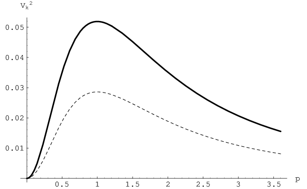
From Fig.1 we see that the effect is maximal when p=1p=1, i.e. for |𝐤|2=m1​m2|{\bf k}|^{2}=m_{1}m_{2}, the natural scale of the neutrino mixing. |V𝐤|2|V_{{\bf k}}|^{2} goes to zero for large momenta, i.e. for |𝐤|2≫m1​m2|{\bf k}|^{2}\gg m_{1}m_{2}, as |V𝐤|2≈(Δ​m)24​k2|V_{{\bf k}}|^{2}\approx\frac{(\Delta m)^{2}}{4k^{2}}. It acts as a “form factor” in the 𝐤\bf k space controlling the neutrino vacuum condensate. We thus find that the Pontecorvo’s formalism is nothing but the relativistic limit of the QFT formalism: |V𝐤|2→0|V_{{\bf k}}|^{2}\rightarrow 0 and |U𝐤|2→1|U_{{\bf k}}|^{2}\rightarrow 1 for |𝐤|2≫m1​m2|{\bf k}|^{2}\gg m_{1}m_{2}. In the Pontecorvo’s formalism the non-perturbative contributions from the vacuum condensate are thus missing. This is the meaning of the approximation made in the QM treatment of the mixing. Missing these condensate contributions is of course of no relevance for the experimental observation of neutrino oscillations at today instrumentation resolution. These contributions might play, however, a relevant role in the study of the cosmological background. The fact that |V𝐤|2|V_{{\bf k}}|^{2} contributes maximally for low energies suggests indeed to us that the contribution of the mixing phenomenon may be taken as a good candidate in the study of dark energy.
Refer to caption
Figure 1: The fermion condensation density |V⁡(p,a)|2|V(p,a)|^{2} as a function of pp for a=0.98a=0.98 (solid line) and a=0.5a=0.5 (dashed line).

We point out that, since |0⟩1,2|0\rangle_{1,2} and |0⟩e,μ|0\rangle_{e,\mu} are unitary inequivalent states in the infinite volume limit, two different normal orderings must be defined, respectively with respect to the vacuum |0⟩1,2|0\rangle_{1,2} for fields with definite masses, denoted as usual by :…::...:, and with respect to the vacuum for fields with definite flavor |0⟩e,μ|0\rangle_{e,\mu}, denoted by ::…::::...:: . The Hamiltonian normal ordered with respect to the vacuum |0⟩1,2|0\rangle_{1,2}\, is given by

:H:=H−1,2⟨0|H|0⟩1,2=H+ 2∫d3𝐤(ωk,2+ωk,1)=∑i∑r∫d3𝐤ωk,i[α𝐤,ir†α𝐤,ir+β𝐤,ir†β𝐤,ir],\displaystyle:H:\,=\,H-_{1,2}\langle 0|H|0\rangle_{1,2}=H+\,2\int d^{3}{\bf k}\,(\omega_{k,2}+\omega_{k,1})=\sum_{i}\sum_{r}\int d^{3}{\bf k}\,\omega_{k,i}[\alpha_{{\bf k},i}^{r{\dagger}}\alpha_{{\bf k},i}^{r}+\beta_{{\bf k},i}^{r{\dagger}}\beta_{{\bf k},i}^{r}]\penalty\ , (15)

and the Hamiltonian normal ordered with respect to the vacuum |0⟩e,μ|0\rangle_{e,\mu} is

::H::≡H−⟨0(t)|H|0(t)⟩e,μe,μ=H+ 2∫d3𝐤(ωk,2+ωk,1)(1−2|V𝐤|2sin2θ).\displaystyle:\;\!\!\;\!\!:H:\;\!\!\;\!\!:\,\equiv\,H\,-\,{}_{e,\mu}\langle 0(t)|H|0(t)\rangle_{e,\mu}\,=H\,+\,2\int d^{3}{\bf k}\,(\omega_{k,2}+\omega_{k,1})\,(1-2\,|V_{\bf k}|^{2}\sin^{2}\theta)\,. (16)

Note that the difference of energy between |0⟩e,μ|0\rangle_{e,\mu} and |0⟩1,2|0\rangle_{1,2} represents the energy of the condensed neutrinos given in Eq.(13)

⟨0(t)|:H:|0(t)⟩e,μe,μ=⟨0(t)|H|0(t)⟩e,μe,μ−⟨0|H|0⟩1,21,2= 4sin2θ∫d3𝐤(ωk,2+ωk,1)|V𝐤|2,\displaystyle{}_{e,\mu}\langle 0(t)|:H:|0(t)\rangle_{e,\mu}\,=\,{}_{e,\mu}\langle 0(t)|H|0(t)\rangle_{e,\mu}\,-\,{}_{1,2}\langle 0|H|0\rangle_{1,2}\,=\,4\,\sin^{2}\theta\,\int d^{3}{\bf k}\,(\omega_{k,2}+\omega_{k,1})\,|V_{\bf k}|^{2}\penalty\ , (17)

and gives the “energy gap” protecting the flavored neutrinos from turning into the mixing component neutrinos ν1\nu_{1} and ν2\nu_{2}. In the following we show that the energy of the condensed neutrinos can have cosmological implications, indeed it can contribute to the dark energy of the universe.

Before considering cosmological aspects of neutrino mixing, in order to better understand the meaning of Eq.(17), let us introduce the operator A⁡(t)A(t) that satisfies Eqs.(39) - (42) given in Appendix A. By defining the operator

H′​(t)=:H:−A⁡(t),\displaystyle H^{\prime}(t)\,=\,:H:-A(t)\,, (18)

we have

⟨ν𝐤,er​(t)|H′​(t)|ν𝐤,er​(t)⟩\displaystyle\langle\nu_{{\bf k},e}^{r}(t)|\,H^{\prime}(t)\,|\nu_{{\bf k},e}^{r}(t)\rangle =\displaystyle= ωk,1​cos2⁡θ+ωk,2​sin2⁡θ,\displaystyle\omega_{k,1}\cos^{2}\theta\,+\omega_{k,2}\sin^{2}\theta\,, (19)
⟨ν𝐤,μr​(t)|H′​(t)|ν𝐤,μr​(t)⟩\displaystyle\langle\nu_{{\bf k},\mu}^{r}(t)|\,H^{\prime}(t)\,|\nu_{{\bf k},\mu}^{r}(t)\rangle =\displaystyle= ωk,2​cos2⁡θ+ωk,1​sin2⁡θ,\displaystyle\ \omega_{k,2}\cos^{2}\theta\,+\omega_{k,1}\sin^{2}\theta\,, (20)
⟨ν𝐤,er​(t)|H′​(t)|ν𝐤,μr​(t)⟩\displaystyle\langle\nu_{{\bf k},e}^{r}(t)|\,H^{\prime}(t)\,|\nu_{{\bf k},\mu}^{r}(t)\rangle =\displaystyle= (ωk,2−ωk,1)​sin⁡θ​cos⁡θ,\displaystyle(\omega_{k,2}-\omega_{k,1})\sin\theta\cos\theta\,, (21)
⟨ν𝐤,μ​e¯​er​(t)|H′​(t)|ν𝐤,er​(t)⟩=⟨ν𝐤,μ​e¯​er​(t)|H′​(t)|ν𝐤,μr​(t)⟩=⟨ν𝐤,e​μ¯​μr​(t)|H′​(t)|ν𝐤,er​(t)⟩=⟨ν𝐤,e​μ¯​μr​(t)​|H′​(t)|​ν𝐤,μr​(t)⟩=0.\displaystyle\langle\nu_{{\bf k},\mu\bar{e}e}^{r}(t)|\,H^{\prime}(t)\,|\nu_{{\bf k},e}^{r}(t)\rangle\,=\,\langle\nu_{{\bf k},\mu\bar{e}e}^{r}(t)|\,H^{\prime}(t)\,|\nu_{{\bf k},\mu}^{r}(t)\rangle\,=\,\langle\nu_{{\bf k},e\bar{\mu}\mu}^{r}(t)|\,H^{\prime}(t)\,|\nu_{{\bf k},e}^{r}(t)\rangle\,=\,\langle\nu_{{\bf k},e\bar{\mu}\mu}^{r}(t)|\,H^{\prime}(t)\,|\nu_{{\bf k},\mu}^{r}(t)\rangle=0\,.

Eqs.(19)-(21) coincide with the ones obtained in QM by using the Pontecorvo states. Moreover the uncertainties in the energy H′​(t)H^{\prime}(t) of the multi-particle states (43), (44) are zero such as in QM, are zero the uncertainties in the energy HH of the multi-particle states. H′​(t)H^{\prime}(t) is explicitly given by

H′​(t)\displaystyle H^{\prime}(t) =\displaystyle= ∑r∫d3𝐤[ωe​e(α𝐤,er†(t)α𝐤,er(t)+β−𝐤,er†(t)β−𝐤,er(t))+ωμ​μ(α𝐤,μr†(t)α𝐤,μr(t)+β−𝐤,μr†(t)β−𝐤,μr(t))\displaystyle\sum_{r}\int d^{3}{\bf k}\,\Big[\omega_{ee}\left(\alpha_{{\bf k},e}^{r{\dagger}}(t)\alpha_{{\bf k},e}^{r}(t)\,+\,\beta_{-{\bf k},e}^{r{\dagger}}(t)\beta_{-{\bf k},e}^{r}(t)\right)\,+\,\omega_{\mu\mu}\left(\alpha_{{\bf k},\mu}^{r{\dagger}}(t)\alpha_{{\bf k},\mu}^{r}(t)+\beta_{-{\bf k},\mu}^{r{\dagger}}(t)\beta_{-{\bf k},\mu}^{r}(t)\right) (23)
+\displaystyle+ ωμ​e(α𝐤,er†(t)α𝐤,μr(t)+α𝐤,μr†(t)α𝐤,er(t)+β−𝐤,er†(t)β−𝐤,μr(t)+β−𝐤,μr†(t)β𝐤,er(t))],\displaystyle\omega_{\mu e}\left(\alpha_{{\bf k},e}^{r{\dagger}}(t)\alpha_{{\bf k},\mu}^{r}(t)\,+\,\alpha_{{\bf k},\mu}^{r{\dagger}}(t)\alpha_{{\bf k},e}^{r}(t)\,+\,\beta_{-{\bf k},e}^{r{\dagger}}(t)\beta_{-{\bf k},\mu}^{r}(t)\,+\,\beta_{-{\bf k},\mu}^{r{\dagger}}(t)\beta_{{\bf k},e}^{r}(t)\right)\Big]\,,

where ωe​e≡ωk,1​cos2⁡θ+ωk,2​sin2⁡θ\omega_{ee}\equiv\omega_{k,1}\,\cos^{2}\theta\,+\omega_{k,2}\,\sin^{2}\theta, ωμ​μ≡ωk,1​sin2⁡θ+ωk,2​cos2⁡θ\omega_{\mu\mu}\equiv\omega_{k,1}\,\sin^{2}\theta\,+\omega_{k,2}\,\cos^{2}\theta, ωμ​e≡(ωk,2−ωk,1)​sin⁡θ​cos⁡θ\omega_{\mu e}\equiv(\omega_{k,2}-\omega_{k,1})\,\sin\theta\cos\theta. From Eq.(23) we have at any time tt

⟨0(t)|H′(t)|0(t)⟩e,μe,μ= 0.\displaystyle{}_{e,\mu}\langle 0(t)|H^{\prime}(t)|0(t)\rangle_{e,\mu}\,=\,0\,. (24)

Thus we obtain

⟨0(t)|:H:|0(t)⟩e,μe,μ≡⟨0(t)|A(t)|0(t)⟩e,μe,μ.\displaystyle{}_{e,\mu}\langle 0(t)|:H:|0(t)\rangle_{e,\mu}\,\equiv\,{}_{e,\mu}\langle 0(t)|A(t)|0(t)\rangle_{e,\mu}\,. (25)

That is, the operator A⁡(t)A(t) is the part of the Hamiltonian :H::H: that give rise to the neutrino mixing condensate. The operator (23) can be also written as

H′​(t)=::H::−B⁡(t),\displaystyle H^{\prime}(t)\,=\,:\;\!\!\;\!\!:H:\;\!\!\;\!\!:-B(t)\,, (26)

where B⁡(t)B(t) satisfies Eqs.(45) - (48) presented in Appendix A.

We remark that one might also consider the “effective” Hamiltonian approach by incorporating into the QM treatment the condensate contributions computed by using the operator A⁡(t)A(t) (or B⁡(t)B(t)).

III Neutrino mixing and dark energy

In this Section we show that the energy density of the neutrino vacuum condensate can represent an evolving component of the dark energy. The non-zero value of |V𝐤|2|V_{\bf k}|^{2} for long wavelengths, namely its behavior at very high momenta, together with the negligible breaking of the Lorentz invariance of the vacuum condensate at the present time, can be responsible of the very tiny value of the cosmological constant.

Let us calculate the contribution ρv​a​cm​i​x\rho_{vac}^{mix} of the neutrino mixing to the vacuum energy density in the Minkowski metric. The energy-momentum tensor density 𝒯μ​ν​(x){\cal T}_{\mu\nu}(x) for the fields ν1\nu_{1} and ν2\nu_{2} is

:𝒯μ​ν(x):=i2:(Ψ¯m(x)γμ∂ν↔Ψm(x)):\displaystyle\ :{\cal T}_{\mu\nu}(x):=\frac{i}{2}:\left({\bar{\Psi}}_{m}(x)\gamma_{\mu}\stackrel{{\scriptstyle\leftrightarrow}}{{\partial}}_{\nu}\Psi_{m}(x)\right): (27)

where Ψm=(ν1,ν2)T\Psi_{m}=(\nu_{1},\nu_{2})^{T}. The symbol :…::...: denotes the normal ordering with respect to |0⟩1,2|0\rangle_{1,2}.

In the early universe epochs, when the Lorentz invariance of the vacuum condensate is broken, ρv​a​cm​i​x\rho_{vac}^{mix} presents also space-time dependent condensate contributions. Then ρv​a​cm​i​x\rho_{vac}^{mix} is given by the expectation value of the (0,0) component of 𝒯μ​ν​(x){\cal T}_{\mu\nu}(x) in the flavor vacuum |0​(t)⟩e,μ|0(t){\rangle}_{e,\mu}:

ρv​a​cm​i​x=1Vη00⟨0(t)|:T00(0):|0(t)⟩e,μe,μ,\displaystyle\ \rho_{vac}^{mix}=\frac{1}{V}\;\eta_{00}\;{}_{e,\mu}\langle 0(t)|:T^{00}(0):|0(t)\rangle_{e,\mu}\penalty\ , (28)

where :T00:≡:H:=∫d3x:𝒯00(x):.:T_{00}:\,\equiv\,:H:\,=\,\int d^{3}x:{\cal T}_{00}(x):\,. Note that T00T_{00} is time independent. We obtain

ρv​a​cm​i​x=2π​sin2⁡θ​∫0Kd​k​k2​(ωk,1+ωk,2)​|V𝐤|2,\displaystyle\rho_{vac}^{mix}=\frac{2}{\pi}\sin^{2}\theta\int_{0}^{K}dk\,k^{2}(\omega_{k,1}+\omega_{k,2})|V_{\bf k}|^{2}\,, (29)

where the cut-off KK has been introduced. Explicitly

ρv​a​cm​i​x\displaystyle\rho_{vac}^{mix} =\displaystyle= 12​πsin2θ(m2−m1){K(m2K2+m22−m1K2+m12)\displaystyle\frac{1}{2\pi}\sin^{2}\theta(m_{2}-m_{1})\Big\{K\Big(m_{2}\sqrt{K^{2}+m_{2}^{2}}-m_{1}\sqrt{K^{2}+m_{1}^{2}}\Big) (30)
−\displaystyle- m23log(K+K2+m22m2)+m13log(K+K2+m12m1)}.\displaystyle m_{2}^{3}\log\left(\frac{K+\sqrt{K^{2}+m_{2}^{2}}}{m_{2}}\right)+m_{1}^{3}\log\left(\frac{K+\sqrt{K^{2}+m_{1}^{2}}}{m_{1}}\right)\Big\}\,.

The contribution pv​a​cm​i​xp_{vac}^{mix} of the neutrino mixing to the vacuum pressure is given by the expectation value of 𝒯j​j{\cal T}_{jj} (where no summation on the index jj is intended) in |0⟩e,μ|0\rangle_{e,\mu}:

pv​a​cm​i​x=−1Vηj​j⟨0(t)|:Tj​j:|0(t)⟩e,μe,μ,\displaystyle\ p_{vac}^{mix}=-\frac{1}{V}\;\eta_{jj}\;{}_{e,\mu}\langle 0(t)|:T^{jj}:|0(t)\rangle_{e,\mu}\penalty\ , (31)

where Tj​j=∫d3​x​𝒯j​j​(x).T_{jj}=\int d^{3}x\,{\cal T}_{jj}(x)\,. Being

:Tj​j:=∑i∑r∫d3𝐤kj​kjωk,i(α𝐤,ir†α𝐤,ir+β−𝐤,ir†β−𝐤,ir),\displaystyle:T^{jj}:=\sum_{i}\sum_{r}\int d^{3}{\bf k}\,\frac{k^{j}k^{j}}{\;\omega_{k,i}}\left(\alpha_{{\bf k},i}^{r{\dagger}}\alpha_{{\bf k},i}^{r}+\beta_{{\bf-k},i}^{r{\dagger}}\beta_{{\bf-k},i}^{r}\right), (32)

in the case of the isotropy of the momenta: T11=T22=T33T^{11}=T^{22}=T^{33}, we have

pv​a​cm​i​x=23​π​sin2⁡θ​∫0Kd​k​k4​[1ωk,1+1ωk,2]​|V𝐤|2.\displaystyle p_{vac}^{mix}=\frac{2}{3\;\pi}\sin^{2}\theta\int_{0}^{K}dk\,k^{4}\left[\frac{1}{\omega_{k,1}}+\frac{1}{\omega_{k,2}}\right]|V_{\bf k}|^{2}\,. (33)

Explicitly

pv​a​cm​i​x\displaystyle p_{vac}^{mix} =\displaystyle= 16​πsin2θ(m2−m1){K(m2K2+m12−m1K2+m22)\displaystyle\frac{1}{6\pi}\sin^{2}\theta(m_{2}-m_{1})\Big\{K\Big(m_{2}\sqrt{K^{2}+m_{1}^{2}}-m_{1}\sqrt{K^{2}+m_{2}^{2}}\Big) (34)
+\displaystyle+ 2​[m24m12−m22​arctan⁡(m12−m22m2​K2+m12​K)−m14m22−m12​arctan⁡(m22−m12m1​K2+m22​K)]\displaystyle 2\left[\frac{m_{2}^{4}}{\sqrt{m_{1}^{2}-m_{2}^{2}}}\,\arctan\Big(\frac{\sqrt{m_{1}^{2}-m_{2}^{2}}}{m_{2}\sqrt{K^{2}+m_{1}^{2}}}K\Big)-\frac{m_{1}^{4}}{\sqrt{m_{2}^{2}-m_{1}^{2}}}\arctan\Big(\frac{\sqrt{m_{2}^{2}-m_{1}^{2}}}{m_{1}\sqrt{K^{2}+m_{2}^{2}}}K\Big)\right]
+\displaystyle+ (2m13+m1m22)log(K+K2+m22m2)−(2m23+m12m2)log(K+K2+m12m1)}.\displaystyle(2m_{1}^{3}+m_{1}m_{2}^{2})\log\left(\frac{K+\sqrt{K^{2}+m_{2}^{2}}}{m_{2}}\right)-(2m_{2}^{3}+m_{1}^{2}m_{2})\log\left(\frac{K+\sqrt{K^{2}+m_{1}^{2}}}{m_{1}}\right)\Big\}\,.

The state equation of the vacuum condensate is defined as wm​i​x=pv​a​cm​i​x/ρv​a​cm​i​xw^{mix}=p_{vac}^{mix}/\rho_{vac}^{mix}. By plotting wm​i​xw^{mix} as function of the momentum cut-off KK (Fig.2) we have that wm​i​x=1/3w^{mix}=1/3 when the cut-off is chosen to be K≫m1,m2K\gg m_{1},m_{2} and wm​i​xw^{mix} goes to zero for K≤m1​m2K\leq\sqrt{m_{1}m_{2}}.

Refer to caption
Figure 2: The adiabatic index wm​i​xw^{mix} as a function of cut-off K.

The neutrino vacuum condensate assume a different behavior at the present epoch. Indeed, the breaking of the Lorentz invariance is now negligible and, at present time, ρv​a​cm​i​x\rho_{vac}^{mix} comes from space-time independent condensate contributions. Then the energy-momentum density tensor of the vacuum condensate is given approximatively by

⟨0|:𝒯μ​ν:|0⟩e,μe,μ≈ημ​ν∑imi∫d3​x(2​π)3⟨0|:ν¯i(x)νi(x):|0⟩e,μe,μ=ημ​νρΛm​i​x.\displaystyle{}_{e,\mu}\langle 0|:{\cal T}_{\mu\nu}:|0\rangle_{e,\mu}\approx\eta_{\mu\nu}\;\sum_{i}m_{i}\int\frac{d^{3}x}{(2\pi)^{3}}\;{}_{e,\mu}\langle 0|:\bar{\nu}_{i}(x)\nu_{i}(x):|0\rangle_{e,\mu}\,=\eta_{\mu\nu}\;\rho_{\Lambda}^{mix}. (35)

Since ημ​ν=d​i​a​g​(1,−1,−1,−1)\eta_{\mu\nu}=diag(1,-1,-1,-1) and, in a homogeneous and isotropic universe, the energy-momentum tensor is 𝒯μ​ν=d​i​a​g​(ρ,p,p,p){\cal T}_{\mu\nu}=diag(\rho\,,p\,,p\,,p\,), the state equation is then ρΛm​i​x≈−pΛm​i​x\rho_{\Lambda}^{mix}\approx-p_{\Lambda}^{mix}, that is, the neutrino vacuum condensate today has a behavior similar to the cosmological constant [13]. Explicitly, we have

ρΛm​i​x=2π​sin2⁡θ​∫0Kd​k​k2​[m12ωk,1+m22ωk,2]​|V𝐤|2.\displaystyle\rho_{\Lambda}^{mix}=\frac{2}{\pi}\sin^{2}\theta\int_{0}^{K}dk\,k^{2}\left[\frac{m_{1}^{2}}{\omega_{k,1}}+\frac{m_{2}^{2}}{\omega_{k,2}}\right]|V_{\bf k}|^{2}. (36)

We observe that the value of the integral (36) is conditioned by the appearance in the integrand of the |V𝐤|2|V_{\bf k}|^{2} factor. The integral, and thus ρΛm​i​x\rho_{\Lambda}^{mix}, would be zero for |V𝐤|2=0|V_{\bf k}|^{2}=0 for any |𝐤||\bf k|, as it is in the usual quantum mechanical Pontecorvo formalism. In the present QFT formalism |V𝐤|2|V_{\bf k}|^{2} is not identically zero for any |𝐤||\bf k|; it goes to zero only for large momenta, getting its maximum value for |𝐤|=m1​m2|{\bf k}|=\sqrt{m_{1}m_{2}} (p=1p=1, cf. Section II), thus maximally contributing in this (infrared) region: we thus see that contributions to dark energy mostly come from long wave-lengths, short wave-lengths at most producing local dishomogeneities. Proceeding in our calculation, we obtain

ρΛm​i​x\displaystyle\rho_{\Lambda}^{mix} =\displaystyle= 12​πsin2θ(m2−m1){(m2+m1)K(K2+m22−K2+m12)\displaystyle\frac{1}{2\pi}\sin^{2}\theta(m_{2}-m_{1})\Big\{(m_{2}+m_{1})K\Big(\sqrt{K^{2}+m_{2}^{2}}-\sqrt{K^{2}+m_{1}^{2}}\Big) (37)
+\displaystyle+ 2​[m14m22−m12​arctan⁡(m22−m12m1​K2+m22​K)−m24m12−m22​arctan⁡(m12−m22m2​K2+m12​K)]\displaystyle 2\Big[\frac{m_{1}^{4}}{\sqrt{m_{2}^{2}-m_{1}^{2}}}\arctan\Big(\frac{\sqrt{m_{2}^{2}-m_{1}^{2}}}{m_{1}\sqrt{K^{2}+m_{2}^{2}}}K\Big)-\frac{m_{2}^{4}}{\sqrt{m_{1}^{2}-m_{2}^{2}}}\arctan\Big(\frac{\sqrt{m_{1}^{2}-m_{2}^{2}}}{m_{2}\sqrt{K^{2}+m_{1}^{2}}}K\Big)\Big]
−\displaystyle- (m23+2m13+m1m22)log(K+K2+m22m2)+(m13+2m23+m12m2)log(K+K2+m12m1)}.\displaystyle(m_{2}^{3}+2m_{1}^{3}+m_{1}m_{2}^{2})\log\left(\frac{K+\sqrt{K^{2}+m_{2}^{2}}}{m_{2}}\right)+(m_{1}^{3}+2m_{2}^{3}+m_{1}^{2}m_{2})\log\left(\frac{K+\sqrt{K^{2}+m_{1}^{2}}}{m_{1}}\right)\Big\}.
Refer to caption
Figure 3: The neutrino mixing dark energy as a function of cut-off K.

To better understand the meaning of Eq.(37), we report the behavior of ρΛm​i​x\rho_{\Lambda}^{mix} for K≫m1,m2K\gg m_{1},m_{2}:

ρΛm​i​x\displaystyle\rho_{\Lambda}^{mix} ≈\displaystyle\approx 12​πsin2θ(m2−m1){2[m14m22−m12arctan(m22−m12m1)−m24m12−m22arctan(m12−m22m2)]\displaystyle\frac{1}{2\pi}\sin^{2}\theta(m_{2}-m_{1})\Big\{2\Big[\frac{m_{1}^{4}}{\sqrt{m_{2}^{2}-m_{1}^{2}}}\arctan\Big(\frac{\sqrt{m_{2}^{2}-m_{1}^{2}}}{m_{1}}\Big)-\frac{m_{2}^{4}}{\sqrt{m_{1}^{2}-m_{2}^{2}}}\arctan\Big(\frac{\sqrt{m_{1}^{2}-m_{2}^{2}}}{m_{2}}\Big)\Big] (38)
−\displaystyle- (m23+2m13+m1m22)log(2​Km2)+(m13+2m23+m12m2)log(2​Km1)}.\displaystyle(m_{2}^{3}+2m_{1}^{3}+m_{1}m_{2}^{2})\log\left(\frac{2K}{m_{2}}\right)+(m_{1}^{3}+2m_{2}^{3}+m_{1}^{2}m_{2})\log\left(\frac{2K}{m_{1}}\right)\Big\}.

This shows that the integral diverges in KK as mi4​log⁡(2​K/mj)m_{i}^{4}\,\log\left(2K/m_{j}\right), with i,j=1,2i,j=1,2. As shown in Fig.3 the divergence in KK is smoothed by the factor mi4m_{i}^{4}. By using the electroweak scale cut-off: K=100​G​e​V,K=100\,GeV, for neutrino masses of order of 10−3​e​V10^{-3}eV and Δ​m122≈7×10⁻⁵​e​V2\Delta m_{12}^{2}\approx 7\times 10^{-5}eV^{2} we have ρΛm​i​x≈2.9×10−47​G​e​V4\rho_{\Lambda}^{mix}\approx 2.9\times 10^{-47}GeV^{4}, which is in agreement with the observed value of cosmological constant. From Eq. (38) one also sees that d​ρΛm​i​x​(K)d​K∝1K→0\frac{d\rho_{\Lambda}^{mix}(K)}{dK}\propto\frac{1}{K}\rightarrow 0 for large KK.

The result we have obtained is quite instructive also since it tells us that the value of |V𝐤|2|V_{\bf k}|^{2}, for any |𝐤||\bf k|, contributing to the observed value of ρΛm​i​x\rho_{\Lambda}^{mix} is the one related with such a mass scale (the dependence of |V𝐤|2|V_{\bf k}|^{2} on the masses is shown in Eq.(11), see also Fig.1). The computation of ρΛm​i​x\rho_{\Lambda}^{mix} turns out to be sensible to small variations in the values of the neutrino masses and of Δ​m2\Delta m^{2}, these last ones affecting the value of the multiplicative digits of 10−47​G​e​V410^{-47}GeV^{4}.

Above we have derived the contribution ρΛm​i​x\rho_{\Lambda}^{mix} arising from mixing of the two lighter neutrinos. If mixing involving heaviest neutrinos are included, the obtained value for dark energy, for a value of the cut-off of order of the electroweak scale, turns out about 44 orders of magnitudes higher than the observed value of dark energy. In such a case, a value of the dark energy compatible with its upper bound is obtained for a cut-off of the order of the natural scale of the neutrino mixing. Such a small cut off on the momenta is imposed by the negligible Lorentz invariance breaking at the present epoch, as we will show in a forthcoming paper [15]. There we will present also the explicit computation in curved space-time and we will show that the mixing treatment here presented in the flat space-time is a good approximation in the present epoch of that in FRW space-time.

IV Conclusions

In this report we have presented the main features of neutrino mixing in the context of quantum field theory and we have shown that neutrino mixing may contribute to the value of the dark energy exactly because of the non-perturbative field theory effects. In particular, we have shown that, at the present epoch, the vacuum condensate generated by neutrino mixing behaves as the cosmological constant. Its observed value is obtained for a cut-off of the order of electroweak scale when the two lighter neutrinos are considered and for a cut-off of the order of the natural scale of neutrino mixing in the case one includes mixing with heavier neutrinos.

Acknowledgements

Support from INFN and MIUR is acknowledged.

Appendix A Expectation values of the operators A, and B

The operator A⁡(t)A(t) satisfies the relations:

⟨ν𝐤,er​(t)|A⁡(t)|ν𝐤,er​(t)⟩\displaystyle\langle\nu_{{\bf k},e}^{r}(t)|\,A(t)\,|\nu_{{\bf k},e}^{r}(t)\rangle =\displaystyle= 2​ωk,1​|V𝐤|2​sin2⁡θ;⟨ν𝐤,μr​(t)|A⁡(t)|ν𝐤,μr​(t)⟩= 2​ωk,2​|V𝐤|2​sin2⁡θ,\displaystyle 2\omega_{k,1}|V_{\bf k}|^{2}\sin^{2}\theta\,;\qquad\langle\nu_{{\bf k},\mu}^{r}(t)|\,A(t)\,|\nu_{{\bf k},\mu}^{r}(t)\rangle\,=\,2\omega_{k,2}|V_{\bf k}|^{2}\sin^{2}\theta\,, (39)
⟨ν𝐤,er​(t)|A⁡(t)|ν𝐤,μr​(t)⟩\displaystyle\langle\nu_{{\bf k},e}^{r}(t)|\,A(t)\,|\nu_{{\bf k},\mu}^{r}(t)\rangle =\displaystyle= ⟨ν𝐤,μr​(t)|A⁡(t)|ν𝐤,er​(t)⟩=(ωk,2−ωk,1)​(|U𝐤|−1)​sin⁡θ​cos⁡θ,\displaystyle\langle\nu_{{\bf k},\mu}^{r}(t)|\,A(t)\,|\nu_{{\bf k},e}^{r}(t)\rangle=\left(\omega_{k,2}-\omega_{k,1}\right)(|U_{\bf k}|-1)\sin\theta\cos\theta\,, (40)

and similar relations hold for the anti-particle states |ν¯σ​(t)⟩|\overline{\nu}_{\sigma}(t)\rangle, moreover

⟨ν𝐤,e​μ¯​μr​(t)|A⁡(t)|ν𝐤,er​(t)⟩\displaystyle\langle\nu_{{\bf k},e\bar{\mu}\mu}^{r}(t)|\,A(t)\,|\nu_{{\bf k},e}^{r}(t)\rangle =\displaystyle= 2​ϵr​ωk,1​sin2⁡θ|U𝐤||V𝐤|;⟨ν𝐤,μ​e¯​er​(t)|A⁡(t)|ν𝐤,μr​(t)⟩=−2​ϵr​ωk,2​sin2⁡θ​|U𝐤|​|V𝐤|,\displaystyle 2\,\epsilon^{r}\,\omega_{k,1}\,\sin^{2}\theta\,|U_{\bf k}|\,|V_{\bf k}|\,;\quad\,\,\,\langle\nu_{{\bf k},{\mu}\bar{e}e}^{r}(t)|\,A(t)\,|\nu_{{\bf k},\mu}^{r}(t)\rangle\,=\,-2\,\epsilon^{r}\,\omega_{k,2}\,\sin^{2}\theta\,|U_{\bf k}|\,|V_{\bf k}|, (41)
⟨ν𝐤,e​μ¯​μr​(t)|A⁡(t)|ν𝐤,μr​(t)⟩\displaystyle\langle\nu_{{\bf k},e\bar{\mu}\mu}^{r}(t)|\,A(t)\,|\nu_{{\bf k},\mu}^{r}(t)\rangle =\displaystyle= ⟨ν𝐤,μ​e¯​er​(t)|A⁡(t)|ν𝐤,er​(t)⟩=ϵr​(ωk,2+ωk,1)​|V𝐤|​sin⁡θ​cos⁡θ,\displaystyle\langle\nu_{{\bf k},{\mu}\bar{e}e}^{r}(t)|\,A(t)\,|\nu_{{\bf k},e}^{r}(t)\rangle\,=\,\epsilon^{r}\,\left(\omega_{k,2}+\omega_{k,1}\right)\,|V_{\bf k}|\,\sin\theta\,\cos\theta\,, (42)

where, at time tt, the multi-particle flavor states are defined as:

|ν𝐤,e​e¯​μr​(t)⟩\displaystyle|\nu_{{\bf k},e\bar{e}\mu}^{r}(t)\rangle ≡\displaystyle\equiv α𝐤,er†(t)β−𝐤,er†(t)α𝐤,μr†(t)|0(t)⟩e,μ,\displaystyle\alpha_{{\bf k},e}^{r{\dagger}}(t)\,\beta_{-{\bf k},e}^{r{\dagger}}(t)\,\alpha_{{\bf k},\mu}^{r{\dagger}}(t)\,|0(t)\rangle_{e,\mu}\,, (43)
|ν𝐤,μ​μ¯​er​(t)⟩\displaystyle|\nu_{{\bf k},\mu\bar{\mu}e}^{r}(t)\rangle ≡\displaystyle\equiv α𝐤,μr†(t)β−𝐤,μr†(t)α𝐤,er†(t)|0(t)⟩e,μ.\displaystyle\alpha_{{\bf k},\mu}^{r{\dagger}}(t)\,\beta_{-{\bf k},\mu}^{r{\dagger}}(t)\,\alpha_{{\bf k},e}^{r{\dagger}}(t)\,|0(t)\rangle_{e,\mu}\,. (44)

The operator B in Eq.(26) has the expectation values given below:

⟨ν𝐤,er​(t)|B⁡(t)|ν𝐤,er​(t)⟩\displaystyle\langle\nu_{{\bf k},e}^{r}(t)|\,B(t)\,|\nu_{{\bf k},e}^{r}(t)\rangle =\displaystyle= −2​ωk,2​|V𝐤|2​sin2⁡θ;⟨ν𝐤,μr​(t)|B⁡(t)|ν𝐤,μr​(t)⟩=−2​ωk,1​|V𝐤|2​sin2⁡θ,\displaystyle-2\omega_{k,2}|V_{\bf k}|^{2}\sin^{2}\theta\,;\qquad\langle\nu_{{\bf k},\mu}^{r}(t)|\,B(t)\,|\nu_{{\bf k},\mu}^{r}(t)\rangle\,=\,-2\omega_{k,1}|V_{\bf k}|^{2}\sin^{2}\theta\,, (45)
⟨ν𝐤,er​(t)|B⁡(t)|ν𝐤,μr​(t)⟩\displaystyle\langle\nu_{{\bf k},e}^{r}(t)|\,B(t)\,|\nu_{{\bf k},\mu}^{r}(t)\rangle =\displaystyle= ⟨ν𝐤,μr​(t)|B⁡(t)|ν𝐤,er​(t)⟩=(ωk,2−ωk,1)​(|U𝐤|−1)​sin⁡θ​cos⁡θ,\displaystyle\langle\nu_{{\bf k},\mu}^{r}(t)|\,B(t)\,|\nu_{{\bf k},e}^{r}(t)\rangle=\left(\omega_{k,2}-\omega_{k,1}\right)(|U_{\bf k}|-1)\sin\theta\cos\theta\,, (46)

and similar for |ν¯σ​(t)⟩|\overline{\nu}_{\sigma}(t)\rangle, moreover

⟨ν𝐤,e​μ¯​μr​(t)|B⁡(t)|ν𝐤,er​(t)⟩\displaystyle\langle\nu_{{\bf k},e\bar{\mu}\mu}^{r}(t)|\,B(t)\,|\nu_{{\bf k},e}^{r}(t)\rangle =\displaystyle= 2​ϵr​ωk,1​sin2⁡θ|U𝐤||V𝐤|;⟨ν𝐤,μ​e¯​er​(t)|B⁡(t)|ν𝐤,μr​(t)⟩=−2​ϵr​ωk,2​sin2⁡θ​|U𝐤|​|V𝐤|,\displaystyle 2\,\epsilon^{r}\,\omega_{k,1}\,\sin^{2}\theta\,|U_{\bf k}|\,|V_{\bf k}|\,;\quad\,\,\,\langle\nu_{{\bf k},\mu\bar{e}e}^{r}(t)|\,B(t)\,|\nu_{{\bf k},\mu}^{r}(t)\rangle\,=\,-2\,\epsilon^{r}\,\omega_{k,2}\,\sin^{2}\theta\,|U_{\bf k}|\,|V_{\bf k}|, (47)
⟨ν𝐤,e​μ¯​μr​(t)|B⁡(t)|ν𝐤,μr​(t)⟩\displaystyle\langle\nu_{{\bf k},e\bar{\mu}\mu}^{r}(t)|\,B(t)\,|\nu_{{\bf k},\mu}^{r}(t)\rangle =\displaystyle= ⟨ν𝐤,μ​e¯​er​(t)|B⁡(t)|ν𝐤,er​(t)⟩=ϵr​(ωk,2+ωk,1)​|V𝐤|​sin⁡θ​cos⁡θ.\displaystyle\langle\nu_{{\bf k},\mu\bar{e}e}^{r}(t)|\,B(t)\,|\nu_{{\bf k},e}^{r}(t)\rangle\,=\,\epsilon^{r}\,\left(\omega_{k,2}+\omega_{k,1}\right)\,|V_{\bf k}|\,\sin\theta\,\cos\theta\,. (48)

References

  • [1] M. Blasone and G. Vitiello, Annals Phys. 244, 283 (1995).
  • [2] K. Fujii, C. Habe and T. Yabuki, Phys. Rev. D 59, 113003 (1999); Phys. Rev. D 64, 013011 (2001).
  • [3] C.R. Ji, Y. Mishchenko, Phys. Rev. D 64, 076004 (2001); Phys. Rev. D 65, 096015 (2002).
  • [4] K. C. Hannabuss and D. C. Latimer, J. Phys. A 33, 1369 (2000); J. Phys. A 36, L69 (2003).
  • [5] M. Blasone, A. Capolupo and G. Vitiello, Phys. Rev. D 66, 025033 (2002).
  • [6] A. Capolupo, Ph.D. Thesis [hep-th/0408228].
  • [7] M. Blasone, A. Capolupo, F. Terranova and G. Vitiello, Phys. Rev. D 72, 013003 (2005); M. Blasone, A. Capolupo and G. Vitiello, Acta Phys. Polon. B 36, 3245 (2005).
  • [8] M. Blasone, A. Capolupo, C. R. Ji and G. Vitiello, arXiv:hep-ph/0611106.
  • [9] SNO Collaboration, Phys. Rev. Lett. 89, No. 1, 011301 (2002).
  • [10] K2K collaboration, E. Aliu et al, Phys. Rev. Lett. 94, 081802 (2005).
  • [11] M. Blasone, A. Capolupo, O. Romei and G. Vitiello, Phys. Rev. D 63, 125015 (2001); A. Capolupo, C. R. Ji, Y. Mishchenko and G. Vitiello, Phys. Lett. B 594, 135 (2004).
  • [12] M. Blasone, A. Capolupo, S. Capozziello, S. Carloni and G. Vitiello, Phys. Lett. A 323, 182 (2004).
  • [13] A. Capolupo, S. Capozziello and G. Vitiello, Phys. Lett. A 363, 53 (2007); J. Phys. Conf. Ser. 67, 012032 (2007); M. Blasone, A. Capolupo, S. Capozziello and G. Vitiello, Nucl. Instrum. Meth. A 588, 272 (2008).
  • [14] N. E. Mavromatos and M. Sakellariadou, Phys. Lett. B 652, 97 (2007); N. E. Mavromatos and S. Sarkar, hep-th/0710.4541, New J. Phys., in print.
  • [15] A. Capolupo, S. Capozziello and G. Vitiello, “Dark energy and particle mixing,” in preparation.
  • [16] V. Sahni, Lect. Notes Phys. 653, 141 (2004); S.M. Carroll, Living Rev. Rel. 4, 1 (2001); P.J.E. Peebles, B. Ratra, Rev. Mod. Phys. 75, (2003).
  • [17] M. Maltoni, T. Schwetz, M. A. Tortola and J. W. F. Valle, New J. Phys. 6, 122 (2004).
  • [18] H. J. de Vega and N. G. Sanchez, astro-ph/0701212v4.
  • [19] D. Boyanovsky and C. M. Ho, Phys. Rev. D 69, 125012 (2004).
  • [20] S. Coleman and E. Weinberg, Phys. Rev. D 7, 6 (1973).
  • [21] B. Pontecorvo, Sov. Phys. JETP 6, 429 (1957) [Zh. Eksp. Teor. Fiz. 33, 549 (1957)].
  • [22] Z. Maki, M. Nakagawa and S. Sakata, Prog. Theor. Phys. 28, 870 (1962).
  • [23] K.Fujii, Nuovo Cim. 34, 722 (1964).
  • [24] V. N. Gribov and B. Pontecorvo, Phys. Lett. B 28, 493 (1969).
  • [25] S. M. Bilenky and B. Pontecorvo, Phys. Rept. 41, 225 (1978).
  • [26] S.M. Bilenky and S.T. Petcov, Rev. Mod. Phys. 59, 671 (1987); T. Cheng and L. Li, Gauge Theory of Elementary Particle Physics, Clarendon Press, Oxford, (1989).
  • [27] R. N. Mohapatra and P. B. Pal, World Sci. Lect. Notes Phys. 41, 1 (1991); J.N. Bahcall, ”Neutrino Astrophysics”, Cambridge Univ. Press, Cambridge, UK, (1989).
  • [28] L. Wolfenstein, Phys. Rev. D 17, 2369 (1978); S.P. Mikheev and A. Yu. Smirnov, Sov. J. Nucl. Phys. 42, 913 (1985).