Production of Almost Fermiophobic Gauge Bosons in the Minimal Higgsless Model at the LHCThanks: cnspeckn@physik.uni-wuerzburg.de

At the eve of data taking at the LHC, the electroweak standard model (SM) with a fundamental scalar Higgs doublet remains an extremely successful effective description of all data collected in particle physics experiments at colliders. Nevertheless, the microscopic dynamics of the electroweak symmetry breaking (EWSB) sector has not yet been tested directly. Therefore, detailed studies of the SM and realistic alternative scenarios for EWSB are an essential part of the LHC experimental program.

In the past decade, additional dimensions of space-time at the TeV-scale have become an important paradigm for electroweak (EW) model building. Planck-scale extra dimensions have long been a solid prediction of superstring theory, but they are outside of the experimental range of collider experiments. In contrast, TeV-scale extra dimensions will be tested at the LHC.

Models with just one additional space dimension that have the geometry of a five dimensional Anti-de Sitter space ($\text{AdS}_{5}$) [1], play a special role, because the conjectured AdS/CFT correspondence [2] reveals such models as dual to conformal field theories (CFT) on the four dimensional boundary branes. In particular, a weakly interacting $\text{AdS}_{5}$ model turns out to be dual to a strongly interacting Technicolor (TC) like model for EWSB. If the conjectured AdS/CFT correspondence is exact, the extra dimension can be viewed as a technically convenient description of a strongly interacting dynamics.

Model building for EWSB with extra dimensions does not require them to be continuous, instead they can be deconstructed [3] as a discrete lattice with a finite number of sites. In this approach, the extra dimensions play a metaphorical role as a organization principle for gauge theories with large non-simple gauge groups and complicated matter representations, similar to moose models. It turns out that a minimal version of warped higgsless models can be (de)constructed on just three lattice sites in the extra dimension and is known as the Three Site Higgsless Model (3SHLM) [4].

In order to be compatible with the EW precision tests (EWPT), any additional heavy gauge bosons should couple weakly to the SM fermions. The 3SHLM ensures this by “ideal fermion delocalization” [4, 5] and the predominant production mechanism at the LHC will be in vector boson fusion [6]. However, it has been pointed out recently [7], that the EWPT actually require a small, but nonvanishing coupling of the heavy gauge bosons to SM fermions. This allows their production in the $s$-channel at the LHC. In fact, a measurement of the relative strengths of the production mechanisms for heavy vector bosons will be required to constrain higgsless models of EWSB.

In this paper, we complement the existing phenomenological studies [6] of the 3SHLM by allowing for non ideal delocalization and the production of $W^{\prime}$ and $Z^{\prime}$ bosons in the $s$-channel at LHC. We perform parton level Monte Carlo studies to identify the regions of parameter space where the coupling of the $W^{\prime}$ boson to SM fermions can be measured at the LHC. We show how the contributions from the nearly degenerate  $W^{\prime}$ and $Z^{\prime}$ bosons can be separated for this purpose.

This paper is organized as follows: in section 2 we review the features of the 3SHLM that are relevant for our investigation. In section 3 we discuss the relevant couplings, masses and widths that are used in our Monte Carlo eventgenerator described in section 4. In sections 5 and 6 we discuss our results for the production of heavy $Z^{\prime}$ and $W^{\prime}$ bosons, respectively. Limitations arising from finite jet mass resolutions are described in 7. We conclude in section 8.

The Three Site Higgsless Model [4] can be viewed as a warped 5D model of EWSB, dimensionally deconstructed [3] to three lattice sites. The structure and field content of the model is shown in moose notation in figure 1.

The gauge group consists of two $\mathbf{SU}(2)$ group factors located at the lattice sites $0$ and $1$ with gauge fields $A^{\mu}_{0/1}$ and gauge couplings $g_{0/1}$ and a $\mathbf{U}(1)$ gauge group located at the third lattice site with the gauge field $A^{\mu}_{2}$ and gauge coupling $g_{2}$. Note that the continuous 5D analogue of this is a bulk $\mathbf{SU}(2)$ broken to $\mathbf{U}(1)$ on one brane by boundary conditions. The lattice sites are linked by $\mathbf{SU}(2)$ valued Wilson line fields $\Sigma_{0/1}$ that transform bi-unitarily under gauge transformations as

$$\Sigma_{0}\longrightarrow U_{0}\Sigma_{0}U_{1}^{\dagger}\quad,\quad\Sigma_{1}\longrightarrow U_{1}\Sigma_{0}e^{-i\theta\frac{\sigma_{3}}{2}}\,.$$

If the potential for the Wilson line fields is arranged such that these acquire a vacuum expectation value

$$\left<\Sigma_{0/1}\right>=\sqrt{2}v\,,$$

the symmetry group is broken spontaneously to the electromagnetic $\mathbf{U}(1)_{\text{em}}$. The kinetic terms for $\Sigma_{0/1}$ contain covariant derivatives which produce mass terms for the gauge bosons; after diagonalization we find a massless photon, two massive charged gauge bosons $W$ and $W^{\prime}$ and two neutral massive gauge bosons $Z$ and $Z^{\prime}$.

Choosing $g_{1}\gg g_{0},g_{2}$, the mass gap between the massive gauge bosons becomes large and the lighter ones can be identified with the SM $W$ and $Z$ bosons. These are mostly localized at the brane sites, while the heavy modes are strongly localized at the bulk site. This symmetry breaking setup is similar to the BESS model [8]. After fixing the electric charge and the $W$ and $Z$ masses from the observed values, the only remaining free parameter in the gauge sector is the $W^{\prime}$ mass $m_{W^{\prime}}$.

Fermions are incorporated into the model by putting left-handed $\mathbf{SU}(2)$ doublets $\Psi_{0/1,L}$ on the sites $0$ and $1$, a right-handed doublet $\Psi_{1,R}$ on site $1$ and singlets $\Psi^{u/d}_{2,R}$ on site $2$ for every SM fermion (cf. figure 1). The $\mathbf{U}(1)_{2}$ charges of the $\Psi^{u/d}_{2,R}$ fermions are taken from the SM hypercharge assignments for the corresponding righthanded singlets, whereas the $\mathbf{U}(1)_{2}$ charges of all other left- and righthanded fermions are taken from the SM hypercharge assignments for the corresponding lefthanded doublets.

In addition to the kinetic terms, Yukawa couplings are added to the fermion Lagrangian

$$\mathcal{L}_{\text{Yukawa}}=\\ \lambda\sum_{i}\left[\epsilon_{L}\overline{\Psi}_{0,L}^{i}\Sigma_{0}\Psi_{1,R}^{i}+\sqrt{2}v\overline{\Psi}_{1,L}^{i}\Psi_{1,R}^{i}+\overline{\Psi}_{1,L}^{i}\Sigma_{1}\begin{pmatrix}\epsilon_{u,R}^{i}&0\\ 0&\epsilon_{d,R}^{i}\end{pmatrix}\Psi_{2,R}^{i}\right]$$

(1)

with the index $i$ running over all SM fermions. The parameter $\epsilon_{L}$ is chosen universally for all fermions and such that the tree-level corrections to the EWPT vanish. This will be referred to as “ideal fermion delocalization” [4, 5]. The parameter $\lambda$ is also chosen universally for all fermions; only the $\epsilon_{u/d,R}$ have a nontrivial flavor structure and are used to implement the mass splitting of quarks and leptons, as well as CKM flavor mixing. The vacuum expectation value $v$ breaks the symmetry and the mass eigenstates are the SM fermions (localized mostly at the branes) and heavy partner fermions (localized mostly in the bulk).

The only remaining free parameter in the fermion sector after fixing the SM fermion masses and $\epsilon_{L}$ is the heavy fermion mass scale $m_{\text{bulk}}=\sqrt{2}\lambda v$. Therefore the model is fixed uniquely by setting the SM parameters, $m_{W^{\prime}}$ and $m_{\text{bulk}}$ and by the requirement of ideal delocalization. Loop corrections to the EWPT and other phenomenological bounds limit the minimal values for these two parameters, requiring $m_{W^{\prime}}>380\,\mathrm{GeV}$ and $m_{\text{bulk}}>2\,\mathrm{TeV}$ [4].

The spectrum of the model consists of the SM gauge bosons and fermions, the $W^{\prime}$ and $Z^{\prime}$ and a heavy partner fermion for each SM fermion. The masses of the two new heavy gauge bosons are quasi-degenerate ($|m_{W^{\prime}}-m_{Z^{\prime}}|=\mathcal{O}(1\,\mathrm{GeV})$), and the masses of the partner fermions are of the order $m_{\text{bulk}}$ with the $t^{\prime}$ being slightly heavier than the rest.

Ideal fermion delocalization implies that the couplings of the light SM fermions to the $W^{\prime}$ vanish and that those to the $Z^{\prime}$ are small ($\mathcal{O}(10^{-2}))$. The both heavy gauge bosons also couple to the SM $Z$ and $W$ bosons with couplings of order $\mathcal{O}(10^{-2})$.

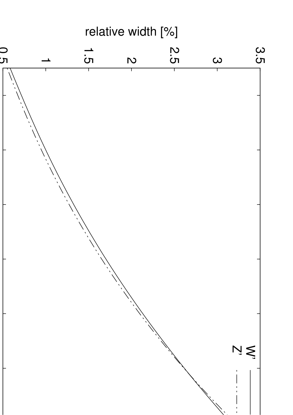
Therefore, the only decay channel for the $W^{\prime}$ in the ideally delocalized scenario is the decay into a $W$ and a $Z$. The $Z^{\prime}$ can in principle also decay into SM fermions; however, the decay of the longitudinal mode enhances the $WZ$ decay channel by a factor of

$$\frac{m_{Z^{\prime}}^{4}}{16m_{W}^{2}m_{Z}^{2}}$$

over the decay into a fermion pair causing the latter decay to be highly suppressed by a factor of the order of $\mathcal{O}(10^{-2})$ (cf. [6]). Looking at figure 2 we find that the resonances are rather narrow ($\Gamma_{V}/m_{V}\approx 1-3\%$) improving the prospects for observing these particles at the LHC.

The new heavy fermions decay into their light partner and a gauge boson, the resulting widths being of the order $\Gamma_{f}/m_{f}\approx 0.1$, which, combined with their large mass ($>2\,\mathrm{TeV}$), will make the direct detection as a resonance at a collider rather challenging.

For a massless SM fermion, the Yukawa coupling between the sites $1$ and $2$ vanishes. From $\mathcal{L}_{\text{Yukawa}}$ we find that the wave function is completely fixed by the delocalization parameter $\epsilon_{L}$. Therefore, the influence of $m_{\text{bulk}}$ on the wave functions of the light SM fermions and their couplings is very small and the dependence of the cross section on $m_{\text{bulk}}$ is almost negligible at LHC energies.

Although ideal delocalization guarantees compatibility with the constraints from EWPT at tree level [5], a recent 1-loop analysis [7] has shown that a deviation from ideal delocalization is necessary to comply with the EWPT constraints at loop level. According to the authors of [7], this deviation corresponds to an on-shell coupling between the $W^{\prime}$ and the light fermions as large as $1-2\%$ of the isospin gauge coupling $g_{W}\approx g_{0}$.

The coupling $g_{W^{\prime}ff}$ to which the bounds derived in [7] apply is defined in the effective theory obtained by integrating out the bulk fermions and is renormalized at the $W^{\prime}$ mass shell. There are two operators contributing to this coupling in the one loop analysis in addition to the coupling of the left-handed fermions to the component of the $W^{\prime}$ sitting at site $0$. The first one

$$O_{1}=\overline{\Psi}_{0,L}\Sigma_{0}\mathchoice{\vtop{\halign{#\cr$\hfil\displaystyle\mkern 0.0mu/\hfil$\crcr$\displaystyle A_{1}$\crcr}}}{\vtop{\halign{#\cr$\hfil\textstyle\mkern 0.0mu/\hfil$\crcr$\textstyle A_{1}$\crcr}}}{\vtop{\halign{#\cr$\hfil\scriptstyle\mkern 0.0mu/\hfil$\crcr$\scriptstyle A_{1}$\crcr}}}{\vtop{\halign{#\cr$\hfil\scriptscriptstyle\mkern 0.0mu/\hfil$\crcr$\scriptscriptstyle A_{1}$\crcr}}}\Sigma_{0}^{\dagger}\Psi_{0,L}$$

(2)

encodes a coupling between the component of the $W^{\prime}$ sitting at site $1$ and the left-handed SM fermion and is generated by integrating out the bulk fermion from the diagram in figure 3 (see also [4]). The second operator

$$O_{2}=\overline{\Psi}_{0,L}\left(D_{\nu}\left(\Sigma_{0}F_{1}^{\mu\nu}\Sigma_{0}^{\dagger}\right)\right)\gamma_{\mu}\Psi_{0,L}$$

(3)

arises from loop corrections. Although this operator also contains a contribution to the coupling between the left-handed fermion and the gauge bosons at site $1$, it has a nontrivial momentum structure. However, using a non-linear field redefinition in the spirit of on-shell effective field theory [9], the corresponding part of $O_{2}$ can be converted to the same form as $O_{1}$ at the price of introducing additional higher dimensional operators coupling at least two gauge bosons to two fermions whose contributions are suppressed by another power of the gauge couplings. This allows the operator $O_{2}$ to be included into $g_{W^{\prime}ff}$ where it contributes to the bounds derived by the authors of [7].

Therefore, the contributions of both these operators can be accounted for by adjusting the delocalization parameter $\epsilon_{L}$ in the tree level Lagrangian $\mathcal{L}_{\text{Yukawa}}$ to generate the coupling $g_{W^{\prime}ff}$. The model parameters then should be understood to be renormalized at the $W^{\prime}$ mass.

In the case of light SM fermions and their partners, only the wave functions of the left-handed fermions depend on the delocalization parameter $\epsilon_{L}$. Therefore, the right-handed couplings between the new gauge bosons and the light SM fermions are not affected by the departure from ideal delocalization. Denoting the wave functions by $\phi_{f,L,i}$ and $\phi_{Z^{\prime},i}$ and using the normalization of the fermion wave functions, the left-handed coupling of a fermion to the $Z^{\prime}$ can be written as

$$\sum_{i=0}^{1}\phi_{f,L,i}^{2}\left(\pm\frac{1}{2}g_{i}\phi_{Z^{\prime},i}+Yg_{2}\phi_{Z^{\prime},2}\right)=\pm\frac{1}{2}\sum_{i=0}^{1}g_{i}\phi_{Z^{\prime},i}\phi_{f,L,i}^{2}+Yg_{2}\phi_{Z^{\prime},2}\,,$$

(4)

with the sign depending on the isospin of the fermion and $Y$ denoting the hypercharge. As tuning away from ideal delocalization shifts the light mode of the fermion towards the heavy $Z^{\prime}$ sitting at site $1$, the isospin dependent part in (4) grows, while the correction to $g_{Z^{\prime}uu}$ differs only in sign from the correction to $g_{Z^{\prime}dd}$.

Figure 4 shows the dependence of $g_{W^{\prime}ff}$, $g_{Z^{\prime}dd}$ and $g_{Z^{\prime}uu}$ on the delocalization parameter and clearly demonstrates this behavior. Considering that we have both $u\bar{u}$ and $d\bar{d}$ initial states at the LHC, that both couplings start with positive values of the same order of magnitude at the point of ideal delocalization and that we also have right-handed couplings of the same order of magnitude which don’t depend on $\epsilon_{L}$ at all, we don’t expect a large impact from changing $\epsilon_{L}$ on $Z^{\prime}$ production in the $s$-channel. On the other hand, the effect on the $s$-channel $W^{\prime}$ production should be sizable, because $\epsilon_{L}$ interpolates between this channel being forbidden and being about the same order of magnitude as $Z^{\prime}$ production.

Figure 5 shows the same plot as figure 4 for the other regions of parameter space probed in our Monte Carlo simulations. In all three plots, changing $m_{\text{bulk}}$ doesn’t generate a visible change of the actual couplings, but does move the gray band of acceptable $g_{W^{\prime}ff}$ values.

We have coded a FORTRAN 90 module which diagonalizes the lagrangian of the model and calculates all masses and couplings. Furthermore, the module calculates the tree level widths of all new particles. Non ideal delocalization is implemented by tuning the parameter $\epsilon_{L}$ away from the value required for vanishing $g_{W^{\prime}ff}$. For the automatized generation of tree level matrix elements, we encoded the model in unitarity gauge into the optimizing matrix element generator O’Mega [10, 11] which is part of the Monte Carlo eventgenerator generator WHIZARD [11]. The results presented below are based on Monte Carlo simulations using WHIZARD [11].

We checked the couplings calculated by our FORTRAN code against all the couplings for which analytic expressions are given in [4]. To check the validity of our implementation of the model, we compared the cross sections for a number of $2\rightarrow 2$ processes to the SM, taking $m_{W^{\prime}}$, $m_{\text{bulk}}$ and $m_{\text{Higgs}}$ to be huge. The widths calculated by the FORTRAN module using analytic formulae were checked against numeric results obtained from amplitudes generated by O’Mega.

We also checked gauge invariance by numerically checking the Ward Identities in the model obtained by taking the limit

$$\sqrt{2}v=\left<\Sigma_{0/1}\right>\rightarrow 0\,,$$

where the exact $\mathbf{SU}(2)_{0}\times\mathbf{SU}(2)_{1}\times\mathbf{U}(1)_{2}$ gauge symmetry is restored.

In addition, we compared several $2\rightarrow 2$ cross sections to the CalcHep [12] implementation of the model used by the authors of [6]. After plugging in the correct $W^{\prime}$ and $Z^{\prime}$ widths, the results turn out to be in perfect agreement.

In the ideally delocalized scenario, only the $Z^{\prime}$ has nonvanishing tree level couplings to the SM fermions, while the $W^{\prime}$ is perfectly fermiophobic. As explained above, the $Z^{\prime}$ decays with a branching ratio of over $95\%$ into a $W^{+}W^{-}$ pair, rendering the resulting four fermion final state highly favored over the two lepton one. This is in sharp contrast to many new heavy neutral gauge bosons predicted by other extensions of the SM (Little Higgs, GUTs etc.) which usually have larger fermion couplings but small or vanishing couplings to the SM gauge bosons, because they typically originate from different gauge group factors and have little or no mixing with the SM gauge bosons [13, 14].

The most interesting final states for $Z^{\prime}$ production are thus $jjjj$, $l\nu jj$ and $l\nu l\nu$. The four jet final state however is highly contaminated from backgrounds containing gluon jets, and the two neutrino final state suffers from the momentum information missing for the two neutrinos, leaving $l\nu jj$ as the most promising candidate assuming one can cope with the missing neutrino momentum.

Figure 6 shows a representative of the class of diagrams contributing to the signal in this process. In addition to the signal, there are also reducible backgrounds from events with neutral jet pairs and an irreducible background from diagrams not of the type figure 6 contributing to the same final state. In this and the next section, we assume that a veto on forward tagging jets is effective in suppressing the background from vector boson fusion.

For the construction of an observable that can deal with the missing longitudinal neutrino momentum, consider the decay of an on-shell $W$ into a lepton with momentum $p_{l}=q$ and a neutrino with momentum $p_{\nu}=p$. The mass shell conditions of neutrino and $W$ boson then give two equations involving the neutrino energy $p_{0}$ and longitudinal momentum $p_{L}$

	$\displaystyle p_{0}^{2}-p_{L}^{2}-\left|\vec{p}_{\perp}\right|^{2}$	$\displaystyle=0$		(5a)
	$\displaystyle p_{0}q_{0}-p_{L}q_{L}-\vec{p}_{\perp}\vec{q}_{\perp}$	$\displaystyle=\frac{m_{W}^{2}}{2}$		(5b)

(assuming the lepton to be massless), with $\vec{p}_{\perp}$ and $\vec{q}_{\perp}$ the projections of the momenta onto the transverse plane. (5a) describes a hyperbola in the $p_{L}-p_{0}$ plane and (5b) describes a straight line with the modulus of the slope smaller than $1$. These curves are parametrized by $\vec{p}_{\perp}$, $q$ and $m_{W}$ and one of their (two in general) intersections gives the neutrino energy and longitudinal momentum as a function of these quantities. This geometrical situation is depicted in figure 7.

This construction allows us to reconstruct the full neutrino momentum from the lepton momentum and the missing $p_{T}$ for the events coming from the decay of a quasi-on-shell $W$. However, owing to the modulus of the slope of the straight line being smaller than one, we always have two solutions, none of which is preferred on kinematical grounds. We have elected to deal with this by counting both solutions in the histograms, effectively doubling the amount of background events while preserving the size of the signal. The two points of intersection can be obtained analytically by

$$p_{0}=\frac{q_{0}^{2}\left(m_{W}^{2}+2\vec{p}_{\perp}\vec{q}_{\perp}\right)\pm q_{L}A}{2q_{0}\left(q_{0}^{2}-q_{L}^{2}\right)}\quad,\quad p_{L}=\frac{q_{L}\left(m_{W}^{2}+2\vec{p}_{\perp}\vec{q}_{\perp}\right)\pm A}{2\left(q_{0}^{2}-q_{L}^{2}\right)}\,,$$

(6)

with the abbreviation

$$A=q_{0}\sqrt{\left(m_{W}^{2}+2\vec{p}_{\perp}\vec{q}_{\perp}\right)^{2}+4\vec{p}_{\perp}^{2}\left(q_{L}^{2}-q_{0}^{2}\right)}\,.$$

To investigate the possibility of discovering the $Z^{\prime}$ in $pp\rightarrow jjl+p_{T,\text{miss}}$ at the LHC we have performed full parton-level Monte Carlo simulations for an integrated luminosity of $\int\mathcal{L}=100\,\mathrm{fb^{-1}}$, the lepton being either an electron or a muon and each jet being either a quark (excluding the top) or a gluon. To suppress the backgrounds, we have applied $p_{T}$-cuts to all visible particles and to $p_{T,\text{miss}}$

$$p_{T}\geq 50\,\mathrm{GeV}\,.$$

In addition, we have required the polar and intermediary angles of all visible particles to lie within

$$-0.95\leq\cos\theta\leq 0.95$$

and also applied a small-$x$ cut to the ingoing partons

$$x\geq 1.4\cdot 10^{-3}$$

to avoid infrared singularities in the amplitude. For identifying the intermediary $W$ we applied a cut to the invariant mass of the two jets¹¹ 1 See section 7 for a discussion of the effects of finite jet resolution on the identification of the $W$.

$$75\,\mathrm{GeV}\leq m_{jj}\leq 85\,\mathrm{GeV}\,.$$

We used (6) to reconstruct the neutrino momentum, counting both solutions into the histograms and discarding those with negative neutrino energy.

The plot on the left of figure 8 compares the invariant mass distribution obtained from the reconstructed neutrino momenta to that obtained from the unobservable neutrino momenta taken from Monte Carlo data for $m_{W^{\prime}}=500\,\mathrm{GeV}$ and $m_{\text{bulk}}=3.5\,\mathrm{TeV}$. In both cases the peak from the $Z^{\prime}$ is clearly visible. As expected, counting both solutions obtained from the reconstruction doubles the amount of background events while the number of events contained in the peak stays roughly the same. However, the peak is broadened by the reconstruction, which can been seen when comparing to a SM simulation (dotted line). The broadening at the center of the peak is mainly caused by the mismatch between reconstructed and true neutrino momentum of the signal events due to the $W$ not being exactly on-shell; the sidebands of the peak are caused by the second solutions for $p_{\nu}$ of events at the center of the peak.

The plot on the right of figure 8 shows the effect of changing the delocalization parameter $\epsilon_{L}$ in the range allowed by the EWPT at one loop (cf. section 3), again for $m_{W^{\prime}}=500\,\mathrm{GeV}$ and $m_{\text{bulk}}=3.5\,\mathrm{TeV}$. As argued before, the impact on the invariant mass distribution is not strong, the peak staying clearly visible over the whole range of allowed values of $\epsilon_{L}$.

Figure 9 shows the invariant mass distributions obtained for

$$m_{W^{\prime}}\in\left\{380\,\mathrm{GeV},500\,\mathrm{GeV},600\,\mathrm{GeV}\right\}\,,$$

which covers the whole range of values allowed by the EWPT at one loop²² 2 We also changed $m_{\text{bulk}}$ as shown in figure 9 to comply with the EWPT; however, as explained in section 3, this has no noticeable effect on the cross section. [4, 7]. As the masses of the $Z^{\prime}$ and $W^{\prime}$ are quasi-degenerate, the $Z^{\prime}$ peak moves with changing $m_{W^{\prime}}$. The histogram shows that the peak stays clearly observable, although it decreases in size as $m_{W^{\prime}}$ becomes larger owing to the smaller parton distribution functions for the sea quarks at larger values of $x$.

To get a quantitative handle on the significance of the signal and to estimate the minimal luminosity necessary for discovering the $Z^{\prime}$, we define the raw signal $N$ to be the number of events in the $\pm 20\,\mathrm{GeV}$ region around the peak. To estimate the background we have generated SM events for an integrated luminosity of $\int\mathcal{L}=400\,\mathrm{fb^{-1}}$, analyzed this data the in the same way as the Monte Carlo data for the three site model and then downscaled the resulting distributions by a factor of $4$ to reduce the error coming from fluctuations in the background. We denote the number of background events in the $\pm 20\,\mathrm{GeV}$ region around the peak obtained this way by $N_{b}$.

We define the signal $N_{s}$ as

$$N_{s}=N-N_{b}\,.$$

(7)

The number of background events in the original Monte Carlo data $N^{\prime}_{b}$ is roughly doubled by our momentum reconstruction

$$N_{b}=2N^{\prime}_{b}$$

and the standard deviation of $\sigma_{N_{b}}$ of $N_{b}$ must scale accordingly, resulting in

$$\sigma_{N_{b}}=2\sigma_{N^{\prime}_{b}}=2\sqrt{N^{\prime}_{b}}=\sqrt{2N_{b}}\,.$$

We then define the significance in the usual way:

$$s=\frac{N_{s}}{\sigma_{N_{b}}}=\frac{N-N_{b}}{\sqrt{2N_{b}}}\,.$$

(8)

The significance of the signal in the ideally delocalized scenario thus calculated is shown in figure 10 together with the $5\sigma$ and $3\sigma$ discovery thresholds. The $5\sigma$ thresholds are approx. $1\,\mathrm{fb^{-1}}$, $2\,\mathrm{fb^{-1}}$, $5\,\mathrm{fb^{-1}}$ for $m_{W^{\prime}}=380\,\mathrm{GeV}$, $500\,\mathrm{GeV}$, $600\,\mathrm{GeV}$, respectively. Considering the fact that tuning $\epsilon_{L}$ into the region allowed by the EWPT does not significantly change the signal, the three-site $Z^{\prime}$ may be discovered as early as in the first $1-2\,\mathrm{fb^{-1}}$ and even in the worst case can be expected to manifest itself in the first $10-20\,\mathrm{fb^{-1}}$ of data.

As discussed in section 3, the deviation from ideal delocalization required by the EWPT at one loop leads to non-vanishing couplings of the $W^{\prime}$ to the SM fermions of the same order of magnitude as the $Z^{\prime}ff$ couplings. This allows for the possibility of producing the $W^{\prime}$ in the $s$-channel at the LHC.

There are two possible decay channels for the $W^{\prime}$ that are promising candidates for discovering this resonance. The first possibility is the decay $W^{\prime}\rightarrow WZ\rightarrow l\nu_{l}jj$ (cf. the left plot in figure 11), which is the final state already discussed in the last section and which can be treated the same way (replacing the cut on the $W$ mass with a cut on the $Z$ mass). The second possibility is the decay of the $ZW$ pair into two leptons and two jets (cf. the right plot in figure 11). The absence of missing $p_{T}$ is a clear advantage of this decay mode allowing for background suppression by cutting on the invariant mass of the lepton pair; unfortunately, the branching ratio is smaller than that for the $l\nu_{l}jj$ mode.

To probe the $l\nu_{l}jj$ final state we have used the same Monte Carlo data and cuts as in section 5 replacing the cut on the invariant mass³³ 3 See section 7 for a discussion of the effects of finite jet resolution on the separation of $W$ and $Z$. of the jet pair with

$$86\,\mathrm{GeV}\leq m_{jj}\leq 96\,\mathrm{GeV}\,.$$

For probing the $lljj$ final state we again performed Monte Carlo simulations for an integrated luminosity of $\int\mathcal{L}=100\,\mathrm{fb^{-1}}$. We applied the same $p_{T}$, $x$ and angular cuts as in the last section together with the identification cuts

$$75\,\mathrm{GeV}\leq m_{jj}\leq 85\,\mathrm{GeV}\quad,\quad 86\,\mathrm{GeV}\leq m_{ll}\leq 96\,\mathrm{GeV}$$

(9)

on the invariant mass of the jet pair and on that of the dilepton system.

Figure 12 shows the invariant mass distributions obtained for both final states for $m_{W^{\prime}}=380\,\mathrm{GeV}$, $500\,\mathrm{GeV}$, $600\,\mathrm{GeV}$ and $\epsilon_{L}$ chosen from the allowed range such as to give large values⁴⁴ 4 Even larger values of $g_{W^{\prime}ff}$ are allowed by increasing $m_{\text{bulk}}$, but we are more interested in the lowest possible value for which the $W^{\prime}$ might still be detected in this channel at the LHC. of $g_{W^{\prime}ff}$ (cf. figures 4 and 5). For both final states, the resonance peaks can be clearly seen for all three values of $m_{W^{\prime}}$. The total number of events for $lljj$ is much smaller compared to $l\nu_{l}jj$ owing to the smaller branching ratio, but the cuts on both $m_{Z}$ and $m_{W}$ and the absence of the double counting introduced by the neutrino reconstruction significantly improve the signal to background ratio.

The dependence of the resonance peak on the delocalization parameter $\epsilon_{L}$ is shown in figure 13. The left column shows the $\pm 50\,\mathrm{GeV}$ region around the peak for the $l\nu_{l}jj$ final state for different values of $\epsilon_{L}$ and for the case of ideal delocalization. For $m_{W^{\prime}}=500\,\mathrm{GeV}$ and $m_{W^{\prime}}=600\,\mathrm{GeV}$ the peak vanishes in the case of ideal delocalization which demonstrates that the cut (9) is sufficient to discriminate between jets coming from the decay of $W$ and those coming from a $Z$. In the case of $m_{W^{\prime}}=380\,\mathrm{GeV}$, a small peak remains even in the case of ideal delocalization which stems from jets coming from $pp\rightarrow Z^{\prime}\rightarrow l\nu_{l}jj$ misidentified as a $Z$ (we will discuss the possibility of unfolding these two contribution in the next section).

The histograms show that tuning $\epsilon_{L}$ towards the point of ideal delocalization quickly decreases the size of the peak making it invisible for the lowest chosen values of $\epsilon_{L}$. The right column shows the same region around the peak for the final state $lljj$ and the same values of $\epsilon_{L}$. As should be expected, the same decrease of the peak size is visible.

To obtain a numerical estimate for the integrated luminosity required for a $s=5\sigma$ or $3\sigma$ discovery of the $W^{\prime}$ at some given value of the delocalization parameter $\epsilon_{L}$ we exploit the fact that the significance of the signal scales as $g_{W^{\prime}ff}^{2}$ with the coupling of $W^{\prime}$ to left-handed SM fermions. This allows us to estimate the integrated luminosity required for obtaining a signal with significance $s_{0}$ in terms of the significance of the signal for other values of coupling and integrated luminosity.

For the actual determination of $s$ from Monte Carlo data we define the signal as in section 5. In case of the $l\nu_{l}jj$ final state we calculate $s$ via (8), while for the case of $lljj$ it can be calculated simply as

$$s=\frac{N_{s}}{\sqrt{N_{b}}}\,,$$

(10)

because we don’t have the additional doubling of the background events by the neutrino momentum reconstruction in this case⁵⁵ 5 Because of the lower number of events in the final state $lljj$, the background for this case was calculated for an integrated luminosity of $\int\mathcal{L}=1000\,\mathrm{fb^{-1}}$ and scaled down..

The significances calculated this way at different points in parameter space are shown in table 1. For $m_{W^{\prime}}=380\,\mathrm{GeV}$ and $m_{W^{\prime}}=500\,\mathrm{GeV}$, both final states seem to do equally well at revealing the fermionic couplings of the $W^{\prime}$; however, for $m_{W^{\prime}}=600\,\mathrm{GeV}$ the dilepton final state appears to give a slightly better signal owing to the better ratio of signal to background.

The integrated luminosity necessary for a $5\sigma$ resp. $3\sigma$ discovery of the $W^{\prime}$ in the $s$-channel is shown in figure 14 together with the range of the delocalization parameter $\epsilon_{L}$ allowed for the different choices of $m_{W^{\prime}}$ and $m_{\text{bulk}}$. Taking the integrated luminosity collected over the full LHC running time to be around $400\,\mathrm{fb^{-1}}$ and considering the fact that the band of allowed $\epsilon_{L}$ (and $g_{W^{\prime}ff}$) can be moved further towards smaller values by lowering $m_{\text{bulk}}$, it is evident from figure 14 that there is a part of the allowed parameter space in which the $W^{\prime}$ would appear perfectly fermiophobic at the LHC. However, there also is a big region of parameter space in which the coupling of the $W^{\prime}$ to the SM fermions eventually should be discovered, although this still would take several years of running time as the lowest integrated luminosity required for $3\sigma$ is around $10\,\mathrm{fb^{-1}}$ even at the point in parameter space most easily accessible.

Since flavor tagging is impossible for light quark flavors, we have to rely on invariant mass cuts for the jet pairs to be able to separate the case of the two jets in $l\nu_{l}jj$ coming from the decay of a $W$ in $Z^{\prime}$ production from that of the jets being produced by a decaying $Z$ in $W^{\prime}$ production. However, it may very well be impossible to obtain a resolution of order $\pm 5\,\mathrm{GeV}$ in the jet invariant mass from experimental data. In this section, we discuss the effect of a gaussian smearing of the invariant mass of the jets on our analysis.

In the ideal case of exact $m_{jj}$ measurement, events coming from the decay of a intermediary $W$/$Z$ are distributed according to a Breit-Wigner distribution

$$p_{b}(x,m,\Gamma)\>dx=\frac{n_{b}(m,\Gamma)^{-1}}{\left(x^{2}-m^{2}\right)^{2}+\Gamma^{2}m^{2}}\>dx\,,$$

with the normalization factor

$$n_{b}(m,\Gamma)=\frac{\pi}{4m^{3}}\left(1+\frac{\Gamma^{2}}{m^{2}}\right)^{-\frac{3}{4}}\sin^{-1}\left(\frac{1}{2}\atan\frac{\Gamma}{m}\right)\,.$$

Emulating the measurement error in the jet mass by convoluting $p_{\text{bw}}$ with a gaussian of standard deviation $\sigma$

$$p_{\text{g}}(x,\sigma)\>dx=\frac{1}{\sqrt{2\pi}\sigma}e^{-\frac{x^{2}}{2\sigma^{2}}}\>dx$$

we obtain the smeared distribution

$$p_{\text{sm}}(x,m,\Gamma,\sigma)\>dx=\int_{0}^{\infty}dy\>p_{b}(y,m,\Gamma)p_{\text{g}}(x-y,\sigma)\,.$$

Figure 15 shows the effect of this smearing on the Breit-Wigner peaks of the $Z$ and the $W$. Turning on the smearing and increasing $\sigma$ causes the sharp Breit-Wigner peaks to decay rapidly, and for $\sigma=10\,\mathrm{GeV}$, only two very broad bumps are left. The result is that, if a cross section has one contribution which stems from the decays of a virtual $Z$ and one coming from a virtual $W$, any attempt to isolate the $Z$ contribution by cutting on the resonance will inevitably also select events coming from the $W$ decay contaminating the sample (and vice versa). Therefore, our analysis of the $l\nu_{l}jj$ final state will show a $W^{\prime}$ peak even in the case of ideal delocalization which is caused by jet pairs from a decaying $W$ misidentified as a $Z$.

If we try to isolate the $W$ peak with a cut on the invariant mass $m_{jj}$

$$L_{W}\leq m_{jj}\leq U_{W}$$

and the $Z$ peak with a cut

$$L_{Z}\leq m_{jj}\leq U_{Z}\,,$$

then the resulting event counts $\widetilde{N}_{W},\widetilde{N}_{Z}$ can be calculated from the true event counts $N_{W},N_{Z}$ coming from a decaying $W$ or $Z$ via a matrix $T$ as

$$\begin{pmatrix}\widetilde{N}_{W}\\ \widetilde{N}_{Z}\end{pmatrix}=\begin{pmatrix}T_{WW}&T_{WZ}\\ T_{ZW}&T_{ZZ}\end{pmatrix}\begin{pmatrix}N_{W}\\ N_{Z}\end{pmatrix}$$

with entries

$$T_{ij}=\int_{L_{i}}^{U_{i}}dm\>p_{\text{sm}}(m,m_{j},\Gamma_{j},\sigma)\,.$$

Inverting $T$ we can calculate the event counts $N_{W}$ and $N_{Z}$

$$\begin{pmatrix}N_{W}\\ N_{Z}\end{pmatrix}=T^{-1}\begin{pmatrix}\widetilde{N}_{W}\\ \widetilde{N}_{Z}\end{pmatrix}\,.$$

(11)

The entries of $T$ give the probability of misidentifying an event and can be readily calculated numerically; for example, choosing cuts

$$L_{W}=60\,\mathrm{GeV}\quad,\quad U_{W}=85\,\mathrm{GeV}\quad,\quad L_{Z}=86\,\mathrm{GeV}\quad,\quad U_{Z}=111\,\mathrm{GeV}$$

yields

$$T\approx\begin{pmatrix}0.64&0.27\\ 0.29&0.62\end{pmatrix}\quad,\quad T^{-1}\approx\begin{pmatrix}1.9&-0.85\\ -0.89&2.0\end{pmatrix}\,.$$

This way, we can in principle use $T$ to disentangle the contributions from $W$ and $Z$ resonances to the signal in the presence of a measurement error which causes the Breit-Wigner peaks to lose their shape. However, to apply this to actual data, it is vital to separate the signal from both the reducible and the irreducible backgrounds, because they don’t follow a Breit-Wigner distribution.

In order to estimate the significance of a signal obtained this way, we calculate the standard deviation $\sigma_{N_{i}}$ of $N_{i}$ according to

$$\sigma_{N_{i}}=\sqrt{\sum_{j\in W,Z}\left(T^{-1}_{ij}\right)^{2}\sigma_{\widetilde{N}_{j}}^{2}}\,.$$

In our analysis, we obtain the signal events inside the smeared Breit-Wigner peaks $\widetilde{N}_{i}$ by subtracting the background $N_{b,i}$ from the total number of events $N_{t,i}$. The error on $N_{t,i}$ is

$$\sigma_{N_{t,i}}=\sqrt{N_{i}+2N_{b,i}}=\sqrt{N_{t,i}+N_{b,i}}\,,$$

because of the neutrino momentum reconstruction doubling the amount of background events (cf. section 5), and we finally arrive at

$$\sigma_{N_{i}}=\sqrt{\sum_{j\in W,Z}\left(T^{-1}_{ij}\right)^{2}\left(N_{t,j}+N_{b,j}\right)}$$

(12)

For a simulation of the effect of the measurement error our analysis we have randomly distributed the invariant mass of the jet pairs within a gaussian with width $\sigma=10\,\mathrm{GeV}$ centered around the correct value calculated from Monte Carlo data. We then did the same analysis as in sections 5 and 6 with $m_{W^{\prime}}=500\,\mathrm{GeV}$ and $m_{\text{bulk}}=3.5\,\mathrm{TeV}$ both for $\epsilon_{L}=0.254$ and for the ideally delocalized scenario. The only difference to the previous analysis are the cuts on $m_{jj}$ which we enlarged to

$$60\,\mathrm{GeV}\leq m_{jj}\leq 85\,\mathrm{GeV}\quad\text{resp.}\quad 86\,\mathrm{GeV}\leq m_{jj}\leq 111\,\mathrm{GeV}\,.$$

Figure 16 shows the resulting effect on the $W^{\prime}$ peak for the cases of ideal delocalization (left) and for $\epsilon_{L}=0.254$ (right). In both cases a peak is clearly visible, which in the ideally delocalized scenario is only composed of events with jets coming from a decaying $W$ misidentified as a $Z$.

The number of signal events $\widetilde{N}_{W/Z}$ after smearing, the significance $s_{W/Z}$ of these calculated via (8), $N_{W/Z}$ obtained from applying the transfer matrix $T^{-1}$ (11) and the resulting significance $N_{i}/\sigma_{N_{i}}$ obtained from (12) are shown in table 2. All peaks are significant with $s>5\sigma$; however, after applying the transfer matrix, the $W^{\prime}$ peak vanishes within one standard deviation for ideal delocalization, while in the case of $\epsilon_{L}=0.254$ a residue as big as $2\sigma$ remains. The $Z^{\prime}$ peak remains significant after applying the transfer matrix, however, the significance is reduced because the transfer matrix enlarges the error.

What are the consequences for the detection of $Z^{\prime}$ and $W^{\prime}$ in the $l\nu_{l}jj$ final state? The detection of the $Z^{\prime}$ is not affected by inaccuracies in the jet mass resolution as the peak is always present with little variations of its size over the whole parameter space, and we can always compensate for the smearing of the jet mass by enlarging the cut window on $m_{jj}$. However, the separation of a possible $W^{\prime}$ contribution to the peak (which depends heavily on the point in parameter space) by cutting on $m_{jj}$ alone is spoiled by the error in $m_{jj}$; we have to apply additional tricks like the transfer matrix (11) to disentangle the two contributions. While this seems to work in principle, the significance of the $W^{\prime}$ signal is reduced by this analysis, rendering this final state much less suitable for detecting a coupling between $W^{\prime}$ and SM fermions than the decay into $lljj$ which is not contaminated by a contribution of the $Z^{\prime}$.

We have studied the production of the heavy $W^{\prime}$ and $Z^{\prime}$ bosons of the three site higgsless model in the $s$-channel at the LHC. Unlike vector boson fusion, this production mode allows to directly measure the couplings of the new bosons to standard model fermions. These couplings are constrained by electroweak precision tests and their measurement is therefore crucial for consistency checks of models of electroweak symmetry breaking with extended gauge sectors.

We have found a method that will allow the separation of $W^{\prime}$ from $Z^{\prime}$ processes at the parton level. Our results show that the observation of $s$-channel production of $Z^{\prime}$ bosons will not require a lot of integrated luminosity for all of the allowed parameter space. In contrast, $W^{\prime}$ production in the $s$-channel is much more sensitive to the model parameters and there are regions of parameter space where an observation will be very challenging, if not impossible. A more detailed experimental analysis should investigate the effects of hadronization and detector response on our results.

This research is supported by Deutsche Forschungsgemeinschaft through the Research Training Group 1147 Theoretical Astrophysics and Particle Physics, by Bundesministerium für Bildung und Forschung Germany, grant 05HT6WWA and by the Helmholtz Alliance Physics at the Terascale.

References

- [1] L. Randall and R. Sundrum, Phys. Rev. Lett. 83, 3370 (1999), [arXiv:hep-ph/9905221].
- [2] J. M. Maldacena, Adv. Theor. Math. Phys. 2, 231 (1998), [Int. J. Theor. Phys. 38, 1113 (1999)], [arXiv:hep-th/9711200].
- [3] N. Arkani-Hamed, A. G. Cohen and H. Georgi, Phys. Rev. Lett. 86, 4757 (2001) [arXiv:hep-th/0104005].
- [4] R. S. Chivukula et al., Phys. Rev. D74, 075011 (2006) [arXiv:hep-ph/0607124].
- [5] R. S. Chivukula, E. H. Simmons, H. J. He, M. Kurachi and M. Tanabashi, Phys. Rev. D72, 015008 (2005) [arXiv:hep-ph/0504114].
- [6] H. J. He et al., Phys. Rev. D78, 031701 (2008). [arXiv:0708.2588 [hep-ph]].
- [7] T. Abe, S. Matsuzaki and M. Tanabashi, [arXiv:0807.2298 [hep-ph]].
- [8] R. Casalbuoni, S. De Curtis, D. Dominici and R. Gatto, Phys. Lett. B155, 95 (1985).
- [9] H. Georgi, Nucl. Phys. B361, 339 (1991).
- [10] M. Moretti, T. Ohl and J. Reuter, [arXiv:hep-ph/0102195].
- [11] W. Kilian, T. Ohl and J. Reuter, [arXiv:0708.4233 [hep-ph]].
- [12] A. Pukhov, [arXiv:hep-ph/0412191].
- [13] T. G. Rizzo, [arXiv:hep-ph/0610104].
- [14] P. Langacker, [arXiv:0801.1345 [hep-ph]].