A Spectral Method for Elliptic Equations:
The Dirichlet Problem

Kendall Atkinson Affiliation: Departments of Mathematics & Computer Science Affiliation: The University of Iowa David Chien Olaf Hansen Affiliation: Department of Mathematics Affiliation: California State University San Marcos

Abstract

Let $\Omega$ be an open, simply connected, and bounded region in $\mathbb{R}^{d}$ , $d\geq 2$ , and assume its boundary $\partial\Omega$ is smooth. Consider solving an elliptic partial differential equation $Lu=f$ over $\Omega$ with zero Dirichlet boundary values. The problem is converted to an equivalent elliptic problem over the unit ball $B$ , and then a spectral method is given that uses a special polynomial basis. With sufficiently smooth problem parameters, the method is shown to have very fast convergence. Numerical examples illustrate exponential convergence.

1 INTRODUCTION

Consider solving the elliptic partial differential equation

Lu(\mathbf{s})\equiv-\sum_{i,j=1}^{d}\frac{\partial}{\partial s_{i}}\left(a_{i,j}(\mathbf{s})\frac{\partial u(\mathbf{s})}{\partial s_{j}}\right)+\gamma(\mathbf{s})u(\mathbf{s})=f(\mathbf{s}),\quad\quad\mathbf{s}\in\text{$\Omega$}\subseteq\mathbb{R}^{d}

(1)

with the Dirichlet boundary condition

u(\mathbf{s})\equiv 0,\quad\quad\mathbf{s}\in\partial\Omega

(2)

Assume $d\geq 2$ . Assume $\Omega$ is an open, simply-connected, and bounded region in $\mathbb{R}^{d}$ , and assume that its boundary $\partial\Omega$ is several times continuously differentiable. Similarly, assume the functions $\gamma(\mathbf{s}),$ $f(\mathbf{s}),$ $a_{i,j}(\mathbf{s})$ are several times continuously differentiable over $\overline{\Omega}$ . As usual, assume the matrix $A(\mathbf{s})=\left[a_{i,j}(\mathbf{s})\right]$ is symmetric, and also assume it satisfies the strong ellipticity condition,

\xi^{\text{T}}A(\mathbf{s})\xi\geq c_{0}\xi^{\text{T}}\xi,\quad\quad\mathbf{s}\in\overline{\Omega},\quad\xi\in\mathbb{R}^{d}

(3)

with $c_{0}>0$ . Also assume $\gamma(\mathbf{s})\geq 0$ , $\mathbf{s}\in\Omega$ .

In §2 we consider the special region $\Omega=B$ , the open unit ball in $\mathbb{R}^{d}$ . We define a Galerkin method for (1)-(2) with a special finite-dimensional subspace of polynomials, and we give an error analysis that shows rapid convergence of the method. In §3 we discuss the use of a transformation from a general region $\Omega$ to the unit ball $B$ , showing that the transformed equation is again elliptic over $B$ . Implementation issues are discussed in §4 for problems in $\mathbb{R}^{2}$ and $\mathbb{R}^{3}$ . We conclude in §5 with numerical examples in $\mathbb{R}^{2}$ and $\mathbb{R}^{3}$ .

The methods of this paper generalize to the equation

	$\displaystyle Lu(\mathbf{s})\equiv$	$\displaystyle-\sum_{i,j=1}^{d}\frac{\partial}{\partial s_{i}}\left(a_{i,j}(\mathbf{s})\frac{\partial u(\mathbf{s})}{\partial s_{j}}\right)$
		$\displaystyle+\sum_{j=1}^{d}b_{j}\left(\mathbf{s}\right)\frac{\partial u(\mathbf{s})}{\partial s_{j}}+\gamma(\mathbf{s})u(\mathbf{s})=f(\mathbf{s}),\quad\quad\mathbf{s}\in\text{$\Omega$}\subseteq\mathbb{R}^{d}$

which contains first order derivative terms, provided the operator $L$ is strongly elliptic. To do so, use the results of Brenner and Scott [5, §§2.6-2.8], combined with the methods of the present paper. We have chosen to restrict our work to the more standard symmetric problem (1).

There is a rich literature on spectral methods for solving partial differential equations. From the more recent literature, we cite [6], [16], and [17]. Their bibliographies contain references to earlier papers on spectral methods. Our approach is somewhat different than the standard approaches, as we are converting the partial differential equation to an equivalent problem on the unit disk or unit ball, and in the process we are required to work with a more complicated equation. Our approach is reminiscent of the use of conformal mappings for planar problems. Conformal mappings can be used with our approach when working on planar problems, although having a conformal mapping is not necessary.

2 A spectral method on the unit ball

The Dirichlet problem (1)-(2) has the following variational reformulation: Find $u\in H_{0}^{1}\left(\Omega\right)$ such that

\begin{array}[c]{r}{\displaystyle\int\nolimits_{\Omega}}\left[{\displaystyle\sum\limits_{i,j=1}^{d}}a_{i,j}(\mathbf{s})\dfrac{\partial u(\mathbf{s})}{\partial s_{j}}\dfrac{\partial v(\mathbf{s})}{\partial s_{i}}+\gamma(\mathbf{s})u(\mathbf{s})v(\mathbf{s})\right]d\mathbf{s}\\ ={\displaystyle\int_{\Omega}}f(\mathbf{s})v(\mathbf{s})\,d\mathbf{s},\quad\quad\forall v\in H_{0}^{1}\left(\Omega\right)\end{array}

(4)

We define a spectral Galerkin method in this section for the special region $\Omega=B$ . In §3 we discuss the transformation of (1) from a general $\overline{\Omega}$ to an equivalent equation over the unit ball $\overline{B}$ , a transformation that retains the ellipticity of the problem. In the remainder of this section, we replace $\Omega$ with $B$ .

Introduce the bilinear form

\mathcal{A}\left(v,w\right)=\int_{B}\left[\sum_{i,j=1}^{d}a_{i,j}(\mathbf{x})\frac{\partial v(\mathbf{x})}{\partial x_{j}}\frac{\partial w(\mathbf{x})}{\partial x_{i}}+\gamma(\mathbf{x})v(\mathbf{x})w(\mathbf{x})\right]d\mathbf{x},\quad v,w\in H_{0}^{1}\left(B\right)

(5)

and the bounded linear functional

\ell(v)=\int_{B}f\left(\mathbf{x}\right)v\left(\mathbf{x}\right)\,d\mathbf{x},\quad\quad v\in H_{0}^{1}\left(B\right)

The variational problem (4) can now be written as follows: find $u\in H_{0}^{1}\left(B\right)$ for which

\mathcal{A}\left(u,v\right)=\ell(v),\quad\quad\forall v\in H_{0}^{1}\left(B\right)

(6)

It is straightforward to show $\mathcal{A}$ is bounded,

\begin{array}[c]{c}\left|\mathcal{A}\left(v,w\right)\right|\leq c_{\mathcal{A}}\left\|v\right\|_{1}\left\|w\right\|_{1}\\ c_{\mathcal{A}}=\max\limits_{\mathbf{x}\in\overline{B}}\left\|A(\mathbf{x})\right\|_{2}+\left\|\gamma\right\|_{\infty}\end{array}

with $\left\|\cdot\right\|_{1}$ the norm of $H_{0}^{1}\left(\Omega\right)$ and $\left\|A(\mathbf{x})\right\|_{2}$ the matrix 2-norm of the matrix $A\left(\mathbf{x}\right)$ . In addition, we assume

\mathcal{A}\left(v,v\right)\geq c_{e}\|v\|_{1}^{2},\quad\quad v\in H_{0}^{1}\left(B\right)

(7)

This follows generally from (3) and the size of the function $\gamma(\mathbf{x})$ over $\overline{B}$ ; when $\gamma\equiv 0$ , $c_{e}=c_{0}$ . Under standard assumptions on $\mathcal{A}$ , including the strong ellipticity in (7), the Lax-Milgram Theorem implies the existence of a unique solution $u$ to (6) with

\|u\|_{1}\leq\frac{1}{c_{e}}\|\ell\|

Denote by $\Pi_{n}$ the space of polynomials in $d$ variables that are of degree $\leq n$ : $p\in\Pi_{n}$ if it has the form

p(\mathbf{x})=\sum_{\left|i\right|\leq n}a_{i}x_{1}^{i_{1}}x_{2}^{i_{2}}\dots x_{d}^{i_{d}}

with $i$ a multi-integer, $i=\left(i_{1},\dots,i_{d}\right)$ , and $\left|i\right|=i_{1}+\cdots+i_{d}$ . Let $\mathcal{X}_{n}$ denote our approximation subspace,

\mathcal{X}_{n}=\left\{\left(1-\left\|\mathbf{x}\right\|_{2}^{2}\right)p(\mathbf{x})\mid p\in\Pi_{n}\right\}

(8)

with $\left\|\mathbf{x}\right\|_{2}^{2}=x_{1}^{2}+\cdots+x_{d}^{2}$ . The subspaces $\Pi_{n}$ and $\mathcal{X}_{n}$ have dimension

N_{n}=\binom{n+d}{d}

Lemma 1

Let $\Delta$ denote the Laplacian operator in $\mathbb{R}^{d}$ . Then

\Delta:\mathcal{X}_{n}\overset{1-1}{\underset{onto}{\longrightarrow}}\Pi_{n}

(9)

For a short proof, see [4].

The Galerkin method for obtaining an approximate solution to (6) is as follows: find $u_{n}\in\mathcal{X}_{n}$ for which

\mathcal{A}\left(u_{n},v\right)=\ell(v),\quad\quad\forall v\in\mathcal{X}_{n}

(10)

The Lax-Milgram Theorem (cf. [3, §8.3], [5, §2.7]) implies the existence of $u_{n}$ for all $n$ . For the error in this Galerkin method, Cea’s Lemma (cf. [3, p. 365], [5, p. 62]) implies the convergence of $u_{n}$ to $u$ , and moreover,

\|u-u_{n}\|_{1}\leq\frac{c_{\mathcal{A}}}{c_{e}}\inf_{v\in\mathcal{X}_{n}}\|u-v\|_{1}

(11)

It remains to bound the best approximation error on the right side of this inequality.

Given an arbitrary $u\in H_{0}^{2}\left(B\right)$ , define $w=-\Delta u$ . Then $w\in L^{2}\left(B\right)$ and $u$ satisfies the boundary value problem

	$\displaystyle-\Delta u(P)$	$\displaystyle=w(P),\quad\quad P\in\text{$B$}$
	$\displaystyle u(P)$	$\displaystyle=0,\quad\quad P\in\partial B$

It follows that

u(P)=\int_{B}G(P,Q)w(Q)\,dQ,\quad\quad P\in\overline{B}

(12)

For $\mathbb{R}^{2}$ and $\mathbb{R}^{3}$ , the Green’s function is defined as follows.

\begin{array}[c]{cl}d=2:&G(P,Q)=\dfrac{1}{2\pi}\log\dfrac{\left|P-Q\right|}{\left|\mathcal{T}(P)-Q\right|},\\ d=3:&G(P,Q)=-\dfrac{1}{4\pi}\left\{\dfrac{1}{\left|P-Q\right|}-\dfrac{1}{\left|P\right|}\dfrac{1}{\left|\mathcal{T}(P)-Q\right|}\right\}\end{array}

(13)

for $P\neq Q,$ $Q\in B,$ $P\in\overline{B}$ . $\mathcal{T}(P)$ denotes the inverse point for $P$ with respect to the unit sphere $S^{d-1}\subseteq\mathbb{R}^{d}$ ,

\mathcal{T}(r\mathbf{x})=\frac{1}{r}\mathbf{x},\quad\quad 0<r\leq 1,\quad\mathbf{x}\in S^{d-1}

Differentiate (12) to obtain

\nabla u\left(P\right)=\int_{B}\left[\nabla_{P}G(P,Q)\right]w(Q)\,dQ,\quad\quad P\in\overline{B}

(14)

Note that $\nabla_{P}G(P,\cdot)$ is absolutely integrable over $\overline{B}$ , for all $P\in\overline{B}$ .

Let $w_{n}\in\Pi_{n}\,$ be an approximation of $w$ , say in the norm of either $C\left(\overline{B}\right)$ or $L^{2}\left(B\right)$ , and let

q_{n}(P)=\int_{B}G(P,Q)w_{n}(Q)\,dQ,\quad\quad P\in\overline{B}

We can show $q_{n}\in\mathcal{X}_{n}$ . This follows from Lemma 1 and noting that the mapping in (12) is the inverse of (9).

Then we have

u(P)-q_{n}(P)=\int_{B}G(P,Q)\left[w(P)-w_{n}(Q)\right]\,dQ,\quad\quad P\in\overline{B}

\nabla\left[u\left(P\right)-q_{n}(P)\right]=\int_{B}\left[\nabla_{P}G(P,Q)\right]\left[w(Q)-w_{n}(Q)\right]\,dQ,\quad\quad P\in\overline{B}

The integral operators on the right side are weakly singular compact integral operators on $L^{2}\left(B\right)$ to $L^{2}\left(B\right)$ [14, Chap. 7, §3]. This implies

\|u-q_{n}\|_{1}\leq c\|w-w_{n}\|_{0}

(15)

By letting $w_{n}$ be the orthogonal projection of $w$ into $\Pi_{n}$ , the right side will go to zero since the polynomials are dense in $L^{2}\left(B\right)$ . In turn, this implies convergence in the $H_{0}^{1}\left(B\right)$ norm for the right side in (11) provided $u\in H_{0}^{2}\left(B\right)$ .

The result

\inf_{v\in\mathcal{X}_{n}}\|u-v\|_{1}\rightarrow 0\quad\,\text{as}\quad n\rightarrow\infty,\quad\quad u\in H_{0}^{2}\left(B\right)

can be extended to any $u\in H_{0}^{1}\left(B\right)$ . It basically follows from the denseness of $H_{0}^{2}\left(B\right)$ in $H_{0}^{1}\left(B\right)$ . Let $u\in H_{0}^{1}\left(B\right)$ . We need to find a sequence of polynomials $\left\{q_{n}\right\}$ for which $\|u-q_{n}\|_{1}\rightarrow 0$ . We know $H_{0}^{2}\left(B\right)$ is dense in $H_{0}^{1}\left(B\right)$ . Given any $k>0$ , choose $u_{k}\in H_{0}^{2}\left(B\right)$ with $\|u-u_{k}\|_{1}\leq 1/k$ . Then choose a polynomial $w_{k}$ for which we have the corresponding polynomial $q_{k}$ satisfying $\|u_{k}-q_{k}\|_{1}\leq 1/k$ , based on (15). [Regarding the earlier notation, $q_{k}$ need not be of degree $\leq k$ .] Then $\|u-q_{k}\|_{1}\leq 2/k$ .

To obtain orders of convergence, use (15) and results on best multivariate polynomial approximation over the unit disk. For example, use results of Ragozin [15, Thm 3.4] or Yuan Xu [20]. From [15] we have the following.

Theorem 2

Assume $u\in C^{k+2}\left(\overline{B}\right)$ for some $k>0$ . Then there is a polynomial $q_{n}\in\mathcal{X}_{n}$ for which

\left\|u-q_{n}\right\|_{\infty}\leq D\left(k,d\right)n^{-k}\left(n^{-1}\left\|u\right\|_{\infty,k+2}+\omega\left(u^{(k+2)},1/n\right)\right)

(16)

In this,

\left\|u\right\|_{\infty,k+2}=\sum_{\left|i\right|\leq k+2}\left\|\partial^{i}u\right\|_{\infty}

\omega\left(g,\delta\right)=\sup_{\left|\mathbf{x}-\mathbf{y}\right|\leq\delta}\left|g\left(\mathbf{x}\right)-g\left(\mathbf{y}\right)\right|

\omega\left(u^{(k+2)},\delta\right)=\sum_{\left|i\right|=k+2}\omega\left(\partial^{i}u,\delta\right)

3 Transformation of the elliptic equation

Consider the differential operator

\mathcal{M}v(\mathbf{s})=-\sum_{i,j=1}^{d}\frac{\partial}{\partial s_{i}}\left(a_{i,j}(\mathbf{s})\frac{\partial v(\mathbf{s})}{\partial s_{j}}\right),\quad\quad\mathbf{s}\in\text{$\Omega$}\subseteq\mathbb{R}^{d},\quad v\in C^{2}\left(\overline{\Omega}\right)

(17)

which satisfies the ellipticity condition (3) with $c_{0}>0$ . The operator $\mathcal{M}$ is said to be elliptic on $H^{2}\left(\Omega\right)$ . We want to transform the operator $\mathcal{M}$ to one acting on functions $\widetilde{u}\in C^{2}(\overline{B})$ with $B$ the unit ball in $\mathbb{R}^{d}$ .

Assume the existence of a twice-differentiable mapping

\Phi:\overline{B}\underset{onto}{\overset{1-1}{\longrightarrow}}\overline{\Omega}

(18)

and let $\Psi=\Phi^{-1}:\overline{\Omega}\underset{onto}{\overset{1-1}{\longrightarrow}}\overline{B}$ . Let

J(\mathbf{x})\equiv\left(D\Phi\right)(\mathbf{x})=\left[\frac{\partial\varphi_{i}(\mathbf{x})}{\partial x_{j}}\right]_{i,j=1}^{d},\quad\quad\mathbf{x}\in\overline{B}\subseteq\mathbb{R}^{d}

denote the Jacobian of the transformation. As usual we assume $J(\mathbf{x})$ is nonsingular on $\overline{B}$ , and furthermore

\min_{\mathbf{x}\in\overline{B}}\,\left|\det J(\mathbf{x})\right|>0

(19)

Similarly, let $K(\mathbf{s})\equiv\left(D\Psi\right)(\mathbf{s})$ denote the Jacobian of $\Psi$ over $\overline{\Omega}$ . By differentiating the components of the equation

\Psi\left(\Phi(\mathbf{x})\right)=\mathbf{x}

we obtain

K\left(\Phi(\mathbf{x})\right)=J^{-1}\left(\mathbf{x}\right),\quad\quad\mathbf{x}\in\overline{B}

This general approach is reminiscent of the coordinate transformations in [11, Chap. 2] in which the mapping function is used in generating a mesh on a region $\Omega$ .

For $v\in C^{2}(\overline{\Omega})$ , let

\widetilde{v}(\mathbf{x})=v\left(\Phi\left(\mathbf{x}\right)\right),\quad\quad\mathbf{x}\in\overline{B}\subseteq\mathbb{R}^{d}

and conversely,

v(\mathbf{s})=\widetilde{v}\left(\Psi\left(\mathbf{s}\right)\right),\quad\quad\mathbf{s}\in\overline{\Omega}\subseteq\mathbb{R}^{d}

Then

	$\displaystyle\frac{\partial\widetilde{v}}{\partial x_{i}}$	$\displaystyle=\frac{\partial v}{\partial s_{1}}\frac{\partial\varphi_{1}\left(\mathbf{x}\right)}{\partial x_{i}}+\cdots+\frac{\partial v}{\partial s_{d}}\frac{\partial\varphi_{d}\left(\mathbf{x}\right)}{\partial x_{i}}\vskip 6.0pt plus 2.0pt minus 2.0pt$
		$\displaystyle=\left[\frac{\partial\varphi_{1}\left(\mathbf{x}\right)}{\partial x_{i}},\cdots,\frac{\partial\varphi_{d}\left(\mathbf{x}\right)}{\partial x_{i}}\right]\nabla_{\mathbf{s}}v$

with the gradient $\nabla_{\mathbf{s}}v$ a column vector evaluated at $\mathbf{s}=\Phi\left(\mathbf{x}\right)$ . More concisely,

\nabla_{\mathbf{x}}\widetilde{v}\left(\mathbf{x}\right)=J\left(\mathbf{x}\right)^{\text{T}}\nabla_{\mathbf{s}}v\left(\mathbf{s}\right),\quad\quad\mathbf{s}=\Phi\left(\mathbf{x}\right)

(20)

Similarly,

\nabla_{\mathbf{s}}v(\mathbf{s})=K(\mathbf{s})^{\text{T}}\nabla_{\mathbf{x}}\widetilde{v}(\mathbf{x}),\quad\quad\mathbf{x}=\Psi(\mathbf{s})

(21)

Theorem 3

Assume the transformation $\Phi$ satisfies (18) or (19). Then for $\mathbf{s}=\Phi(\mathbf{x})$ ,

\left(\mathcal{M}v\right)(\mathbf{s})=-\frac{1}{\det\left(J(\mathbf{x})\right)}\sum_{i,j=1}^{d}\frac{\partial}{\partial x_{i}}\left(\det\left(J(\mathbf{x})\right)\widetilde{a}_{i,j}(\mathbf{x})\frac{\partial\widetilde{v}(\mathbf{x})}{\partial x_{j}}\right)

(22)

	$\displaystyle\widetilde{A}\left(\mathbf{x}\right)$	$\displaystyle=K\left(\Phi\left(\mathbf{x}\right)\right)A(\Phi\left(\mathbf{x}\right))K\left(\Phi\left(\mathbf{x}\right)\right)^{\text{T}}$		(23)
		$\displaystyle\equiv\left[\widetilde{a}_{i,j}(\mathbf{x})\right]_{i,j=1}^{d}$

Proof. Let $w\in C_{0}^{\infty}\left(\overline{\Omega}\right)$ . Then

\int_{\Omega}\left(\mathcal{M}v\right)(\mathbf{s})w(\mathbf{s})\,d\mathbf{s}=\int_{B}\left(\mathcal{M}v\right)(\Phi\left(\mathbf{x}\right))w(\Phi\left(\mathbf{x}\right))\det\left(J(\mathbf{x})\right)\,d\mathbf{x}

(24)

On the other hand, using integration by parts we have

	$\displaystyle\int_{\Omega}\left(\mathcal{M}v\right)(\mathbf{s})w(\mathbf{s})\,d\mathbf{s}$	$\displaystyle=\int_{\Omega}\sum_{i,j=1}^{d}a_{i,j}(\mathbf{s})\frac{\partial v(\mathbf{s})}{\partial s_{j}}\frac{\partial w(\mathbf{s})}{\partial s_{i}}\,d\mathbf{s}$
		$\displaystyle=\int_{B}\sum_{i,j=1}^{d}a_{i,j}(\Phi\left(\mathbf{x}\right))\frac{\partial v(\Phi\left(\mathbf{x}\right))}{\partial s_{j}}\frac{\partial w(\Phi\left(\mathbf{x}\right))}{\partial s_{i}}\det\left(J(\mathbf{x})\right)\,d\mathbf{x}$		(25)

Using (21),

\begin{array}[c]{l}{\displaystyle\sum\limits_{i,j=1}^{d}}a_{i,j}(\Phi\left(\mathbf{x}\right))\dfrac{\partial v(\Phi\left(\mathbf{x}\right))}{\partial s_{j}}\dfrac{\partial w(\Phi\left(\mathbf{x}\right))}{\partial s_{i}}=\left[\nabla_{\mathbf{s}}w(\Phi\left(\mathbf{x}\right))\right]^{\text{T}}A\left(\Phi\left(\mathbf{x}\right)\right)\left[\nabla_{\mathbf{s}}v(\Phi\left(\mathbf{x}\right))\right]\\ \quad\quad\quad\quad\quad\quad=\left[\nabla_{\mathbf{x}}\widetilde{w}(\mathbf{x})\right]^{\text{T}}K(\Phi\left(\mathbf{x}\right))A\left(\Phi\left(\mathbf{x}\right)\right)K(\Phi\left(\mathbf{x}\right))^{\text{T}}\left[\nabla_{\mathbf{x}}\widetilde{v}(\mathbf{x})\right]\\ \quad\quad\quad\quad\quad\quad=\left[\nabla_{\mathbf{x}}\widetilde{w}(\mathbf{x})\right]^{\text{T}}\widetilde{A}\left(\mathbf{x}\right)\left[\nabla_{\mathbf{x}}\widetilde{v}(\mathbf{x})\right]\end{array}

Using this to continue (25),

$\displaystyle\int_{\Omega}\left(\mathcal{M}v\right)(\mathbf{s})w(\mathbf{s})\,d\mathbf{s}$	$\displaystyle=\int_{B}\left[\nabla_{\mathbf{x}}\widetilde{w}(\mathbf{x})\right]^{\text{T}}\widetilde{A}\left(\mathbf{x}\right)\left[\nabla_{\mathbf{x}}\widetilde{v}(\mathbf{x})\right]\det\left(J(\mathbf{x})\right)\,d\mathbf{x}$
	$\displaystyle=\int_{\Omega}\sum_{i,j=1}^{d}\widetilde{a}_{i,j}(\mathbf{s})\frac{\partial\widetilde{v}(\mathbf{x})}{\partial x_{j}}\frac{\partial\widetilde{w}(\mathbf{x})}{\partial x_{i}}\det\left(J(\mathbf{x})\right)\,d\mathbf{x}$
	$\displaystyle=-\int_{\Omega}\sum_{i,j=1}^{d}\frac{\partial}{\partial x_{i}}\left(\det\left(J(\mathbf{x})\right)\widetilde{a}_{i,j}(\mathbf{x})\frac{\partial\widetilde{v}(\mathbf{x})}{\partial x_{j}}\right)\widetilde{w}(\mathbf{x})\,d\mathbf{x}$	(26)

Comparing (24) and (26), and noting that $w\in C_{0}^{\infty}\left(\overline{\Omega}\right)$ is arbitrary, we have

\left(\mathcal{M}v\right)(\Phi\left(\mathbf{x}\right))\det\left(J(\mathbf{x})\right)=-\sum_{i,j=1}^{d}\frac{\partial}{\partial x_{i}}\left(\det\left(J(\mathbf{x})\right)\widetilde{a}_{i,j}(\mathbf{x})\frac{\partial\widetilde{v}(\mathbf{x})}{\partial x_{j}}\right)

which proves (22).

With this transformation, we can solve the Dirichlet problem over a general region $\Omega$ by transforming it to an equivalent problem over the unit ball $B$ . We can apply the Galerkin method to (1) by means of the transformation (22). We convert (1) to the equation

\begin{array}[c]{r}-{\displaystyle\sum\limits_{i,j=1}^{d}}\dfrac{\partial}{\partial x_{i}}\left(\det\left(J(\mathbf{x})\right)\widetilde{a}_{i,j}(\mathbf{x})\dfrac{\partial\widetilde{v}(\mathbf{x})}{\partial x_{j}}\right)+\det\left(J(\mathbf{x})\right)\gamma(\Phi\left(\mathbf{x}\right))\widetilde{v}(\mathbf{x})\\ =\det\left(J(\mathbf{x})\right)f\left(\Phi\left(\mathbf{x}\right)\right)\end{array}

(27)

This system is also strongly elliptic.

Theorem 4

Assume $A(\mathbf{s})$ , $\mathbf{s}\in\overline{\Omega}$ , satisfies (3); and without loss of generality, assume

\det J(\mathbf{x})>0,\quad\quad\mathbf{x}\in\overline{B}

Recall $\widetilde{A}\left(\mathbf{x}\right)$ as defined by (23). Then $\widetilde{A}\left(\mathbf{x}\right)$ satisfies the strong ellipticity condition

	$\displaystyle\xi^{\text{T}}\widetilde{A}(\mathbf{x})\xi$	$\displaystyle\geq\widetilde{c}_{0}\xi^{\text{T}}\xi,\quad\quad\mathbf{x}\in\overline{B},\quad\xi\in\mathbb{R}^{d}$
	$\displaystyle\widetilde{c}_{0}$	$\displaystyle=c_{0}\lambda_{\ast}\equiv c_{0}\min_{\mathbf{x}\in\overline{B}}\lambda_{\min}(\mathbf{x})$

with $\lambda_{\min}(\mathbf{x})$ the smallest eigenvalue of $K(\Phi\left(\mathbf{x}\right))^{\text{T}}K(\Phi\left(\mathbf{x}\right))$ (which equals the reciprocal of the largest eigenvalue of $J\left(\mathbf{x}\right)^{\text{T}}J\left(\mathbf{x}\right)$ ).

Proof.

	$\displaystyle\xi^{\text{T}}\widetilde{A}(\mathbf{x})\xi$	$\displaystyle=\xi^{\text{T}}KAK^{\text{T}}\xi=\left(K^{\text{T}}\xi\right)^{\text{T}}A\left(K^{\text{T}}\xi\right)$
		$\displaystyle\geq c_{0}\left(K^{\text{T}}\xi\right)^{\text{T}}\left(K^{\text{T}}\xi\right)=c_{0}\left\\|K^{\text{T}}\xi\right\\|_{2}^{2}$

In addition,

\left\|K(\Phi\left(\mathbf{x}\right))^{\text{T}}\xi\right\|_{2}^{2}\geq\lambda_{\min}(\mathbf{x})\left\|\xi\right\|_{2}^{2}\geq\lambda_{\ast}\left\|\xi\right\|_{2}^{2}

\lambda_{\ast}=\min_{\mathbf{x}\in\overline{B}}\lambda_{\min}(\mathbf{x})

with $\lambda_{\min}\left(\mathbf{x}\right)$ the smallest eigenvalue of $K(\Phi\left(\mathbf{x}\right))^{\text{T}}K(\Phi\left(\mathbf{x}\right))$ ; cf. [2, p. 488].

4 Implementation

Consider the implementation of the Galerkin method of §2 for the elliptic problem (6) over the unit ball $B$ . We are to find the function $u_{n}\in\mathcal{X}_{n}$ satisfying (10). To do so, we begin by selecting an orthonormal basis for $\Pi_{n}$ , denoting it by $\left\{\varphi_{1},\dots,\varphi_{N}\right\}$ , with $N\equiv N_{n}=\dim\Pi_{n}$ . Choosing an orthonormal basis is an attempt to have the linear system in (10) be better conditioned. Next, let

\psi_{i}(\mathbf{x})=\left(1-\left\|\mathbf{x}\right\|_{2}^{2}\right)\varphi_{i}(\mathbf{x}),\quad\quad i=1,\dots,N_{n}

(28)

to form a basis for $\mathcal{X}_{n}$ .

We seek

u_{n}(\mathbf{x})=\sum_{j=1}^{N}\alpha_{j}\psi_{j}(\mathbf{x})

(29)

Then (10) becomes

\begin{array}[c]{r}{\displaystyle\sum\limits_{k=1}^{N_{n}}}\alpha_{k}{\displaystyle\int_{B}}\left[{\displaystyle\sum\limits_{i,j=1}^{d}}a_{i,j}(\mathbf{x})\dfrac{\partial\psi_{k}(\mathbf{x})}{\partial x_{j}}\dfrac{\partial\psi_{\ell}(\mathbf{x})}{\partial x_{i}}+\gamma(\mathbf{x})\psi_{k}(\mathbf{x})\psi_{\ell}(\mathbf{x})\right]d\mathbf{x}\\ ={\displaystyle\int_{B}}f\left(\mathbf{x}\right)\psi_{\ell}\left(\mathbf{x}\right)\,d\mathbf{x},\quad\quad\ell=1,\dots,N\end{array}

(30)

We need to calculate the orthonormal polynomials and their first partial derivatives; and we also need to approximate the integrals in the linear system. For an introduction to the topic of multivariate orthogonal polynomials, see Dunkl and Xu [7] and Xu [19]. For multivariate quadrature over the unit ball in $\mathbb{R}^{d}$ , see Stroud [18].

4.1 The planar case

The dimension of $\Pi_{n}$ is

N_{n}=\frac{1}{2}\left(n+1\right)\left(n+2\right)

(31)

For notation, we replace $\mathbf{x}$ with $\left(x,y\right)$ . How do we choose the orthonormal basis $\left\{\varphi_{\ell}(x,y)\right\}_{\ell=1}^{N}$ for $\Pi_{n}$ ? Unlike the situation for the single variable case, there are many possible orthonormal bases over $B=D$ , the unit disk in $\mathbb{R}^{2}$ . We have chosen one that is particularly convenient for our computations. These are the ”ridge polynomials” introduced by Logan and Shepp [12] for solving an image reconstruction problem. We summarize here the results needed for our work.

Let

\mathcal{V}_{n}=\left\{P\in\Pi_{n}:\left(P,Q\right)=0\quad\forall Q\in\Pi_{n-1}\right\}

the polynomials of degree $n$ that are orthogonal to all elements of $\Pi_{n-1}$ . Then the dimension of $\mathcal{V}_{n}$ is $n+1$ ; moreover,

\Pi_{n}=\mathcal{V}_{0}\oplus\mathcal{V}_{1}\oplus\cdots\oplus\mathcal{V}_{n}

(32)

It is standard to construct orthonormal bases of each $\mathcal{V}_{n}$ and to then combine them to form an orthonormal basis of $\Pi_{n}$ using the latter decomposition. As an orthonormal basis of $\mathcal{V}_{n}$ we use

\varphi_{n,k}(x,y)=\frac{1}{\sqrt{\pi}}U_{n}\left(x\cos\left(kh\right)+y\sin\left(kh\right)\right),\quad\left(x,y\right)\in D,\quad h=\frac{\pi}{n+1}

(33)

for $k=0,1,\dots,n$ . The function $U_{n}$ is the Chebyshev polynomial of the second kind of degree $n$ :

U_{n}(t)=\frac{\sin\left(n+1\right)\theta}{\sin\theta},\quad\quad t=\cos\theta,\quad-1\leq t\leq 1,\quad n=0,1,\dots

(34)

The family $\left\{\varphi_{n,k}\right\}_{k=0}^{n}$ is an orthonormal basis of $\mathcal{V}_{n}$ . As a basis of $\Pi_{n}$ , we order $\left\{\varphi_{n,k}\right\}$ lexicographically based on the ordering in (33) and (32):

\left\{\varphi_{\ell}\right\}_{\ell=1}^{N}=\left\{\varphi_{0,0},\,\varphi_{1,0},\,\varphi_{1,1},\,\varphi_{2,0},\,\dots,\,\varphi_{n,0},\,\dots,\varphi_{n,n}\right\}

Returning to (28), we define

\psi_{n,k}(x,y)=\left(1-x^{2}-y^{2}\right)\varphi_{n,k}(x,y)

(35)

To calculate the first order partial derivatives of $\psi_{n,k}(x,y)$ , we need $U_{n}^{{}^{\prime}}(t)$ . The values of $U_{n}(t)$ and $U_{n}^{{}^{\prime}}(t)$ are evaluated using the standard triple recursion relations

	$\displaystyle U_{n+1}(t)$	$\displaystyle=2tU_{n}(t)-U_{n-1}(t)$
	$\displaystyle U_{n+1}^{{}^{\prime}}(t)$	$\displaystyle=2U_{n}(t)+2tU_{n}^{{}^{\prime}}(t)-U_{n-1}^{{}^{\prime}}(t)$

For the numerical approximation of the integrals in (30), which are over $B$ being the unit disk, we use the formula

\int_{B}g(x,y)\,dx\,dy\approx\sum_{l=0}^{q}\sum_{m=0}^{2q}g\left(r_{l},\frac{2\pi\,m}{2q+1}\right)\omega_{l}\frac{2\pi}{2q+1}r_{l}

(36)

Here the numbers $\omega_{l}$ are the weights of the $\left(q+1\right)$ -point Gauss-Legendre quadrature formula on $[0,1]$ . Note that

\int_{0}^{1}p(x)dx=\sum_{l=0}^{q}p(r_{l})\omega_{l},

for all single-variable polynomials $p(x)$ with $\deg\left(p\right)\leq 2q+1$ . The formula (36) uses the trapezoidal rule with $2q+1$ subdivisions for the integration over $\overline{B}$ in the azimuthal variable. This quadrature is exact for all polynomials $g\in\Pi_{2q}$ . This formula is also the basis of the hyperinterpolation formula discussed in [9].

4.2 The three-dimensional case

In $\mathbb{R}^{3}$ , the dimension of $\Pi_{n}$ is

N_{n}=\binom{n+3}{3}=\frac{1}{6}\left(n+1\right)\left(n+2\right)\left(n+3\right)

Here we choose orthonormal polynomials on the unit ball as described in [7],

$\displaystyle\varphi_{m,j,\beta}(\mathbf{x})$	$\displaystyle=c_{m,j}p_{j}^{(0,m-2j+\frac{1}{2})}(2\\|\mathbf{x}\\|^{2}-1)S_{\beta,m-2j}\left(\frac{\mathbf{x}}{\\|\mathbf{x}\\|}\right)\vskip 6.0pt plus 2.0pt minus 2.0pt$
	$\displaystyle=c_{m,j}\\|\mathbf{x}\\|^{m-2j}p_{j}^{(0,m-2j+\frac{1}{2})}(2\\|\mathbf{x}\\|^{2}-1)S_{\beta,m-2j}\left(\frac{\mathbf{x}}{\\|\mathbf{x}\\|}\right),\vskip 6.0pt plus 2.0pt minus 2.0pt$	(37)
$\displaystyle j$	$\displaystyle=0,\ldots,\lfloor m/2\rfloor,\quad\beta=0,1,\ldots,2(m-2j),\quad m=0,1,\ldots,n$

Here $c_{m,j}=2^{\frac{5}{4}+\frac{m}{2}-j}$ is a constant, and $p_{j}^{(0,m-2j+\frac{1}{2})}$ , $j\in\mathbb{N}_{0}$ , are the normalized Jabobi polynomials which are orthonormal on $[-1,1]$ with respect to the inner product

(v,w)=\int_{-1}^{1}(1+t)^{m-2j+\frac{1}{2}}v(t)w(t)\;dt,

see for example [1], [8]. The functions $S_{\beta,m-2j}$ are spherical harmonic functions, and they are given in spherical coordinates by

S_{\beta,k}(\phi,\theta)=\widetilde{c}_{\beta,k}\left\{\begin{array}[c]{ll}\cos(\frac{\beta}{2}\phi)T_{k}^{\frac{\beta}{2}}(\cos\theta),&\beta\text{ even}\\ \sin(\frac{\beta+1}{2}\phi)T_{k}^{\frac{\beta+1}{2}}(\cos\theta),&\beta\text{ odd}\end{array}\right.

The constant $\widetilde{c}_{\beta,k}$ is chosen in such a way that the functions are orthonormal on the unit sphere $S^{2}$ in $\mathbb{R}^{3}$ :

\int_{S^{2}}S_{\beta,k}(\mathbf{x})\,S_{\widetilde{\beta},\widetilde{k}}(\mathbf{x})\,dS=\delta_{\beta,\widetilde{\beta}}\,\delta_{k,\widetilde{k}}

The functions $T_{k}^{l}$ are the associated Legendre polynomials, see [10], [13]. According to (28) we define the basis for our space of trial functions by

\psi_{m,j,\beta}(\mathbf{x})=(1-\|\mathbf{x}\|^{2})\varphi_{m,j,\beta}(\mathbf{x})

and we can order the basis lexicographically. To calculate all of the above functions we can use recursive algorithms similar to the one used for the Chebyshev polynomials. These algorithms also allow the calculation of the derivatives of each of these functions, see [8], [21]

For the numerical approximation of the integrals in (30) we use a quadrature formula for the unit ball $B$

	$\displaystyle\int_{B}g(x)\,dx$	$\displaystyle=\int_{0}^{1}\int_{0}^{2\pi}\int_{0}^{\pi}\widetilde{g}(r,\theta,\phi)\,r^{2}\sin(\phi)\,d\phi\,d\theta\,dr\approx Q_{q}[g]\vskip 6.0pt plus 2.0pt minus 2.0pt$
	$\displaystyle Q_{q}[g]$	$\displaystyle:=\sum_{i=1}^{2q}\sum_{j=1}^{q}\sum_{k=1}^{q}\frac{\pi}{q}\,\omega_{j}\,\nu_{k}\widetilde{g}\left(\frac{\zeta_{k}+1}{2},\frac{\pi\;i}{2q},\arccos(\xi_{j})\right)$		(38)

Here $\widetilde{g}(r,\theta,\phi)=g(\mathbf{x})$ is the representation of $g$ in spherical coordinates. For the $\theta$ integration we use the trapezoidal rule, because the function is $2\pi-$ periodic in $\theta$ . For the $r$ direction we use the transformation

	$\displaystyle\int_{0}^{1}r^{2}v(r)\;dr$	$\displaystyle=\int_{-1}^{1}\left(\frac{t+1}{2}\right)^{2}v\left(\frac{t+1}{2}\right)\frac{dt}{2}\vskip 6.0pt plus 2.0pt minus 2.0pt$
		$\displaystyle=\frac{1}{8}\int_{-1}^{1}(t+1)^{2}v\left(\frac{t+1}{2}\right)\;dt\vskip 6.0pt plus 2.0pt minus 2.0pt$
		$\displaystyle\approx\sum_{k=1}^{q}\underset{{}_{=:\nu_{k}}}{\underbrace{\frac{1}{8}\nu_{k}^{\prime}}}v\left(\frac{\zeta_{k}+1}{2}\right)$

where the $\nu_{k}^{\prime}$ and $\zeta_{k}$ are the weights and the nodes of the Gauss quadrature with $q$ nodes on $[-1,1]$ with respect to the inner product

(v,w)=\int_{-1}^{1}(1+t)^{2}v(t)w(t)\,dt

The weights and nodes also depend on $q$ but we omit this index. For the $\phi$ direction we use the transformation

	$\displaystyle\int_{0}^{\pi}\sin(\phi)v(\phi)\,d\phi$	$\displaystyle=\int_{-1}^{1}v(\arccos(\phi))\,d\phi\vskip 6.0pt plus 2.0pt minus 2.0pt$
		$\displaystyle\approx\sum_{j=1}^{q}\omega_{j}v(\arccos(\xi_{j}))$

where the $\omega_{j}$ and $\xi_{j}$ are the nodes and weights for the Gauss–Legendre quadrature on $[-1,1]$ . For more information on this quadrature rule on the unit ball in $\mathbb{R}^{3}$ , see [18].

Finally we need the gradient in Cartesian coordinates to approximate the integral in (30), but the function $\varphi_{m,j,\beta}(x)$ in (37) is given in spherical coordinates. Here we simply use the chain rule, with $\mathbf{x}=\left(x,y,z\right)$ ,

	$\displaystyle\frac{\partial}{\partial x}v(r,\theta,\phi)$	$\displaystyle=\frac{\partial}{\partial r}v(r,\theta,\phi)\cos(\theta)\sin(\phi)-\frac{\partial}{\partial\theta}v(r,\theta,\phi)\frac{\sin(\theta)}{r\sin(\phi)}\vskip 6.0pt plus 2.0pt minus 2.0pt$
		$\displaystyle+\frac{\partial}{\partial\phi}v(r,\theta,\phi)\frac{\cos(\theta)\cos(\phi)}{r}$

and similarly for $\frac{\partial}{\partial y}$ and $\frac{\partial}{\partial z}$ .

Refer to caption — Figure 1: Images of (41), with $a=0.5$ , for lines of constant radius and constant azimuth on the unit disk.

Table 1: Maximum errors in Galerkin solution

u_{n}

$n$	$N_{n}$	$\left\\|u-u_{n}\right\\|_{\infty}$	cond	$n$	$N_{n}$	$\left\\|u-u_{n}\right\\|_{\infty}$	cond
$2$	$6$	$4.41E-1$	$3.42$	$14$	$120$	$9.95E-6$	$141.2$
$3$	$10$	$4.21E-1$	$4.99$	$15$	$136$	$3.03E-6$	$165.8$
$4$	$15$	$1.70E-1$	$9.27$	$16$	$153$	$8.31E-7$	$192.8$
$5$	$21$	$9.63E-2$	$13.6$	$17$	$171$	$2.09E-7$	$222.1$
$6$	$28$	$4.73E-2$	$20.7$	$18$	$190$	$5.21E-8$	$253.8$
$7$	$36$	$1.88E-2$	$28.5$	$19$	$210$	$1.42E-8$	$287.9$
$8$	$45$	$7.24E-3$	$39.0$	$20$	$231$	$3.53E-9$	$324.4$
$9$	$55$	$2.79E-3$	$50.5$	$21$	$253$	$7.58E-10$	$363.4$
$10$	$66$	$9.58E-4$	$64.7$	$22$	$276$	$1.46E-10$	$404.9$
$11$	$78$	$3.20E-4$	$80.4$	$23$	$300$	$3.36E-11$	$448.9$
$12$	$91$	$9.67E-5$	$98.6$	$24$	$325$	$7.16E-12$	$495.4$
$13$	$105$	$3.01E-5$	$118.7$	$25$	$351$	$1.44E-12$	$544.4$

5 Numerical example

Our programs are written in Matlab and can be obtained from the authors. Our transformations have been so chosen that we can invert explicitly the mapping $\Phi$ , to be able to better construct our test examples. This is not needed when applying the method; but it simplified the construction of our test cases. The elliptic equation being solved is

Lu(\mathbf{s})\equiv-\Delta u+\gamma(\mathbf{s})u(\mathbf{s})=f(\mathbf{s}),\quad\quad\mathbf{s}\in\text{$\Omega$}\subseteq\mathbb{R}^{d}

(39)

which corresponds to choosing $A=I$ . Then we need to calculate

\begin{array}[c]{c}\widetilde{A}\left(\mathbf{x}\right)=K\left(\Phi\left(\mathbf{x}\right)\right)K\left(\Phi\left(\mathbf{x}\right)\right)^{\text{T}}\\ K\left(\Phi\left(\mathbf{x}\right)\right)=J\left(\mathbf{x}\right)^{-1}\end{array}

(40)

5.1 The planar case

For our variables, we replace $\mathbf{x}\in B$ with $\left(x,y\right)$ , and we replace $\mathbf{s}\in\Omega$ with $\left(s,t\right)$ . Define the mapping $\Phi:\overline{B}\rightarrow\overline{\Omega}$ by $\left(s,t\right)=\Phi\left(x,y\right)$ ,

\begin{array}[c]{l}s=x-y+ax^{2}\\ t=x+y\end{array}

(41)

with $0<a<1$ . It can be shown that $\Phi$ is a 1-1 mapping from the unit disk $\overline{B}$ . In particular, the inverse mapping $\Psi:\overline{\Omega}\rightarrow\overline{B}$ is given by

\begin{array}[c]{l}x=\dfrac{1}{a}\left[-1+\sqrt{1+a\left(s+t\right)}\right]\\ y=\dfrac{1}{a}\left[at-\left(-1+\sqrt{1+a\left(s+t\right)}\right)\right]\end{array}

(42)

In Figure 1, we give the images in $\overline{\Omega}$ of the circles $r=j/10$ , $j=1,\dots,10$ and the azimuthal lines $\theta=j\pi/10$ , $j=1,\dots,20$ .

The following information is needed when implementing the transformation from $-\Delta u+\gamma u=f$ on $\Omega$ to a new equation on $B$ :

D\Phi=J\left(x,y\right)=\left(\begin{array}[c]{cc}1+2ax&-1\\ 1&1\end{array}\right)

\det\left(J\right)=2\left(1+ax\right)

K=\frac{1}{2\left(1+ax\right)}\left(\begin{array}[c]{cc}1&1\\ -1&1+2ax\end{array}\right)

\widetilde{A}=KK^{T}=\frac{1}{2\left(1+ax\right)^{2}}\left(\begin{array}[c]{cc}1&ax\\ ax&2a^{2}x^{2}+2ax+1\end{array}\right)

\det\left(J\right)\widetilde{A}=\frac{1}{1+ax}\left(\begin{array}[c]{cc}1&ax\\ ax&2a^{2}x^{2}+2ax+1\end{array}\right)

The latter are the coefficients for the transformed elliptic operator over $B$ , given in (22).

We give numerical results for solving the equation

-\Delta u\left(s,t\right)+e^{s-t}u\left(s,t\right)=f\left(s,t\right),\quad\quad\left(s,t\right)\in\Omega

(43)

As a test case, we choose

u\left(s,t\right)=\left(1-x^{2}-y^{2}\right)\cos\left(\pi s\right)

(44)

with $\left(x,y\right)$ replaced using (42). The solution is pictured in Figure 2. To find $f(s,t)$ , we use (43) and (44). We use the domain parameter $a=0.5$ , with $\Omega$ pictured in Figure 1.

Numerical results are given in Table 1. The integrations in (30) were performed with (36); and the integration parameter $q$ ranged from $10$ to $30$ . We give the condition numbers of the linear system (30) as produced in Matlab. To calculate the error, we evaluate the the numerical solution and the error on the grid

	$\displaystyle\Phi\left(x_{i,j},y_{i,j}\right)$	$\displaystyle=\Phi\left(r_{i}\cos\theta_{j},r_{i}\sin\theta_{j}\right)\vskip 3.0pt plus 1.0pt minus 1.0pt$
	$\displaystyle\left(r_{i},\theta_{j}\right)$	$\displaystyle=\left(\frac{i}{10},\frac{j\pi}{10}\right),\quad\quad i=0,1,\dots 10;\quad j=1,\dots 20$

The results are shown graphically in Figure 3. The use of a semi-log scale demonstrates the exponential convergence of the method as the degree increases.

To examine experimentally the behaviour of the condition numbers for the linear system (30), we have graphed the condition numbers from Table 1 in Figure 4. Note that we are graphing $N_{n}$ vs. the condition number of the associated linear system. The graph seems to indicate that the condition number of the system (30) is directly proportional to the order of the system, with the order given in (31).

5.2 The three-dimensional case

Here we define the mapping $\Phi:\overline{B}\rightarrow\overline{\Omega}$ by $(s,t,u)=\Phi(x,y,z)$ ,

$\displaystyle s$	$\displaystyle=x-y+ax^{2}$
$\displaystyle t$	$\displaystyle=x+y$	(45)
$\displaystyle u$	$\displaystyle=2z+bz^{2}$

$0<a,b<1$ , which is an extension of the mapping defined in (41). The inverse mapping $\Psi:\overline{\Omega}\rightarrow\overline{B}$ is given by

	$\displaystyle x$	$\displaystyle=\dfrac{1}{a}\left[-1+\sqrt{1+a\left(s+t\right)}\right]$
	$\displaystyle y$	$\displaystyle=\dfrac{1}{a}\left[at-\left(-1+\sqrt{1+a\left(s+t\right)}\right)\right]$
	$\displaystyle z$	$\displaystyle=\dfrac{1}{b}\left[-1+\sqrt{1+bu}\right]$

In Figure 5 we show the image of the surface of $\overline{B}$ under $\Phi$ . As in the planar case, we also need

D\Phi(x,y,z):=:J(x,y,z)=\left(\begin{array}[c]{ccc}1+2ax&-1&0\\ 1&1&0\\ 0&0&2+2bz\end{array}\right)

\det(J(x,y,z))=4(1+ax)(1+bz)

and

		$\displaystyle\det(J(x,y,z))\widetilde{A}(x,y,z)$
		$\displaystyle=\det(J(x,y,z)K(x,y,z)K^{T}(x,y,z)$
		$\displaystyle=4(1+ax)(1+bz)\left(\begin{array}[c]{ccc}\dfrac{1}{2(1+ax)^{2}}&\dfrac{ax}{2(1+ax)^{2}}&0\\ \dfrac{ax}{2(1+ax)^{2}}&\dfrac{1+ax+2a^{2}x^{2}}{2(1+ax)^{2}}&0\\ 0&0&\dfrac{1}{4(1+bz)^{2}}\end{array}\right)$

Again, these are the coefficients for the second order term for the transformed equation on $\overline{B}$ , given in (22). We give numerical results for solving the equation

-\Delta v(s,t,u)+e^{s-t}v(s,t,u)=f(s,t,u),\quad(s,t,u)\in\Omega

and for our test case we choose

v(s,t,u)=\sin\left(\frac{1}{2}(s-t)\right)\cdot(1-\|\Psi(s,t,u)\|^{2})

where the second term guarantees the Dirichlet boundary conditions on $\overline{\Omega}$ .

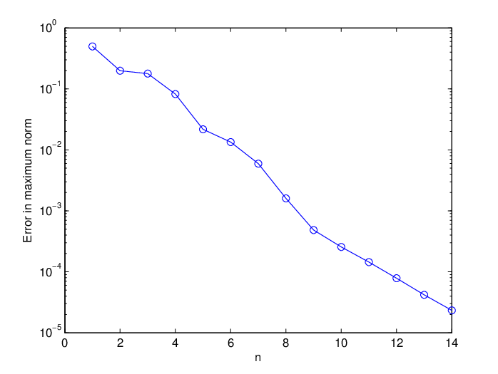
Numerical results are given in Table 2.

Table 2: Maximum errors in Galerkin solution

u_{n}

$n$	$N_{n}$	$\left\\|u-u_{n}\right\\|_{\infty}$	cond
$1$	$4$	$4.98E-1$	$1.5$
$2$	$10$	$1.99E-1$	$3.6$
$3$	$20$	$1.78E-1$	$5.7$
$4$	$35$	$8.22E-2$	$11.0$
$5$	$56$	$2.18E-2$	$17.1$
$6$	$84$	$1.34E-2$	$27.1$
$7$	$120$	$5.95E-3$	$39.4$
$8$	$165$	$1.60E-3$	$55.9$
$9$	$220$	$4.85E-4$	$75.8$
$10$	$286$	$2.56E-4$	$100.2$
$11$	$364$	$1.44E-4$	$128.9$
$12$	$455$	$7.85E-5$	$162.4$
$13$	$560$	$4.19E-5$	$200.6$
$14$	$680$	$2.33E-5$	$244.0$

The integrations in (30) were performed with (38); and the integration parameter $q$ was chosen as $q=n+2$ . Numerical experiments indicate that a larger $q$ does not change the results significantly. The condition numbers for the system (30) were again calculated with Matlab. An estimation for the error in the maximum norm was calculated on the grid given by

\left(\begin{array}[c]{r}x_{i,j,k}\\ y_{i,j,k}\\ z_{i,j,k}\end{array}\right)=\left(\begin{array}[c]{l}\frac{i}{21}\sin\left(\frac{k}{21}\pi\right)\cos\left(\frac{2j}{20}\pi\right)\\[5.69054pt] \frac{i}{21}\sin\left(\frac{k}{21}\pi\right)\sin\left(\frac{2j}{20}\pi\right)\\[5.69054pt] \frac{i}{21}\cos\left(\frac{k}{21}\pi\right)\end{array}\right),\quad i,k=1,\ldots,20,\quad j=1,\ldots,40.

The error for the Galerkin method is shown in Figure 6 and the development of the condition number is shown in Figure 7. Again the numerical experiment seems to indicate an exponential convergence of the method and a linear growth of the condition numbers with respect to the number of degrees of freedom $N_{n}$ of the linear system (30).

Additional Remarks. We present and study a spectral method for the Neumann problem

	$\displaystyle-\Delta u(\mathbf{s})+\gamma(\mathbf{s})u(\mathbf{s})$	$\displaystyle=f(\mathbf{s}),\quad\quad\mathbf{s}\in\text{$\Omega$}\subseteq\mathbb{R}^{d}\vskip 6.0pt plus 2.0pt minus 2.0pt$
	$\displaystyle\frac{\partial u(\mathbf{s})}{\partial\mathbf{n}_{\mathbf{s}}}$	$\displaystyle=g(\mathbf{s}),\quad\quad\mathbf{s}\in\partial\text{$\Omega$}$

in a forthcoming paper. We are also investigating the behaviour of the condition number for the linear system (30) associated with our spectral method, attempting to prove that it has size $\mathcal{O}(N_{n})$ , consistent with the numbers shown in Tables 1 and 2.

Our earlier numerical examples use given

\Phi:\overline{B}_{d}\underset{onto}{\overset{1-1}{\longrightarrow}}\overline{\Omega}

chosen to be nontrivial and illustrative. In general, however, when given a smooth mapping

\varphi:S\underset{onto}{\overset{1-1}{\longrightarrow}}\partial\Omega,

it may not be clear as to how to extend $\varphi$ to $\Phi$ over $B$ . In some cases there is an obvious choice, as when $\Omega$ is an ellipsoid. We are investigating schemes to produce continuously differentiable extensions $\Phi$ which satisfy

\min_{\mathbf{x}\in\overline{B}}\,\left|\det J(\mathbf{x})\right|>0

and for which $J(\mathbf{x})$ is easily computable.

References

[1] M. Abramowitz and I. Stegun, Handbook of Mathematical Functions, Dover Publications, Inc., New York, 1965.
[2] K. Atkinson, An Introduction to Numerical Analysis, 2 ${}^{\text{nd}}$ ed., John Wiley, New York, 1989.
[3] K. Atkinson and W. Han, Theoretical Numerical Analysis: A Functional Analysis Framework, 2 ${}^{\text{nd}}$ ed., Springer-Verlag, New York, 2005.
[4] K. Atkinson and O. Hanson, Solving the nonlinear Poisson equation on the unit disk, J. Integral Equations Appl., 17 (2005), 223-241.
[5] S. Brenner and L. R. Scott, The Mathematical Theory of Finite Element Methods, 2 ${}^{\text{nd}}$ ed., Springer-Verlag, New York, 2002.
[6] E. Doha and W. Abd-Elhameed, Efficient spectral-Galerkin algorithms for direct solution of second-order equations using ultraspherical polynomials, SIAM J. Sci. Comput. 24 (2002), 548-571.
[7] C. Dunkl and Y. Xu, Orthogonal Polynomials of Several Variables, Cambridge Univ. Press, Cambridge, 2001.
[8] W. Gautschi, Orthogonal Polynomials, Oxford University Press, Oxford, 2004.
[9] O. Hansen, K. Atkinson, and D. Chien, On the norm of the hyperinterpolation operator on the unit disk and its use for the solution of the nonlinear Poisson equation, IMA J. Numer. Anal., doi: 10.1093/imanum/drm052, 2008.
[10] E.W. Hobson, The Theory of Spherical and Ellipsoidal Harmonics, Chelsea Publishing Company, New York, 1965.
[11] V. Liseikin, Grid Generation Methods, Springer-Verlag, Berlin, 1999.
[12] B. Logan and L. Shepp, Optimal reconstruction of a function from its projections, Duke Math. J. 42, (1975), 645–659.
[13] T. M. MacRobert, Spherical Harmonics, Dover Publications, Inc., New York, 1948.
[14] S. Mikhlin, Mathematical Physics, An Advanced Course, North-Holland, 1970.
[15] D. Ragozin, Constructive polynomial approximation on spheres and projective spaces, Trans. Amer. Math. Soc. 162 (1971), 157-170.
[16] J. Shen, Efficient spectral-Galerkin methods IV. Spherical geometries, SIAM J. Sci. Comput. 20 (1999), 1438-1455.
[17] J. Shen and L. Wang, Analysis of a spectral-Galerkin approximation to the Helmholtz equation in exterior domains, SIAM J. Numer. Anal. 45 (2007), 1954-1978.
[18] A. Stroud, Approximate Calculation of Multiple Integrals, Prentice-Hall, Inc., Englewood Cliffs, N.J., 1971.
[19] Yuan Xu, Lecture notes on orthogonal polynomials of several variables, in Advances in the Theory of Special Functions and Orthogonal Polynomials, Nova Science Publishers, 2004, 135-188.
[20] Yuan Xu, Analysis on the unit ball and on the simplex, Electron. Trans. Numer. Anal. 25 (2006), 284-301.
[21] S. Zhang and J. Jin, Computation of Special Functions, John Wiley & Sons, Inc., New York, 1996.

A Spectral Method for Elliptic Equations: The Dirichlet Problem