Needlet Detection of Features in WMAP CMB Sky and the Impact on Anisotropies and Hemispherical Asymmetries
Abstract
We apply spherical needlets to the Wilkinson Microwave Anisotropy Probe 5-year cosmic microwave background (CMB) data_set, to search for imprints of nonisotropic features in the CMB sky. We use the needlets’ localization properties to resolve peculiar features in the CMB sky and to study how these features contribute to the anisotropy power spectrum of the CMB. In addition to the now well-known “cold spot” of the CMB map in the southern hemisphere, we also find two hot spots at greater than 99% confidence level, again in the southern hemisphere and closer to the Galactic plane. While the cold spot contributes to the anisotropy power spectrum in the multipoles between to , the hot spots are found to be dominating the anisotropy power in the range between and . Masking both the cold and the two hot spots results in a reduction by about 15% in the amplitude of the angular power spectrum of CMB around . The resulting changes to the cosmological parameters when the power spectrum is estimated masking these features (in addition to the WMAP team’s KQ85 mask) are within the 1 errors published with the WMAP mask only. We also study the asymmetry between the angular power spectra evaluated on the northern and southern hemispheres. When the features detected by needlets are masked, we find that the difference in the power, measured in terms of the anisotropy variance between and , is reduced by a factor . We make available a mask related to needlet features for more detailed studies on asymmetries in the CMB anisotropy sky.
pacs
98.80.-k, 98.80.EsI Introduction
Beyond the angular power spectrum of the cosmic microwave background (CMB) anisotropies, the high-sensitivity all-sky CMB maps produced by the Wilkinson Microwave Anisotropy Probe (WMAP)11 1 http://lambda.gsfc.nasa.gov/product/map/current/ [1] have enabled detailed statistics studies to extract higher-order information. These studies include characterizations of asymmetries in the CMB sky [2] and the search for anomalous features in the anisotropy field. Previous analyses have shown evidences for alignments [3], asymmetry in the CMB statistics between northern and southern Galactic hemispheres [4], and features such as the “cold spot,” a significant negative feature in the CMB map first identified with wavelets [5].
Wavelets can be constructed both in real space on the sphere, for instance by means of the so-called stereographic projection [6, 7, 8, 9], and in harmonic space, for instance following the prescription described in [10, 11], see also [12]. There have been already several applications of wavelets to CMB data analysis, including tests for non-Gaussianity and asymmetries [13, 14, 15, 16, 17], polarization analysis [18], foreground subtraction [19], foreground component separation [20, 21], and point source detection in CMB anisotropy maps [22]. The reason for such a wide success can be motivated as follows: the comparison between models and CMB data are primarily undertaken in the Fourier domain, where each multipole can be measured separately with all-sky experiments. However, in the presence of sky cuts data analysis must take into account the coupling among multipoles induced by the mask; statistical studies consequently become much more challenging. Wavelets address these issues by providing the possibility to combine sharp localization properties in pixel space with a peaked window function in the harmonic space.
In the latest two years, needlets have been proposed as a new wavelet system which enjoys several advantages over existing constructions. The introduction of needlets into the mathematical literature is due to [23], where their localization properties in pixel and harmonic space are established. The analysis of their statistical properties for spherical random fields is first provided by [24], where uncorrelation is discussed and it is also shown how needlets can be used to implement estimators for the angular power spectrum or tests of non-Gaussianity. The first application to WMAP data is due to [25], where needlets are used to estimate (cross-)angular power spectra in order to search for dark energy imprints on the correlation between large-scale structures and CMB. A full description of needlets and their potentiality for CMB data analysis is then provided by [26]; Ref. [27] investigates the effect of different window functions in their constructions, whereas Ref. [28] provides further mathematical results on their behavior for partially observed sky-maps. The previous results have been extended to angular power spectrum estimation in the presence of noise [29, 30], estimation of the bispectrum [31], foreground component separation [32], and analysis of directional data [33]; see also Refs. [34, 35, 36] for further developments.
Among the advantages of needlets compared to previously adopted wavelets, we recall that they are compactly supported in harmonic space, so that they allow to focus the analysis on a specific set of multipoles, which can be completely controlled [23]. Needlet coefficients can be shown to be (approximately) uncorrelated both across different frequencies and, at high multipoles, at different locations in pixel space, which makes statistical analysis much more efficient; it is possible to provide an exact analytic expression for their variance and correlation, in terms of the underlying angular power spectrum [24, 25]. Needlets do not rely on any tangent plane approximation, but they are directly embedded into the manifold structure of the sphere; they allow for direct reconstruction formulas (a consequence of the fact that they make up a tight frame system) and they are computationally very convenient [26].
In this paper, we make use of needlets to further study features in the WMAP CMB maps. We focus on the large angular scales or, equivalently, on multipoles smaller than 200. We recover the cold spot that was previously detected in WMAP data with wavelets, and we also detect other features, including two hot spots, which have so far received less attention. By masking these features, we study how the angular power spectrum of CMB anisotropies is modified. Given that these features are located in the southern hemisphere, we also discuss the extent to which these features could be responsible for the north-south asymmetry in WMAP data [37, 2, 38]. As is well known, this asymmetry has also drawn much interest in the theoretical community, since it could entail strong implications on the physical nature of primordial perturbations, including inflation [39]. By masking the low- features, we find that the difference in the CMB anisotropy variance between the two hemispheres is reduced by a factor of 2, reducing the significance of previous detections.
We also explore the evidence that statistically significant bumps and dips in the CMB anisotropy power spectrum at multipoles of 20 and 40 could be related to features in the CMB sky. We did not locate any particular feature in the sky that dominates the power spectrum at these multipoles; masking the significant features detected by needlets tuned to these multipoles did not change the power spectrum more than 5%.
The paper is organized as follows: In the following section we describe briefly the needlet formalism, then we apply it to the WMAP 5-year temperature map describing the features we observed and their significance in Sec. III. In Sec. IV we address the angular power spectrum modification induced by the specific features we measure in the temperature map, computing the effect on the cosmological parameters. We then draw our conclusion in Sec. V.
II Needlets and Search for Features
We provide here a brief summary of the needlet construction, while we refer to [26] and the references therein for a more complete discussion. We recall the spherical needlet function is defined as
| (1) |
where are the cubature points on the sphere, corresponding to the frequency and the location , and is a filter function in harmonic space. Each cubature point requires a proper weight, . Since our implementation is based on the Healpix pixelization22 2 http://healpix.jpl.nasa.gov [40], we actually compute Eq. 1 on the center of the pixels for a given resolution, following the procedure described in [25]. In this context the cubature weights can be approximated by , where is the number of pixels for the chosen Healpix resolution and k corresponds to a Healpix pixel number.
In general, needlets can be viewed as a convolution of the projection operator with suitably chosen weights provided by the function . Details on the function we used can be found in Ref. [26]. We show its profile in Fig. 1 for several values of ; in the sequel we will use the notation for . is a user-chosen parameter that characterizes the weights and then the entire set of needlets, since its value determines the width of the filter function. The choice of must be driven by the insight on the range of multipoles to be probed. Since we are interested in large angular scales, we set : this choice allows us to have eight frequencies spanning multipoles up to , while the information at smallest scales is concentrated on just three frequencies. The range of multipoles covered by each needlet is summarized in Table 1.

Since the function has a finite support in -space, by construction each needlet receives a contribution only from a specific range of multipoles, which is related to the index by a logarithmic function of . In pixel space needlets are quasiexponentially localized, due to peculiar properties of the window function , as shown by [23]. We are thus able to exploit a tight control on the localization both in terms of angular scales and directions on the sky, thus keeping a record of the signal in both domains. This makes possible the detection of specific features in the CMB map that are contributing power, for example, over a well-defined range of multipoles of the angular power spectrum.
To this aim, we first decompose the CMB temperature map onto the needlet system. As recalled before, needlets do not make up a basis, but a tight frame; however the latter enjoys all the reconstruction properties that are usually associated to bases (indeed tight frames can be simply viewed as a redundant basis). The needlet coefficients result from the projection of the temperature field on the elements of the needlet system:
| (2) | |||||
| j | -range |
|---|---|
| 1 | 2 |
| 2 | 2-5 |
| 3 | 4-10 |
| 4 | 6-18 |
| 5 | 11-33 |
| 6 | 20-60 |
| 7 | 35-108 |
| 8 | 63-196 |
| 9 | 113-352 |
| 10 | 203-635 |
| 11 | 365-1143 |
III Maps
We decomposed the Internal Linear Combination (ILC) WMAP 5-year temperature map by means of needlet functions corresponding to . As discussed in the previous section, this specific choice provides us needlets at 11 frequencies , that span properly the low multipoles we are interested in. As described above, the expression 2 can be easily represented by a map in the Healpix scheme, in which each pixel is associated with the needlet coefficient evaluated at . Figure 2 shows three clarifying examples of the WMAP 5-year ILC map decomposition on , and needlets by making use of the functions depicted in Fig. 1.
We first applied our procedure to the WMAP map with the extended mask KQ from the WMAP team. Such a large mask, however, entails a greater correlation for multipoles corresponding to large angular scales; for low values of , this could potentially impact the needlets’ coefficients as well. Any detection of significant features in the CMB anisotropy map using the large mask, however, can be reconfirmed at a higher significance level with a smaller mask. After studying the temperature map using KQ, we repeated all the analysis applying KQ, which is the mask currently favored for cosmological data analysis, including power spectrum measurements. We find that our results related to statistically significant features on the WMAP map are fully consistent in the two cases.
III.A Hot/Cold spot maps
In Fig. 2, we represent the needlet coefficients for the cases of to . These three frequencies are particularly interesting since they probe the low-multipole region, highlighting a peculiar pattern of anisotropies in the southern hemisphere. When , we recognize two spots, one hotter and one colder than the average CMB fluctuations. While the latter is a detection of the so-called cold spot, a feature studied in detail in the literature as a source of non-Gaussianity in the CMB map [41, 42, 5, 43, 44, 45, 46], the hot spot has not had the same scrutiny with only a minor description in Refs. [47, 43].


In fact, the and needlet coefficients represent a cross-validation of the existing literature, as they also highlight a second hot spot centered at (as pointed out in Ref. [47]) and a minor cold spot centered at (observed in Ref. [43]), that actually appears with an adjacent hot spot. In Fig. 3 the three spots we used in the angular power spectrum analysis are shown. We stress that our identification follows uniform criteria with the same technique, quite differently from some of the existing literature. Moreover, as explained above we are also able to identify exactly the range of multipoles where these features contribute to the angular power spectrum of CMB anisotropies, due to the specific needlet properties.


To establish the significance of the features we detected, we consider a Monte Carlo analysis by performing a large set of simulations (1000) of a Gaussian CMB sky with the same angular power spectrum as the WMAP 5-year best-fit cosmological parameters [48]; we then compute the average and the standard deviation of the distribution for each needlet coefficient. The expected distribution is Gaussian with zero mean, (see [24]), in good agreement with our simulations. We focus on the statistic
| (3) |
where is the usual standard deviation of the distribution. In Fig. 2, we show that the hot and cold spots exceed three sigma level at . The cold spot appears significantly both in the needlet coefficients for and , and thus its impact can be reckoned to span the range between and (Table 1). In Table 2 the significance values of the three anomalous spots are quoted.
| Property / Spots | Cold Spot | Hot Spot | Hot Spot |
|---|---|---|---|
| 4 | 4 | 3 | |
It may be suspected that the hot spot we located could be a spurious effect due to oscillations in the needlet function. We considered this explanation, but we concluded that the distance at which the hot and cold spot appear is greater than the needlet oscillation range. We aim at a further investigation of this issue in our ongoing work.
As a test for the joint significance of needlet coefficients, we consider the statistic
| (4) |
where is the second moment of the distribution. Of course, the statistical distribution of cannot be taken as Gaussian. Hence, to analyze its statistical significance we used again a set of Monte Carlo simulations and we followed the procedure described in Sec. III. Figure 4 shows the values of these statistics for the pair and , left panel, and for and , right panel. Results are expressed directly in terms of the statistic defined in Eq. 4 in the upper panels; in the lower panels a threshold of for is adopted to underline the fact that the hot and cold spots identified by the mask are the most significant.


III.B North-South Asymmetry
We now wish to investigate the extent in which masking the previously found features affects the asymmetry between the northern and the southern hemisphere of the CMB sky. To see this, we recall that in Refs. [24, 25, 26] it is shown that
whence is an unbiased estimator for the weighted angular power spectrum. In [24], Sec. 7, it is also shown that this statistic is approximately Gaussian (after centering and normalization) at high frequencies, see also [32, 30] for extensions and related work. Developing this idea, we computed here the total power in each hemisphere by taking the sum of squares of the needlet coefficients at and extracted from the masked ILC temperature map
| (5) |
We label the mask associated with the and features we found as “”, and we include it in addition to standard WMAP masks.
The difference is measured by computing
| (6) |
where , is the quantity in Eq. 5, where the needlet coefficients are restricted to either the northern or the southern hemisphere (in the Galactic coordinate system), normalized to the variance of the whole sky. The latter actually turn out to be the cosmic variance of the CMB power spectrum binned with . In some sense, D is measuring the difference between two local versions of the power spectrum estimator; such local estimators can indeed be rigorously justified, in view of the uncorrelation properties of needlets in pixel space (see [28]). In practice, we defined the pixels in the northern hemisphere as those outside the mask characterized by and pixels in the southern hemisphere as those outside the mask, with .
In Fig. 5 we plot as defined in Eq. 5 extracted from the whole sky as well as those measured in each hemisphere, both including the spots and masking them. The southern hemisphere shows an excess of power compared to the northern one that is reduced by a factor of 2 when the “j3j4” mask is applied. Notice that, as expected, the power measured in the north region is not affected by the masking procedure. In the lower panel of Fig. 5 we quantify this effect computing the difference , normalized to the variance of the estimator.


The results are summarized in Table 3. Our findings are sensitive to the chosen sky-cut: when the KQ mask is used, the asymmetry, measured in terms of a difference in the variance of power, decreases from without the needlet mask to with needlet mask. When the more aggressive mask KQ is applied to CMB data (together with the mask), the difference is larger and the global asymmetry is further reduced: from to . Note that the north-south power variance difference with just the WMAP team’s masks, KQ75 and KQ85, is rather small (4.26 vs 4.37); this suggests that the hemispherical asymmetry cannot be explained by simply extending the galactic plane mask. With the mask we introduced (which cuts roughly 0.5% of the sky), we find a significant reduction of a factor of 2.
Given that we mask a smaller area on the sky than the 10% difference between KQ85 and KQ75, it seems rather likely that the hemispherical asymmetry can be credited to features in the southern hemisphere. While we have localized (some of) these features, this does not establish by itself whether the asymmetry is primordial or associated with fluctuations in our local universe. There exist already several extended studies on the nature of the cold spot ([49, 50, 51, 52, 53, 45, 54]); for further statistical studies we make publicly available the mask.
| Mask | D | |||
|---|---|---|---|---|
| kq | 766 | 556 | 974 | 4.26 |
| kq+j3j4 | 673 | 544 | 802 | 1.97 |
| kq | 703 | 502 | 908 | 4.37 |
| kq+j3j4 | 655 | 492 | 728 | 2.0 |


III.C Further statistical analysis
As a further statistical cross-check, we chose randomly needlet coefficients at different locations on the map and fit their distribution to the one derived from 1000 simulations where the KQ mask was applied. The simulated results are in excellent agreement with a zero-mean Gaussian distribution, as shown in Fig. 6. This result is of course expected, as the needlet coefficients are a linear functional of the underlying temperature map. However, we report the figure as a further check to assure that the procedure we followed to compute the significance of the spots is well justified.
We followed the same procedure also to quantify the significance of . Of course, in this case simulations are indeed necessary, because is a nonlinear statistic and hence non-Gaussian. In Fig. 7 we provide some evidence on the significance of the statistics we measured in the regions where the anomalous spots are located. The curve is the fit to the distribution of needlet coefficients in simulated maps, while the vertical lines mark the value measured in the WMAP temperature needlet coefficients. The simulated distribution has rather large tails; the statistical significance of at the locations corresponding to the spots is nevertheless rather high, with an estimated p-value of for the cold spot and of for the hot spot. We can still confirm that the signal is mostly peaked in the correlation between and .


IV Impact on the CMB power spectrum
The purpose of this section is to investigate the extent in which masking the hot and cold regions we found affects the CMB power spectrum [49]. To address this issue, we first estimate the angular power spectrum from the ILC WMAP 5-year map after applying the KQ mask. We then compare this result with the angular power spectrum resulting from a wider mask: the sum of KQ plus the regions above three sigma level we discovered when performing our temperature analysis. We report in Fig. 8 the resulting mask.
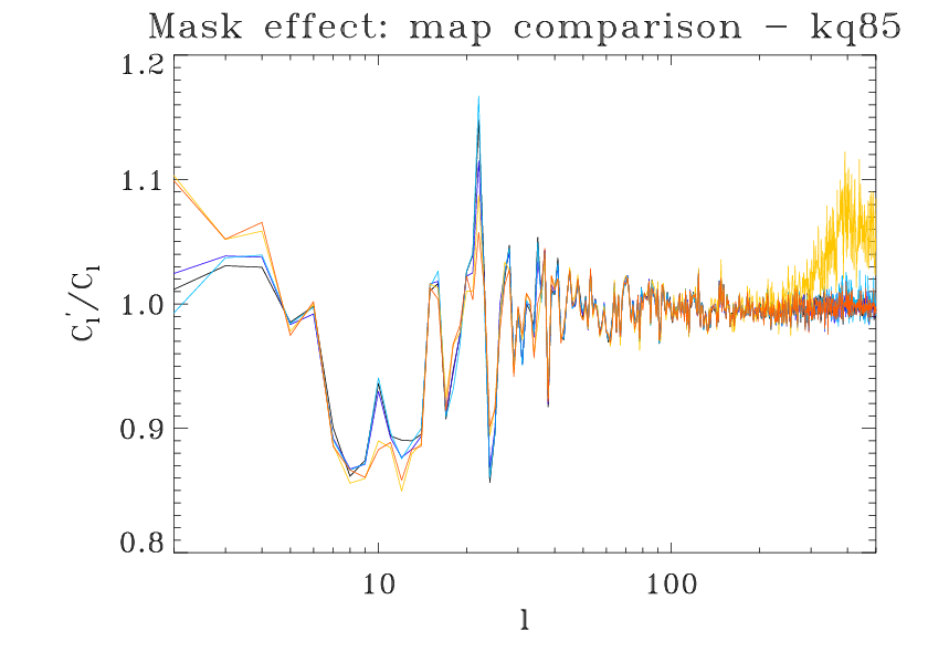
The effect of the different masking is not negligible, reaching the value of at low multipoles. To check against systematics, we performed a Monte Carlo simulation of 200 CMB maps with the underlying WMAP 5-year best-fit model [48], in order to estimate the mean effect of the joint mask. We computed the average and the standard deviation to quantify the hot/cold spots effect. The results are shown in Fig. 9.

Quite remarkably, the region where the signal is stronger is exactly the one where the cold spot is localized. This may be interpreted as a confirmation of the localization properties of needlets in pixel and harmonic spaces. We believe the use of the ILC map is justified here, because our signal peaks at low multipoles; however for completeness we computed the same quantity from both the W and V bands of WMAP 5 year, as well as using the map obtained by [55]33 3 http://space.mit.edu/home/angelica/gsm/. The result is fully consistent with what we found using ILC, thus validating the procedure we followed. The signal is shown in Fig. 10
The next step has been to evaluate the effect that the change in the angular power spectrum induces on cosmological parameter estimates. Since the low multipoles region is affected by the largest variation, we expect that changes might occur on the spectral index, , the optical depth, and possibly on the primordial fluctuation normalization amplitude . Actually, since the variation is at maximum in an handful of multipoles, we expect a global variation on the power spectrum of roughly few parts on 1000.
The WMAP team performed the temperature analysis splitting the low multipoles and the high multipoles regions. The former is probed by a Gibbs-sampling based Monte Carlo analysis [56]. The high moments are instead investigated fitting the angular power spectrum extracted from the W and V bands. To take into account the modifications due to the new masking we replaced the KQ mask used at low resolution with the joint mask KQ plus the hot and cold spots (Fig. 8), and multiplied the angular power spectrum used for the analysis by the ratio between the computed with the wider mask and obtained with the unmodified KQ mask applied to ILC, in the range of multipoles (see Fig. 10).
The results are shown in Table 4. In short, we do not observe a significant variation in any of the cosmological parameters.
| Parameter | WMAP5 | Hot/Cold spot masked () | - mask |
|---|---|---|---|
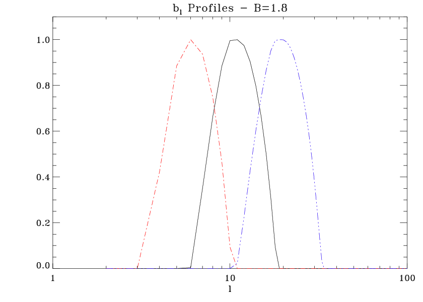
It is well known that the angular power spectrum measured by the WMAP Collaboration shows some interesting features at low multipoles; in particular the range between and has a deficit in power with respect to the prediction of the best-fit CDM theoretical model, while that between to shows excess power. To investigate these issues, we chose needlets corresponding to frequencies that match those two intervals and we looked for coefficients exceeding the threshold of three sigma. More precisely, we select and we take , to span the relevant ranges of multipoles. Figure 11 (upper panel) and Fig. 12 show (respectively) the profile employed for this purpose and the corresponding needlet coefficients.


We find that the effect on the angular power spectrum is actually rather small. However it does follow the expected sign, decreasing the deficit and the excess of power in the selected ranges. The effect is shown in the lower panel of Fig. 11.
V Conclusions
We apply spherical needlets to the Wilkinson Microwave Anisotropy Probe 5-year cosmic microwave background dataset, to search for imprints of nonisotropic features in the CMB sky.
After calibration by means of a large set of mock simulations, the analysis of needlet coefficients highlights the presence of the now well-known “cold spot” of the CMB map in the southern hemisphere, and in addition two hot spots at significance greater than 99% confidence level, again in the southern hemisphere and closer to the Galactic plane. While the cold spot primarily contributes to the anisotropy power spectrum in the multipoles between to , the hot spots are found to be dominating the anisotropy power in the range between and .
We also studied the effect the two spots have on the CMB power spectrum, by building mock CMB simulations. We conclude that, especially at low multipoles, the effect is measurable: masking both the cold and the two hot spots results in an increase in the quadrupole amplitude of 10%, while at power is reduced by 12%. To investigate the effect of this difference on the value of cosmological parameters, we modified the WMAP 5-year CMB fiducial power spectrum and the KQ mask used to perform the analysis by cutting out the contribution of the two spots, and we repeated the parameter estimation analysis. The results we obtain are slightly different, but fully consistent within the 1 errors on parameters published by the WMAP team.
Since all three spots appear in the southern hemisphere, we also studied the power spectrum asymmetry between the two hemispheres, which has been previously found to be statistically significant. When the features detected by needlets are masked, we find that the difference in the power, measured in terms of the anisotropy variance between and , is reduced by a factor of . This decreases the significance of the previously claimed north-south asymmetry. We make the mask resulting from needlet features available for future, more detailed studies on the asymmetries in the CMB anisotropy sky44 4 http://www.fisica.uniroma2.it/cosmo/masks.
Acknowledgments
DP thanks Marcella Veneziani for useful discussions and the UCI Physical Sciences Department where this work has been performed. DM is grateful to P.Baldi, G.Kerkyacharian and D.Picard for many useful discussions.
References
- [1] G. Hinshaw, J. L. Weiland, R. S. Hill, N. Odegard, D. Larson, C. L. Bennett, J. Dunkley, B. Gold, M. R. Greason, N. Jarosik, et al., ArXiv e-prints 803 (2008), eprint 0803.0732.
- [2] N. E. Groeneboom and H. K. Eriksen, ArXiv e-prints 807 (2008), eprint 0807.2242.
- [3] C. J. Copi, D. Huterer, D. J. Schwarz, and G. D. Starkman, Phys. Rev. D. 75, 023507 (2007), eprint arXiv:astro-ph/0605135.
- [4] H. K. Eriksen, A. J. Banday, K. M. Górski, F. K. Hansen, and P. B. Lilje, ApJ 660, L81 (2007), eprint arXiv:astro-ph/0701089.
- [5] M. Cruz, E. Martínez-González, P. Vielva, and L. Cayón, MNRAS 356, 29 (2005), eprint arXiv:astro-ph/0405341.
- [6] J.-P. Antoine and P. Vandergheynst, Appl. Comput. Harmon. Anal. 7, 262 (1999), ISSN 1063-5203.
- [7] Y. Wiaux, L. Jacques, and P. Vandergheynst, ApJ 632, 15 (2005), eprint arXiv:astro-ph/0502486.
- [8] J. D. McEwen, M. P. Hobson, A. N. Lasenby, and D. J. Mortlock, MNRAS 371, L50 (2006a), eprint arXiv:astro-ph/0604305.
- [9] J. D. McEwen, P. Vielva, M. P. Hobson, E. Martínez-González, and A. N. Lasenby, MNRAS 376, 1211 (2007), eprint arXiv:astro-ph/0602398.
- [10] M. Holschneider, Journal of Mathematical Physics 37, 4156 (1996).
- [11] J. D. McEwen, M. P. Hobson, and A. N. Lasenby, ArXiv Astrophysics e-prints (2006b), eprint astro-ph/0609159.
- [12] Y. Wiaux, J. D. McEwen, P. Vandergheynst, and O. Blanc, MNRAS 388, 770 (2008a), eprint 0712.3519.
- [13] P. Vielva, E. Martínez-González, R. B. Barreiro, J. L. Sanz, and L. Cayón, ApJ 609, 22 (2004a), eprint arXiv:astro-ph/0310273.
- [14] P. Cabella, F. Hansen, D. Marinucci, D. Pagano, and N. Vittorio, Phys. Rev. D 69, 063007 (2004), eprint arXiv:astro-ph/0401307.
- [15] J. D. McEwen, M. P. Hobson, A. N. Lasenby, and D. J. Mortlock, ArXiv e-prints 803 (2008), eprint 0803.2157.
- [16] Y. Wiaux, P. Vielva, R. B. Barreiro, E. Martínez-González, and P. Vandergheynst, MNRAS 385, 939 (2008b), eprint 0706.2346.
- [17] Y. Wiaux, P. Vielva, E. Martínez-González, and P. Vandergheynst, Physical Review Letters 96, 151303 (2006), eprint arXiv:astro-ph/0603367.
- [18] P. Cabella, P. Natoli, and J. Silk, Phys. Rev. D. 76, 123014 (2007), eprint arXiv:0705.0810.
- [19] F. K. Hansen, A. J. Banday, H. K. Eriksen, K. M. Górski, and P. B. Lilje, ApJ 648, 784 (2006), eprint arXiv:astro-ph/0603308.
- [20] Y. Moudden, J. . Cardoso, J. . Starck, and J. Delabrouille, EURASIP Journal of Applied Signal Processing 2005, 2437 (2005), eprint astro-ph/0407053.
- [21] J.-L. Starck, Y. Moudden, P. Abrial, and M. Nguyen, A&A 446, 1191 (2006), eprint arXiv:astro-ph/0509883.
- [22] J. L. Sanz, D. Herranz, M. Lopez-Caniego, and F. Argueso, ArXiv Astrophysics e-prints (2006), eprint astro-ph/0609351.
- [23] F. J. Narcowich, P. Petrushev, and J. D. Ward, SIAM J. Math. Anal. 38, 574 (2006), ISSN 0036-1410.
- [24] P. Baldi, G. Kerkyacharian, D. Marinucci, and D. Picard, Annals of Statistics in press (2006), eprint arXiv:math.ST/0606599.
- [25] D. Pietrobon, A. Balbi, and D. Marinucci, Phys. Rev. D 74, 043524 (2006), eprint arXiv:astro-ph/0606475.
- [26] D. Marinucci, D. Pietrobon, A. Balbi, P. Baldi, P. Cabella, G. Kerkyacharian, P. Natoli, D. Picard, and N. Vittorio, MNRAS 383, 539 (2008), eprint 0707.0844.
- [27] F. Guilloux, G. Fay, and J.-F. Cardoso, ArXiv e-prints 706 (2007), eprint 0706.2598.
- [28] P. Baldi, G. Kerkyacharian, D. Marinucci, and D. Picard, Under revision for Bernoulli ArXiv e-prints 706 (2007), eprint 0706.4169.
- [29] G. Faÿ, F. Guilloux, M. Betoule, J. . Cardoso, J. Delabrouille, and M. Le Jeune, ArXiv e-prints 807 (2008), eprint 0807.1113.
- [30] G. Fay and F. Guilloux (2008), URL http://www.citebase.org/abstract?id=oai:arXiv.org:0807.2162.
- [31] X. Lan and D. Marinucci, ArXiv e-prints 802 (2008a), eprint 0802.4020.
- [32] J. Delabrouille, J. . Cardoso, M. Le Jeune, M. Betoule, G. Fay, and F. Guilloux, ArXiv e-prints 807 (2008), eprint 0807.0773.
- [33] P. Baldi, G. Kerkyacharian, D. Marinucci, and D. Picard, ArXiv e-prints 807 (2008), eprint 0807.5059.
- [34] D. Geller and A. Mayeli (2007), URL http://www.citebase.org/abstract?id=oai:arXiv.org:0706.3642.
- [35] X. Lan and D. Marinucci, ArXiv e-prints 805 (2008b), eprint 0805.4154.
- [36] A. Mayeli (2008), URL http://www.citebase.org/abstract?id=oai:arXiv.org:0806.3009.
- [37] B. Lew, ArXiv e-prints 808 (2008), eprint 0808.2867.
- [38] F. K. Hansen, P. Cabella, D. Marinucci, and N. Vittorio, ApJ 607, L67 (2004), eprint arXiv:astro-ph/0402396.
- [39] A. L. Erickcek, M. Kamionkowski, and S. M. Carroll, ArXiv e-prints 806 (2008), eprint 0806.0377.
- [40] K. M. Górski, E. Hivon, A. J. Banday, B. D. Wandelt, F. K. Hansen, M. Reinecke, and M. Bartelmann, ApJ 622, 759 (2005), eprint arXiv:astro-ph/0409513.
- [41] P. Vielva, E. Martínez-González, R. B. Barreiro, J. L. Sanz, and L. Cayón, ApJ 609, 22 (2004b), eprint arXiv:astro-ph/0310273.
- [42] D. L. Larson and B. D. Wandelt, ApJ 613, L85 (2004), eprint arXiv:astro-ph/0404037.
- [43] P. Vielva, Y. Wiaux, E. Martínez-González, and P. Vandergheynst, MNRAS 381, 932 (2007), eprint arXiv:0704.3736.
- [44] M. Cruz, L. Cayón, E. Martínez-González, P. Vielva, and J. Jin, ApJ 655, 11 (2007), eprint arXiv:astro-ph/0603859.
- [45] M. Cruz, E. Martinez-Gonzalez, P. Vielva, J. M. Diego, M. Hobson, and N. Turok, ArXiv e-prints 804 (2008), eprint 0804.2904.
- [46] K. M. Smith and D. Huterer, ArXiv e-prints 805 (2008), eprint 0805.2751.
- [47] P. D. Naselsky, P. R. Christensen, P. Coles, O. Verkhodanov, D. Novikov, and J. Kim, ArXiv e-prints 712 (2007), eprint 0712.1118.
- [48] E. Komatsu, J. Dunkley, M. R. Nolta, C. L. Bennett, B. Gold, G. Hinshaw, N. Jarosik, D. Larson, M. Limon, L. Page, et al., ArXiv e-prints 803 (2008), eprint 0803.0547.
- [49] I. Masina and A. Notari, ArXiv e-prints 808 (2008), eprint 0808.1811.
- [50] N. Sakai and K. T. Inoue, Phys. Rev. D. 78, 063510 (2008), eprint 0805.3446.
- [51] B. R. Granett, M. C. Neyrinck, and I. Szapudi, ArXiv e-prints 805 (2008), eprint 0805.2974.
- [52] J. A. R. Cembranos, A. de la Cruz-Dombriz, A. Dobado, and A. L. Maroto, ArXiv e-prints 803 (2008), eprint 0803.0694.
- [53] R. Genova-Santos, J. A. Rubino-Martin, R. Rebolo, R. A. Battye, F. Blanco, R. D. Davies, R. J. Davis, T. Franzen, K. Grainge, M. P. Hobson, et al., ArXiv e-prints 804 (2008), eprint 0804.0199.
- [54] F. K. Hansen, H. K. Eriksen, A. J. Banday, K. M. Gorski, and P. B. Lilje, in Cosmic Frontiers, edited by N. Metcalfe and T. Shanks (2007), vol. 379 of Astronomical Society of the Pacific Conference Series, pp. 16–+.
- [55] A. de Oliveira-Costa, M. Tegmark, B. M. Gaensler, J. Jonas, T. L. Landecker, and P. Reich, MNRAS 388, 247 (2008), eprint arXiv:0802.1525.
- [56] H. K. Eriksen, I. J. O’Dwyer, J. B. Jewell, B. D. Wandelt, D. L. Larson, K. M. Górski, S. Levin, A. J. Banday, and P. B. Lilje, ApJ 155, 227 (2004), eprint arXiv:astro-ph/0407028.