Information Theory, Relative Entropy and Statistics
Bavaud F. (2009) Information Theory, Relative Entropy and Statistics.
In: Sommaruga G. (editor): Formal Theories of Information. Lecture Notes in Computer Science 5363, Springer, Berlin, pp. 54–78.
1 Introduction: the relative entropy as an epistemological functional
Shannon’s Information Theory (IT) (1948) definitely established the purely mathematical nature of entropy and relative entropy, in contrast to the previous identification by Boltzmann (1872) of his “-functional” as the physical entropy of earlier thermodynamicians (Carnot, Clausius, Kelvin). The following declaration is attributed to Shannon (Tribus and McIrvine 1971):
My greatest concern was what to call it. I thought of calling it “information”, but the word was overly used, so I decided to call it “uncertainty”. When I discussed it with John von Neumann, he had a better idea. Von Neumann told me, “You should call it entropy, for two reasons. In the first place your uncertainty function has been used in statistical mechanics under that name, so it already has a name. In the second place, and more important, nobody knows what entropy really is, so in a debate you will always have the advantage.”
In IT, the entropy of a message limits its minimum coding length, in the same way that, more generally, the complexity of the message determines its compressibility in the Kolmogorov-Chaitin-Solomonov algorithmic information theory (see e.g. Li and Vitanyi (1997)).
Besides coding and compressibility interpretations, the relative entropy also turns out to possess a direct probabilistic meaning, as demonstrated by the asymptotic rate formula (4). This circumstance enables a complete exposition of classical inferential statistics (hypothesis testing, maximum likelihood, maximum entropy, exponential and log-linear models, EM algorithm, etc.) under the guise of a discussion of the properties of the relative entropy.
In a nutshell, the relative entropy has two arguments and , which both are probability distributions belonging to the same simplex. Despite formally similar, the arguments are epistemologically contrasted: represents the observations, the data, what we see, while represents the expectations, the models, what we believe. is an asymmetrical measure of dissimilarity between empirical and theoretical distributions, able to capture the various aspects of the confrontation between models and data, that is the art of classical statistical inference, including Popper’s refutationism as a particulary case. Here lies the dialectic charm of , which emerges in that respect as an epistemological functional.
We have here attempted to emphasize and synthetize the conceptual significance of the theory, rather than insisting on its mathematical rigor, the latter being thoroughly developped in a broad and widely available litterature (see e.g. Cover and Thomas (1991) and references therein). Most of the illustrations bear on independent and identically distributed (i.i.d.) finitely valued observations, that is on dice models. This convenient restriction is not really limiting, and can be extended to Markov chains of finite order, as illustrated in the last part on textual data with presumably original applications, such as heating and cooling texts, or additive and multiplicative text mixtures.
2 The asymptotic rate formula
2.1 Model and empirical distributions
denotes the data, consisting of observations, and denotes a possible model for those data. The corresponding probability is , with
Assume (dice models) that each observation can take on discrete values, each observation being i.i.d. distributed as
is the model distribution. The empirical distribution, also called type (Csiszár and Körner 1980) in the IT framework, is
where counts the occurences of the -th category and is the sample size.
Both and are discrete distributions with modalities. Their collection form the simplex (figure 1)
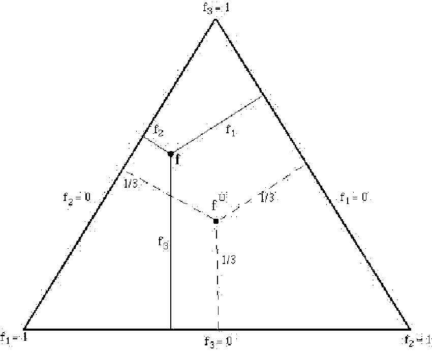
2.2 Entropy and relative entropy: definitions and properties
Let . The entropy of and the relative entropy between and are defined (in nats) as
is concave in , and constitutes a measure of the uncertainty of the outcome among possible outcomes (proofs are standard):
where
-
iff is a deterministic distribution concentrated on a single modality (minimum uncertainty)
-
iff is the uniform distribution (of the form ) (maximum uncertainty).
, also known as the Kullback-Leibler divergence, is convex in both arguments, and constitutes a non-symmetric measure of the dissimilarity between the distributions and , with
where
-
iff
-
iff is absolutely continuous with respect to , that is if implies .
Let the categories be coarse-grained, that is aggregated into groups of super-categories . Define
Then
| (1) |
2.3 Derivation of the asymptotic rate (i.i.d. models)
On one hand, straightforward algebra yields
| (2) | |||||
On the other hand, each permutation of the data yields the same . Stirling’s approximation (where means ) shows that
| (3) |
(2) and (3) imply the asymptotic rate formula:
| (4) |
Hence, is the asymptotic rate of the quantity , the probability of the empirical distribution for a given model , or equivalently the likelihood of the model for the data . Without additional constraints, the model maximizing the likelihood is simply (section 3). Also, without further information, the most probable empirical distribution is simply (section 4).
2.4 Asymmetry of the relative entropy and hard falsificationism
as a dissimilarity measure between and is proper (that is implies ) but not symmetric ( in general). Symmetrized dissimilarities such as or have often been proposed in the literature.
The conceptual significance of such functionals can indeed be questioned: from equation (4), the first argument of should be an empirical distribution, and the second argument a model distribution. Furthermore, the asymmetry of the relative entropy does not constitute a defect, but perfectly matches the asymmetry between data and models. Indeed
-
if and , then and, from (4), and, unless the veracity of the data is questioned, the model distribution should be strictly rejected
-
if on the contrary and , then and in general, and should not be rejected, at least for small samples.
Thus the theory “All crows are black” is refuted by the single observation of a white crow, while the theory “Some crows are black” is not refuted by the observation of a thousand white crows. In this spirit, Popper’s falsificationist mechanisms (Popper 1963) are captured by the properties of the relative entropy, and can be further extended to probabilistic or “soft falsificationist” situations, beyond the purely logical true/false context (see section 3.1).
2.5 The chi-square approximation
Most of the properties of the relative entropy are shared by another functional, historically anterior and well-known to statisticians, namely the chi-square . As a matter of fact, the relative entropy and the chi-square (divided by ) are identical up to the third order:
| (5) |
2.5.1 Example: coin ()
The values of the relative entropy and the chi-square read, for various and , as :
| a) | ||||
|---|---|---|---|---|
| b) | ||||
| c) | ||||
| d) | ||||
| e) | ||||
| f) |
3 Maximum likelihood and hypothesis testing
3.1 Testing a single hypothesis (Fisher)
As shown by (4), the higher , the lower the likelihood . This circumstance permits to test the single hypothesis : “the model distribution is ”. If were true, should fluctuate around its expected value , and fluctuations of too large amplitude, with occurrence probability less than (the significance level), should lead to the rejection of . Well-known results on the chi-square distribution (see e.g. Cramer (1946) or Saporta (1990)) together with approximation (5) shows to be distributed, under and for large, as with degrees of freedom.
Therefore, the test consists in rejecting at level if
| (6) |
In that respect, Fisher’s classical hypothesis testing appears as a soft falsificationist strategy, yielding the rejection of a theory for large values of . It generalizes Popper’s (hard) falsificationism which is limited to situations of strict refutation as expressed by .
3.2 Testing a family of models
Very often, the hypothesis to be tested is composite, that is of the form : “”, where constitutes a family of models containing a number of free, non-redundant parameters.
If the observed distribution itself satisfies , then there is obviously no reason to reject . But in general, and hence
| is strictly positive, with |
is known as the maximum likelihood estimate of the model, and depends on both and . We assume to be unique, which is e.g. the case if is convex.
If , follows a chi-square distribution with degrees of freedom. Hence, one rejects at level if
| (7) |
If reduces to a unique distribution , then and (7) reduces to (6). In the opposite direction, defines the saturated model, in which case (7) yields the undefined inequality .
3.2.1 Example: coarse grained model specifications
Let be a dice model, with categories . Let denote groups of categories, and suppose that the model specifications are coarse-grained (see (1)), that is
Let denote the group to which belongs. Then the maximum likelihood (ML) estimate is simply
| (8) |
3.2.2 Example: independence
Let and two categorical variables with modalities and . Let denote the joint distribution of . The distribution of alone (respectively alone) obtains as the marginal (respectively ). Let denote the set of independent distributions, i.e.
The corresponding ML estimate is
with the well-known property (where denotes the entropy associated to the empirical distribution)
| (9) |
The mutual information is the information-theoretical measure of dependence between and . Inequality insures its non-negativity. By (9), the corresponding test reduces to the usual chi-square test of independence, with degrees of freedom.
3.3 Testing between two hypotheses (Neyman-Pearson)
Consider the two hypotheses : “ ” and : “ ”, where and constitute two distinct distributions in . Let denote the rejection region for , that is such that is accepted if , and is accepted if . The errors of first, respectively second kind are
For large, Sanov’s theorem (18) below shows that
| (10) | |||
The rejection region is said to be optimal if there is no other region with and . The celebrated Neyman-Pearson lemma, together with the asymptotic rate formula (4), states that is optimal iff it is of the form
| (11) |
One can demonstrate (see e.g. Cover and Thomas (1991) p.309) that the distributions (10) governing the asymptotic error rates coincide when is optimal, and are given by the multiplicative mixture
| (12) |
where is the value insuring . Finally, the overall probability of error, that is the probability of occurrence of an error of first or second kind, is minimum for , with rate equal to
where is the value minimising the third term. The quantity , known as Chernoff information, constitutes a symmetric dissimilarity between the distributions and , and measures how easily and can be discriminated from each other. In particular, iff .
Example 2.5.1, continued: coins
Let , , and . Numerical estimates yield (in nats) , , and .
3.4 Testing a family within another
Let and be two families of models, with and . Consider the test of within , opposing : “” against : “”.
By construction, since is a more general model than . Under , their difference can be shown to follow asymptotically a chi-square distribution. Precisely, the nested test of within reads: “under the assumption that holds, rejects if
| (13) |
3.4.1 Example: quasi-symmetry, symmetry and marginal homogeneity
Flows can be represented by a square matrix such that , with the representation “ = proportion of units located at place at some time and at place some fixed time later”.
A popular model for flows is the quasi-symmetric class QS (Caussinus 1966), known as the Gravity model in Geography (Bavaud 2002a)
where quantifies the “push effect”, the “pull effect” and the “distance deterrence function”.
Symmetric and marginally homogeneous models constitute two popular alternative families, defined as
Symmetric and quasi-symmetric ML estimates satisfy (see e.g. Bishop and al. (1975) or Bavaud (2002a))
from which the values of can be obtained iteratively. A similar yet more involved procedure permits to obtain the marginal homogeneous estimates .
Example 3.4.1 continued: inter-regional migrations
Relative entropies associated to Swiss inter-regional migrations flows 1985-1990 ( cantons; see Bavaud (2002a)) are (with ) and (with ). The difference is (with only) and indicates that flows asymmetry is mainly produced by the violation of marginal homogeneity (unbalanced flows) rather than the violation of quasi-symmetry. However, the sheer size of the sample leads, at conventional significance levels, to reject all three models S , MH and QS.
3.5 Competition between simple hypotheses: Bayesian selection
Consider the set of simple hypotheses “ : ”, where for . In a Bayesian setting, denote by the prior probability of hypothesis , with . The posterior probability obtains from Bayes rule as
Direct application of the asymptotic rate formula (4) then yields
| (Bayesian hypothesis selection formula) | (15) |
which shows, for , the posterior probability to be concentrated on the (supposedly unique) solution of
In other words, the asymptotically surviving model minimises the relative entropy with respect to the long-run empirical distribution , in accordance with the ML principle.
For finite , the relevant functional is , where the second term represents a prior penalty attached to hypothesis . Attempts to generalize this framework to families of models () lie at the heart of the so-called model selection procedures, with the introduction of penalties (as in the AIC, BIC, DIC, ICOMP, etc. approaches) increasing with the number of free parameters (see e.g. Robert (2001)). In the alternative minimum description length (MDL) and algorithmic complexity theory approaches (see e.g. MacKay (2003) or Li and Vitanyi (1997)), richer models necessitate a longer description and should be penalised accordingly. All those procedures, together with Vapnik’s Structural Risk Minimization (SRM) principle (1995), aim at controlling the problem of over-parametrization in statistical modelling. We shall not pursue any further those matters, whose conceptual and methodological unification remains yet to accomplish.
3.5.1 Example: Dirichlet priors
Consider the continuous Dirichlet prior , with density , normalised to unity in , where is a vector of parameters with and . Setting , Stirling approximation yields for large.
4 Maximum entropy
4.1 Large deviations: Sanov’s theorem
Suppose data to be incompletely observed, i.e. one only knows that , where is a subset of the simplex , the set of all possible distributions with modalites. Then, for an i.i.d. process, a theorem due to Sanov (1957) says that, for sufficiently regular , the asymptotic rate of the probability that under model decreases exponentially as
| (18) |
is the so-called maximum entropy (ME) solution, that is the most probable empirical distribution under the prior model and the knowledge that . Of course, if .
4.2 On the nature of the maximum entropy solution
When the prior is uniform (), then
and minimising (over ) the relative entropy amounts in maximising the entropy (over ).
For decades (ca. 1950-1990), the “maximum entropy” principle, also called “minimum discrimination information (MDI) principle” by Kullback (1959), has largely been used in science and engineering as a first-principle, “maximally non-informative” method of generating models, maximising our ignorance (as represented by the entropy) under our available knowledge () (see in particular Jaynes (1957), (1978)).
However, (18) shows the maximum entropy construction to be justified from Sanov’s theorem, and to result form the minimisation of the first argument of the relative entropy, which points towards the empirical (rather than theoretical) nature of the latter. In the present setting, appears as the most likely data reconstruction under the prior model and the incomplete observations (see also section 5.3).
4.2.1 Example: unobserved category
Let be given and suppose one knows that a category, say , has not occured. Then
whose finiteness (for ) contrasts the behavior (for ). See example 2.5.1 f).
4.2.2 Example: coarse grained observations
4.2.3 Example: symmetrical observations
Let be a given joint model for square distributions (). Suppose one knows the data distribution to be symmetrical, i.e.
4.3 “Standard” maximum entropy: linear constraint
Let be determined by a linear constraint of the form
that is, one knows the empirical average of some quantity to be fixed to . Minimizing over the functional
| (21) |
| (22) |
where the Lagrange multiplier is determined by the constraint (see figure 2).
4.3.1 Example: average value of a dice
Suppose one believes a dice to be fair (), and one is told that the empirical average of its face values is say , instead of as expected. The value of in (22) insuring turns out to be , insuring , as well as , , , , , (Cover and Thomas (1991) p. 295).

4.3.2 Example: Statistical Mechanics
An interacting particle system can occupy configurations , a priori equiprobable (), with corresponding energy . Knowing the average energy to be , the resulting ME solution (with ) is the Boltzmann-Gibbs distribution
| (23) |
minimising the free energy , obtained (up to a constant term) by multiplying the functional (21) by the temperature . Temperature plays the role of an arbiter determining the trade-off between the contradictory objectives of energy minimisation and entropy maximisation:
-
at high temperatures (i.e. ), the Boltzmann-Gibbs distribution becomes uniform and the entropy maximum (fluid-like organisation of the matter).
-
at low temperatures (i.e. ), the Boltzmann-Gibbs distribution becomes concentrated on the ground states , making the average energy minimum (crystal-like organisation of the matter).
Example 3.4.1, continued: quasi-symmetry
ME approach to gravity modelling consists in considering flows constrained by linear constraints of the form
such that, typically
- 1)
(fixed average trip distance, cost or time )
- 2)
(fixed origin profiles, )
- 3)
(fixed destination profiles, )
- 4)
(fixed proportion of stayers)
- 5)
(balanced flows, )
Constraints 1) to 5) (and linear combinations of them) yield all the “classical Gravity models” proposed in Geography, such as the exponential decay model (with ):
Moreover, if the prior is quasi-symmetric, so is under the above constraints (Bavaud 2002a).
5 Additive decompositions
5.1 Convex and exponential families of distributions
Definition: a family of distributions is a convex family iff
Observations typically involve the identification of merged categories, and the corresponding empirical distributions are coarse grained, that is determined through aggregated values only. Such coarse grained distributions form a convex family (see table 1). More generally, linearly constrained distributions (section 4.3) are convex. Distributions (11) belonging to the optimal Neyman-Pearson regions (or ), posterior distributions (17) as well as marginally homogeneous distributions (example 3.4.1) provide other examples of convex families.
| Family | characterization | remark | convex | expon. |
|---|---|---|---|---|
| deficient | yes | yes | ||
| deterministic | yes | yes | ||
| coarse grained | yes | no | ||
| mixture | fixed | yes | yes | |
| mixture | adjustable | no | yes | |
| independent | no | yes | ||
| marginally homog. | square tables | yes | no | |
| symmetric | square tables | yes | yes | |
| quasi-symmetric | , | square tables | no | yes |
Definition: a family of distributions is an exponential family iff
Exponential families are a favorite object of classical statistics. Most classical discrete or continuous probabilistic models (log-linear, multinomial, Poisson, Dirichlet, Normal, Gamma, etc.) constitute exponential families. Amari (1985) has developed a local parametric characterisation of exponential and convex families in a differential geometric framework.
5.2 Factor analyses
Independence models are exponential but not convex (see table 1): the weighted sum of independent distributions is not independent in general. Conversely, non-independent distributions can be decomposed as a sum of (latent) independent terms through factor analysis. The spectral decomposition of the chi-square producing the factorial correspondence analysis of contingency tables turns out to be exactly applicable on mutual information (9) as well, yielding an “entropic” alternative to (categorical) factor analysis (Bavaud 2002b).
Independent component analysis (ICA) aims at determining the linear transformation of multivariate (continuous) data making them as independent as possible. In contrast to principal component analysis, limited to the second-order statistics associated to gaussian models, ICA attempts to take into account higher-order dependencies occurring in the mutual information between variables, and extensively relies on information-theoretic principles, as developed in Lee et al. (2000) or Cardoso (2003) and references therein.
5.3 Pythagorean theorems
The following results, sometimes referred to as the Pythagorean theorems of IT, provide an exact additive decomposition of the relative entropy:
Decomposition theorem for convex families: if is a convex family, then
| (24) |
where is the ME distribution for with prior .
Decomposition theorem for exponential families: if is an exponential family, then
| (25) |
where is the ML distribution for with data .
Sketch of the proof of (24) (see e.g. Simon 1973): if is convex with , its elements are of the form , which implies the maximum entropy solution to be of the form . Substituting this expression and using proves (24).
Sketch of the proof of (25) (see e.g. Simon 1973): if is exponential with , its elements are of the form (where the partition function insures the normalisation), containing free non-redundant parameters . Substituting this expression and using the optimality condition for all proves (25).
Equations (24) and (25) show that and can both occur as left and right arguments of the relative entropy, underlining their somehow hybrid nature, intermediate between data and models (see section 4.2).
5.3.1 Example: nested tests
5.3.2 Example: conditional independence in three-dimensional tables
Let with be the empirical distribution associated to the = “number of individuals in the category of , of and of ”. Consider the families of models
Model expresses that is independent from and (denoted ). Model expresses that and are independent (). Model expresses that, conditionally to , and are independent (). Models and are exponential (in ), and is exponential in the space of joint distributions on . They constitute well-known examples of log-linear models (see e.g. Christensen (1990)).
Maximum likelihood estimates and associated relative entropies obtain as (see example 3.2.2)
and permit to test the corresponding models as in (7). As a matter of fact, the present example illustrates another aspect of exact decomposition, namely
where df denotes the appropriate degrees of freedom for the chi-square test (7).
5.4 Alternating minimisation and the EM algorithm
5.4.1 Alternating minimisation
Maximum likelihood and maximum entropy are particular cases of the general problem
| (26) |
Alternating minimisation consists in defining recursively
| (27) | |||||
| (28) |
Starting with some (or some ), and for and convex, converges towards (26) (Csiszár (1975); Csiszár and Tusnády, 1984).
5.4.2 The EM algorithm
Problem (27) is easy to solve when is the coarse grained family , with solution (20) and the result (see example 4.2.2).
The present situation describes incompletely observed data, in which only (and not ) is known, with corresponding model in . Also
which shows to be the solution of . This particular version of the alternating minimisation procedure is known as the EM algorithm in the literature (Dempster et al. 1977), where (27) is referred to as the “expectation step” and (28) as the “maximisation step”.
Of course, the above procedure is fully operational provided (28) can also be easily solved. This occurs for instance for finite-mixture models determined by fixed distributions (with for ), such that the categories read as product categories of the form with
where the “mixing proportions” are freely adjustable. Solving (28) yields
which converges towards the optimal mixing proportions , unique since is convex. Continuous versions of the algorithm (in which represents a position in an Euclidean space) generate the so-called soft clustering algorithms, which can be further restricted to the hard clustering and -means algorithms. However, the distributions used in the latter cases generally contain additional adjustable parameters (typically the mean and the covariance matrix of normal distributions), which break down the convexity of and cause the algorithm to converge towards local minima.
6 Beyond independence: Markov chain models and texts
As already proposed by Shannon (1948), the independence formalism can be extended to stationary dependent sequences, that is on categorical time series or “textual” data , such as
=bbaabbaabbbaabbbaabbbaabbaabaabbaabbaabbaabbaabbaabbaabb
aabaabbaabbbaabaabaabbbaabbbaabbaabbaabbaabaabbbaabbbaabbaa
baabaabbaabaabbaabbaabbbaabbaabaabaabbaabbbbaabbaabaabaabaa
baabaabaabbaabbaabbaabbbbaab
In this context, each occurence constitutes a letter taking values in a state space , the alphabet, of cardinality . A sequence of letters is an -gram. In our example, , , , , etc.
6.1 Markov chain models
A Markov chain model of order is specified by the conditional probabilities
is the probability that the symbol following the -gram is . It obtains from the stationary distributions and as
The set of models of order constitutes an exponential family, nested as for all . In particular, denotes the independence models, and the ordinary (first-order) Markov chains.
The corresponding empirical distributions give the relative proportion of -grams in the text . They obtain as
where counts the number of occurrences of in . In the above example, the tetragrams counts are for instance:
| aaaa | 0 | aaab | 0 | aaba | 16 |
|---|---|---|---|---|---|
| aabb | 35 | abaa | 16 | abab | 0 |
| abba | 22 | abbb | 11 | baaa | 0 |
| baab | 51 | baba | 0 | babb | 0 |
| bbaa | 35 | bbab | 0 | bbba | 11 |
| bbbb | 2 | total | 199 |
6.2 Simulating a sequence
Under the assumption that a text follows a -order model , empirical distributions (with ) converge for large to . The latter define in turn -order transition probabilities, allowing the generation of new texts, started from the stationary distribution.
6.2.1 Example
The following sequences are generated form the empirical probability transitions of the Universal declaration of Human Rights, of length with states (the alphabet + the blank, without punctuation):
(independent process)
iahthire edr pynuecu d lae mrfa ssooueoilhnid nritshfssmo
nise yye noa it eosc e lrc jdnca tyopaooieoegasrors c hel
niooaahettnoos rnei s sosgnolaotd t atiet
(first-order Markov chain)
erionjuminek in l ar hat arequbjus st d ase scin ero tubied
pmed beetl equly shitoomandorio tathic wimof tal ats evash
indimspre tel sone aw onere pene e ed uaconcol mo atimered
(second-order Markov chain)
mingthe rint son of the frentery and com andepent the halons
hal to coupon efornitity the rit noratinsubject will the the
in priente hareeducaresull ch infor aself and evell
(third-order Markov chain)
law socience of social as the right or everyone held
genuinely available sament of his no one may be enties the
right in the cons as the right to equal co one soveryone
(fourth-order Markov chain)
are endowed with other means of full equality and to law no one
is the right to choose of the detent to arbitrarily in science
with pay for through freely choice work
(ninth-order Markov chain)
democratic society and is entitled without interference
and to seek receive and impartial tribunals for acts violating
the fundamental rights indispensable for his
Of course, empirical distributions are expected to accurately estimate model distributions for large enough, or equivalently for small enough, typically for
Simulations with above about (here roughly equal to 2) are over-parameterized: the number of parameters to be estimated exceeds the sample abilities to do so, and simulations replicate fragments of the initial text rather than typical -grams occurences of written English in general, providing a vivid illustration of the curse of dimensionality phenomenon.
6.3 Entropies and entropy rate
The -gram entropy and the conditional entropy of order associated to a (model or empirical) distribution are defined by
The quantity is non-increasing in . Its limit defines the entropy rate, measuring the conditional uncertainty on the next symbol knowing the totality of past occurrences:
By construction, , and the so-called redundancy satisfies .
The entropy rate measures the randomness of the stationary process: (i.e. ) characterizes a maximally random process is, that is a dice model with uniform distribution. The process is ultimately deterministic iff (i.e. ).
Shannon’s estimate of the entropy rate of the written English on symbols is about bits per letter, that is nat, corresponding to : hundred pages of written English are in theory compressible without loss to pages. Equivalently, using an alphabet containing symbols only (and the same number of pages) is in principle sufficient to code the text without loss.
6.3.1 Example: entropy rates for ordinary Markov chains
For a regular Markov chain of order 1 with transition matrix and stationary distribution , one gets
Identity holds iff , that is if the process is of order . Also, iff tends to a permutation, that is iff the process becomes deterministic.
6.4 The asymptotic rate for Markov chains
Under the assumption of a model of order , the probability to observe is
where finite “boundary effects”, possibly involving the first or last symbols of the sequence, are here neglected. Also, noting that a total of permutations of the sequence generate the same , taking the logarithm and using Stirling approximation yields the asymptotic rate formula for Markov chains
| (29) |
| where | ||
Setting returns the asymptotic formula (4) for independence models.
6.5 Testing the order of an empirical sequence
For , write as where and . Consider -order models of the form . It is not difficult to prove the identity
| (30) |
As an application, consider, as in section 3.4 , the log-likelihood nested test of within , opposing : “” against : “”. Identities (29) and (30) lead to the rejection of if
| (31) |
6.5.1 Example: test of independence
6.5.2 Example: sequential tests
For and , inequality (31) implies that the model at least of order . Setting (with ) constitutes a sequential procedure permitting to detect the order of the model, if existing.
For instance, a binary Markov chain of order and length in can be simulated as , where are i.i.d. variables uniformly distributed as , and if and if . Application of the procedure at significance level for is summarised in the following table, and shows to correctly detect the order of the model:
| df | ||||
|---|---|---|---|---|
| 0.692 | 0.00 | 1 | 3.84 | |
| 0.692 | 2.05 | 2 | 5.99 | |
| 0.691 | 110.59 | 4 | 9.49 | |
| 0.637 | 12.29 | 8 | 15.5 | |
| 0.631 | 18.02 | 16 | 26.3 |
6.6 Heating and cooling texts
Let (with and ) denote a conditional distribution of order . In analogy to formula (23) of Statistical Mechanics, the distribution can be “heated” or “cooled” at relative temperature to produce the so-called annealed distribution
Sequences generated with the annealed transitions hence simulate texts possessing a temperature relatively to the original text.
6.6.1 Example: simulating hot and cold English texts
Conditional distributions of order 3, retaining tetragram structure, have been calibrated from Jane Austen’s novel Emma (1816), containing tokens belonging to types (the alphabet, the blank, the hyphen and the apostrophe). A few annealed simulations are shown below, where the first trigram was sampled from the stationary distribution (Bavaud and Xanthos, 2002).
(original process)
feeliciousnest miss abbon hear jane is arer that isapple did
ther by the withour our the subject relevery that amile
sament is laugh in ’ emma rement on the come februptings he
(10 times hotter)
torables - hantly elterdays doin said just don’t check comedina
inglas ratefusandinite his happerall bet had had habiticents’
oh young most brothey lostled wife favoicel let you cology
(100 times hotter): any transition having occurred in the original text tends to occur again with uniform probability, making the heated text maximally unpredictable. However, most of the possible transitions did not occur initially, which explains the persistence of the English-like aspect.
et-chaist-temseliving dwelf-ash eignansgranquick-gatefullied
georgo namissedeed fessnee th thusestnessful-timencurves -
him duraguesdaird vulgentroneousedatied yelaps isagacity in
(2 times cooler) : conversely, frequent (rare) transitions become even more frequent (rare), making the text fairly predictable.
’s good of his compassure is a miss she was she come to the
of his and as it it was so look of it i do not you with her
that i am superior the in ther which of that the half - and
(4 times cooler): in the low temperature limit, dynamics is trapped in the most probable initial transitions and texts properly become crystal-like, as expected from Physics (see example 4.3.2):
ll the was the was the was the was the was the was the was
the was the was the was the was the was the was the was the
was the was the was the was the was the was the was the was
6.7 Additive and multiplicative text mixtures
In the spirit of section 5.1, additive and multiplicative mixtures of two conditional distributions and of order can be constructed as
where and . The resulting transition exists if it exists in at least one of the initial distributions (additive mixtures) or in both distributions (multiplicative mixtures).
6.7.1 Example: additive mixture of English and French
Let denote the empirical distribution of order 3 of example (6.6.1), and define as the corresponding distribution estimated on the first symbols of the French novel La bête humaine from Emile Zola. Additive simulations with various values of read (Bavaud and Xanthos, 2002):
ll thin not alarly but alabouthould only to comethey had be
the sepant a was que lify you i bed at it see othe to had
state cetter but of i she done a la veil la preckone forma feel
daband shous ne findissouservait de sais comment do be certant
she cette l’ideed se point le fair somethen l’autres jeune suit
onze muchait satite a ponded was si je lui love toura
les appelleur voice the toodhould son as or que aprennel un
revincontait en at on du semblait juge yeux plait etait
resoinsittairl on in and my she comme elle ecreta-t-il avait
autes foiser
showing, as expected, a gradual transformation from English- to French-likeness with increasing .
6.7.2 Example: multiplicative mixture of English and French
Applied now on multiplicative mixtures, the procedure described in example 6.7.1 yields (Bavaud and Xanthos, 2002)
licatellence a promine agement ano ton becol car emm*** ever
ans touche-***i harriager gonistain ans tole elegards intellan
enour bellion genea***he succept wa***n instand instilliaristinutes
n neignit innerable quit tole ballassure cause on an une grite
chambe ner martient infine disable prisages creat mellesselles
dut***grange accour les norance trop mise une les emm***
es terine fille son mainternistonsidenter ing sile celles
tout a pard elevant poingerent une graver dant lesses
jam***core son luxu***que eles visagemensation lame cendance
where the symbol *** indicates that the process is trapped in a trigram occuring in the English, but not in the French sample (or vice versa). Again, the French-likeness of the texts increases with . Interestingly enough, some simulated subsequences are arguably evocative of Latin, whose lexicon contains an important part of the forms common to English and French.
From an inferential point of view, the multiplicative mixture is of the form (12), and hence lies at the boundary of the optimal Neyman-Pearson decision region, governing the asymptotic rate of errors of both kinds, namely confounding French with English or English with French.
7 Bibliography
-
Amari, S.-I. Differential-Geometrical Methods in Statistics, Lecture Notes in Statistics 28, Springer (1985)
-
Bavaud, F. The Quasisymmetric Side of Gravity Modelling, Environment and Planning A, 34, pp.61-79 (2002a)
-
Bavaud, F. Quotient Dissimilarities, Euclidean Embeddability, and Huygens’s Weak Principle, in Classification, Clustering and Data Analysis Jajuga, K., Solkolowski, A. and Bock, H.-H. (Eds.), pp.195-202, Springer (2002b)
-
Bavaud, F. and Xanthos, A. Thermodynamique et Statistique Textuelle: concepts et illustrations, in Proceedings of JADT 2002 (6èmes Journées internationales d’Analyse statistique des Données Textuelles), St-Malo, (2002)
-
Billingsley, P. Statistical Inference for Markov Processes, University of Chicago Press, Chicago (1961)
-
Bishop, Y.M.M., Fienberg, S.E. and Holland, P.W. Discrete multivariate Analysis, The MIT Press, Cambridge, (1975)
-
Boltzmann, L. Weitere Studien über das Wärmegleichgewicht unter Gasmolekülen, Sitzungsberichte der Akademie der Wissenschaften 66 pp.275-370 (1872)
-
Cardoso, J.-F. Dependence, Correlation and Gaussianity in Independent Component Analysis, Journal of Machine Learning Research 4 pp.1177-1203 (2003)
-
Caussinus, H. Contribution à l’analyse statistique des tableaux de corré-lation, Annales de la Faculté des Sciences de Toulouse 29 pp.77-183 (1966)
-
Christensen, R. Log-Linear Models, Springer (1990)
-
Cover, T.M. and Thomas, J.A. Elements of Information Theory, Wiley (1991)
-
Cramer, H. Mathematical Methods of Statistics, Princeton University Press (1946)
-
Csiszár, I. -Divergence Geometry of Probability Distribution and Minimization Problems, The Annals of Probability 3, pp.146-158 (1975)
-
Csiszár, I. and Körner, J. Towards a general theory of source networks, IEEE Trans. Inform. Theory 26, pp.155-165 (1980)
-
Csiszár, I. and Tusnády, G. Information Geometry and Aternating Minimization Procedures, Statistics and Decisions, Supplement Issue 1 pp.205-237 (1984)
-
Dempster, A.P., Laird, N.M and Rubin, D.B. Maximum Likelihood from Incomplete Data via the EM Algorithm, J. Roy. Stat. Soc. B 39 pp.1-22 (1977)
-
Ferguson, T.S. Prior Distributions on Spaces of Probability Measures, The Annals of Statistics 2 pp.615-629 (1974)
-
Jaynes, E.T. Information theory and statistical mechanics, Physical Review 106 pp.620-630 and 108 pp.171-190 (1957)
-
Jaynes, E.T. Where do we stand on maximum entropy?, presented at the Maximum Entropy Formalism Conference, MIT, May 2-4 (1978)
-
Kullback, S. Information Theory and Statistics, Wiley (1959)
-
Lee, T.-W., Girolami, M., Bell, A.J. and Sejnowski, T.J. A unifying Information-Theoretic Framework for Independent Component Analysis, Computers and Mathematics with Applications 39 pp.1-21 (2000)
-
Li, M. and Vitanyi, P. An Introduction to Kolmogorov complexity and its applications, Springer (1997)
-
MacKay, D.J.C. Information Theory, Inference and Learning Algorithms, Cambridge University Press (2003)
-
Popper, K. Conjectures and Refutations, Routledge (1963)
-
Robert, C.P. The Bayesian Choice, second edition, Springer (2001)
-
Sanov, I.N. On the probability of large deviations of random variables, Mat. Sbornik 42 pp.11-44 (1957) (in Russian. English translation in Sel. Trans. Math. Statist. Probab. 1 pp.213-244 (1961))
-
Saporta, G. Probabilités, Analyse de Données et Statistique, Editions Technip, Paris, (1990)
-
Simon, G. Additivity of Information in Exponential Family Power Laws, Journal of the American Statistical Association, 68, pp.478-482 (1973)
-
Shannon, C.E. A mathematical theory of communication, Bell System Tech. J. 27, pp.379-423; 623-656 (1948)
-
Tribus, M. and McIrvine, E.C. Energy and Information, Scientific American 224 pp 178-184 (1971)
-
Vapnik, V.N. The Nature of Statistical Learning Theory, Springer, (1995)