State reduction dynamics in a simplified QED model
Abstract
A simplified model of quantum electrodynamics involving a charged two-state system interacting with an electromagnetic field mode is examined. By extending the Schrödinger equation to include stochastic and nonlinear terms the dynamical process of quantum state reduction can be represented. A specific choice of modified Schrödinger dynamics is shown to result in stable coherent field states. The two-state system undergoes an induced state reduction to a generalised current state due to its interaction with the field mode. Numerical results are presented demonstrating state reduction dynamics for an initial superposition of two current states. An induced reduction time-scale for the two-state system is derived and confirmed by the numerics.
pacs
03.65.Ta, 12.20.-mI Introduction
Standard quantum dynamics cannot describe how a particular measured outcome is realised in an experiment—this feature underlies our failure to unify classical physics with its quantum roots. A direct response to this problem is to take the view that standard quantum theory is incomplete and that a complete quantum theory should provide a dynamical description of quantum state reduction. In this way it is hoped to provide an objective description of quantum measurement without recourse to a classical measuring device.
The great success of quantum theory does not leave much room to manoeuvre when proposing alternatives. Any new theory must agree with the experimentally verified predictions of quantum theory. This roughly implies that the dynamics should reduce to Schrödinger dynamics for micro systems and that state reduction effects should become more important with system size. More specifically, the form of any modifications we make should involve a random factor (at some level of approximation) to reflect the random nature of state reduction, and we would expect some nonlinearity in the dynamics, reflecting a feedback from the state vector to the probability of the outcome [1].
These features can be adequately represented by a stochastic differential equation for the quantum state [2, 3] (for general reviews see [4, 5]), the most well known model of this type being the continuous spontaneous localisation (CSL) model [6]. In the CSL model, state reduction occurs onto a basis of smeared position states leading to definite localised positions for systems of macroscopic size. However, there is scope for further model building, principally because we can choose from many other preferred bases for state reduction (e.g. [8, 7, 9]). Until we have observational evidence of state reduction dynamics we are free to experiment with different proposals.
Here we investigate the state reduction process for a simplified form of quantum electrodynamics. We consider a charged two-state quantum system interacting with a quantum electromagnetic field mode. We investigate a model which describes state reduction onto a coherent field state basis. State reduction for the two-state system happens indirectly via standard interaction with the field mode. We find that the two-state system evolves towards a generalised current eigenstate.
The appealing feature of this model is that the stable eigenstates of the system are a natural description of the classical world whereby the field is represented by a coherent state and the two-state system (representative of charged matter) by a current eigenstate. Modifications to Schrödinger’s equation only involve the field mode—it is not necessary to make further modifications in order to independently describe state reduction in the two-state system. Also, it is possible to generalise the model to field theory without generating infinite particle creation [10] (this is a problem which appears, e.g., with the CSL model [11, 12]), although it should be pointed out that this results in a loss of Lorentz invariance.
The idea that dynamical state reduction might be induced from one field to another is not new. It has appeared in previous attempts to describe state reduction in fermionic field theory by invoking a scalar field with state reduction properties to which the fermion is coupled [11, 12]. To our knowledge the process has not been previously studied in numerical detail.
In the next section we outline our model, detailing the Hamiltonian for our simplified QED system and the modified stochastic dynamics of the state vector. In section III we consider the evolution of a specific initial state vector composed of a superposition of current states. We outline the state reduction process and derive a characteristic time-scale. In section IV we present some numerical results which confirm the analytic results and intuition gained in section III. We end with some conclusions.
II The model
II.1 QED Hamiltonian
Our simplified QED Hamiltonian is given by
| (1) |
The s are the standard Pauli matrices and , are the annihilation and creation operators for a standard harmonic oscillator. The parameters , , and are constants which we interpret as the field mode frequency, the two-state energy gap, and the coupling respectively.
Models of this type are commonly used in quantum optics to describe the interaction of a two-state atom with an electromagnetic field [13]. In particular, a further approximation to the interaction term to exclude processes such as those where a photon is created as the atom is exited (the rotating wave approximation), leads to the celebrated Jaynes-Cummings model. Alternatively, this model can be derived from full QED by restricting space to just two points (time remains continuous) and considering only one photon polarisation. The result is two fermion states and one field mode. This simplification is inadequate for a number of reasons. Most importantly, the model can no longer be described as a gauge theory as there is no local symmetry associated with the fermion field. We also lose the concepts of conserved 4-current and relativistic invariance.
On the other hand, our simplified Hamiltonian has the structure of the QED Hamiltonian: it is composed of free matter and field parts and an interaction between a current operator and the field. (That corresponds to the current can be seen as we restrict full QED to a space of two points.) These features suffice in order to make a tentative attempt to understand quantum state reduction in QED.
II.2 Stochastic Schrödinger equation
We shall consider a modified Schrödinger equation of the form
| (2) |
where is a constant coupling parameter with units of and
| (3) |
The complex Wiener process satisfies , and [17]. Note that the Schrödinger equation is recovered by setting and that the additional -dependent terms only involve field operators.
Equation (2) is a stochastic differential equation for the state. It can be derived by looking for a state diffusion process describing stochastic fluctuations in the quantum probability amplitudes of possible -eigenstates [4]. The probabilities for the stochastic fluctuations must be given by the quantum probabilities at each point in time. This ensures that stochastic outcomes match with the initial quantum predictions (and leads to nonlinearity). The equation has the property that general states evolve towards -eigenstates on a time-scale approximately inversely proportional to the variance in (see below).
Using the rules of Itô calculus we can show that
| (4) |
i.e. the norm of the state is preserved under the dynamics (2). This allows us to maintain the quantum interpretation of the state as a probability amplitude.
The process for the conditional expectation of is found to be
| (5) |
where and we have used the convenient notation . When the state is an -eigenstate, the process is nonstochastic. In this case, the effect of the modifications to Schrödinger’s equation is a decay in the magnitude of at a rate given by . This can be interpreted as being due to the fact that the classical stochastic process in equation (2) is only coupled to photon annihilation events. This results in a gradual loss of energy. Appropriate tuning of is required to ensure that field energy loss is negligible whilst state reduction timescales are appropriately small for strong fields [10].
In order to demonstrate the state reducing properties of equation (2) we consider the conditional variance in defined by
| (6) |
The conditional variance process is found to be
| (7) | |||||
The first line on the right side is the effect on due to the interaction between the two-state system and field. We see that increases if there is a negative conditional covariance between and . As increases, other terms on the right side of equation (7) become more important.
If we ignore the interaction with the two-state system the variance process is a super-martingale. Integrating and taking the unconditional expectation of equation (7) we then find
| (8) |
This demonstrates that the expected variance will decrease in time and therefore that the field approaches an -eigenstate.
We can estimate the time-scale for state reduction to an -eigenstate from the following:
| (9) |
By freezing the stochastic terms on the right side of equation (8) at time we find
| (10) |
Even though must be very small to prevent energy loss, the reduction time-scale can be small if the variance in is large. This demonstrates the specific way in which the effectiveness of state reduction is dependent on the size of the system. A superposition of greatly differing -eigenstates has large variance and state reduction will occur rapidly; if then state reduction takes an extremely long time due to the small value of . In principle, the dependence of the reduction time on the -variance is a testable result. An experiment designed to test this might look for diminishing quantum interference as a signature of the state reduction [18]. The technical difficulty would be to eliminate any environmental influence.
In order to see that stochastic probabilities for outcomes match with the initial quantum estimates we consider an initial superposition of coherent states
| (11) |
where it is supposed that the coherent states , where , are sufficiently separated in phase space that (this requires that for ). We assume for simplicity that since we wish to focus on the reduction dynamics.
Note that the coherent states are eigenstates of all terms in the evolution equation (2) except the term . This means that most terms in the evolution equation simply modify the coefficients , leaving the set of states intact. The term is responsible for diffusing the initial set of coherent states. In order to analyse its effects, consider a state evolution involving just this term:
| (12) |
This equation has the solution
| (13) |
This indicates that the individual coherent state contributions to the overall superposition will decay to the ground state on a timescale . For times we can ignore this effect and assume that the set of coherent states contributing to the superposition is fixed as . From equation (10) we see that for large -variance. We can therefore assume that in the region , the state has reduced to one of the coherent states .
We can define an approximate coherent state projection operator by . For the conditional expectation is approximately either 1 or 0 depending on whether the state is reduced to or not. From equation (2) we find
| (14) |
from which we conclude that
| (15) |
valid for . The left hand equality gives the initial quantum probability for the outcome ; the right hand equality gives the stochastic probability for the same outcome.
III An experiment
Consider an initial situation where the field is in a coherent state and the two-state system is in a superposition of current () eigenstates:
In order to understand the behaviour of this model without explicitly solving it we consider some possible scenarios depending on the relative sizes of the model parameters.
Since the field state is initially coherent, the variance in is initially small. As this is our measure of system size, we can assume that equation (2) initially reduces to the Schrödinger equation.
III.1 , domination
First consider the case where the coupling tends to zero. We then have
where
| (26) |
Here we find independent state-space rotations for the two-state system and the field.
III.2 domination
Next consider the case where the field frequency and the two-state energy gap tend to zero. In this limit we find the following solution to the Schrödinger equation
where are real-valued phase factors. The interaction between two-state system and field leads to a correlation between current eigenstates and field coherent states.
These two limits provide an overall picture of two competing processes. When the interaction is dominant, different current eigenstates become associated with different coherent field states. When the interaction is negligible we find that current states rotate into one another.
III.3 domination
Consider the scenario . From equation (III.2) we can estimate the growth of variance in :
| (32) |
and the conditional covariance between and :
| (33) | |||||
(the approximation results from the fact that we have assumed that different coherent states are nearly orthogonal). As the variance grows, -effects come to dominate the evolution. This can be seen from equations (32) and (33) by noting that the and terms in equation (7) will soon outgrow the term. Let us define an approximate time at which a transition from to -dominated behaviour happens. Once in the -dominated phase, the -variance will tend to zero on a time-scale given by equation (10). The stochastic evolution effectively chooses between the possible states and leading towards a definite field coherent state and a definite current state.
Using (10) and (32) we find that a total state reduction time-scale for the current state is given by
| (34) |
In order to determine we find the value which minimises . Setting
| (35) |
therefore
| (36) |
This is the characteristic time-scale for state reduction of a superposition of current eigenstates in a two-state system coupled to a field mode.
IV Numerical results


In order to test these results we have implemented a numerical simulator. Starting from an initial state of the form given in equation (III) with coefficients and with , we have evolved the state according to equation (2). Figures 1 and 2 show sample paths for and respectively. Here we have chosen , , . This choice of parameters are such that dominates the initial evolution. The parameter is chosen to be large enough to observe state reduction for the modestly sized numerical system, but small enough that energy loss is not too significant.
It is seen that the -variance initially grows smoothly, approximately proportional to (see equation (32)). After a certain time the evolution becomes dominated by stochastic movements with a notable downward drift. The -variance finally becomes stable again as its value tends to zero (at around ).
The current in figure 2 corresponds to the same sample. It is seen that the two-state system tends stochastically towards a definite current state—in this particular case . This happens at the same time as the -variance goes to zero.

We define the reduction time in our numerics as the stopping time at which , i.e.
| (37) |
Figure 3 shows numerical estimates of the expectation of this stopping time for a range of values. Other parameters are chosen to be and . Expectations are determined using 100 sample paths for each point. The estimates are seen to almost perfectly fit the curve with . This confirms the form of the characteristic state reduction time given in equation (36). The error bars indicate a range of one standard deviation for . We observe that the variance in the stopping time decreases as increases.
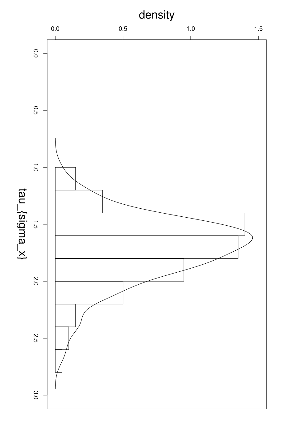
Figure 4 shows a histogram of results for 100 sample paths with . Also shown is the Gaussian kernel density estimate [19]. The distribution of stopping times is approximately normal with a slight skew. The important result is that the density of events with large deviation from the mean stopping time falls away rapidly.
We find that occurrences of and are even to within statistical error. This agrees with standard quantum predictions for a measurement of given the initial conditions.
V Conclusions
We have investigated the state reduction dynamics described by a modified Schrödinger equation for a simplified QED system. Our simplified QED system is composed of a charged two-state system interacting with an electromagnetic field mode. The modified dynamics result in state reduction to an over-complete coherent field state basis. At the same time, the electromagnetic interaction leads to the development of correlation between current states and field coherent states. This leads to an induced state reduction to a current state basis for the two-state system. We have considered evolution from a specific initial condition composed of an equal superpostion of the two possible current eigenstates with a coherent field state. We have implemented a numerical simulator to generate sample state evolutions. These have confirmed our analytic predictions for the general behaviour and the time-scales involved.
The time-scale for state reduction of the the two-state system is found to behave as . We might speculatively suggest that the reduction time-scale for more general charged matter systems might scale as for 4-current .
Acknowledgements
I would like to thank Philip Pearle and Dorje Brody for useful comments.
References
- [1] P. Pearle, Phys. Rev. D13, (1976) 857.
- [2] P. Pearle, Intl. J. Theo. Phys. 18, (1979) 489.
- [3] N. Gisin, Phys. Rev. Lett. 52, (1984) 1657.
- [4] A. Bassi & G.C. Ghirardi, Phys. Rept. 379 (2003) 257.
- [5] P. Pearle, in: Open Systems and Measurement in Relativistic Quantum Field Theory, H. P. Breuer and F. Petruccionne eds., Springer-Verlag (1999).
- [6] G.C. Ghirardi, P. Pearle, & A. Rimini. Phys. Rev. A 42, (1990) 78.
- [7] D. C. Brody & L. P. Hughston, J. Phys. A39, (2006) 833.
- [8] S. L. Adler & T. A. Brun, J. Phys. A34, (2001) 4797.
- [9] A. Bassi et al. J. Phys. A38, (2005) 8017.
- [10] D. J. Bedingham, J. Phys. A40 (2007) F647.
- [11] P. Pearle, in: Sixty-Two Years of Uncertainty: Historical, Philosophical, and Physics Inqiries into the Foundations of Quantum Physics, A. I. Miller ed., Plenum Press, New York (1990).
- [12] G.C. Ghirardi, R. Grassi, & P. Pearle, Found. Phys. 20 (1990) 1271.
- [13] M. O. Scully & M. S. Zubairy, Quantum Optics, Cambridge Univ. Press (1997).
- [14] L. Tian & H. J. Carmichael, Phys. Rev. A46 (1992) R6801.
- [15] N. Gisin & I. C. Percival, J. Phys. A25 (1992) 567.
- [16] N. Gisin et al. J. Mod. Opt. 40 (1993) 1663.
- [17] T. Hida, Brownian Motion, Springer-Verlag (1980).
- [18] A. J. Leggett, J. Phys.: Condens. Matter 14 (2002) R415.
- [19] L. Wasserman, All of Statistics: A Concise Course in Statistical Inference, Springer-Verlag (2004).