Ground-state energy of the unitary Fermi gas from the $\epsilon$ expansion

Preprint: INT-PUB 08-43

Yusuke Nishida Affiliation: Institute for Nuclear Theory, University of Washington, Seattle, Washington 98195-1550, USA

August 2008

Abstract

We update the ground-state energy ratio of unitary Fermi gas to noninteracting Fermi gas ( $\xi$ ) from the $\epsilon$ expansion by including the next-to-next-to-leading-order (NNLO) term near two spatial dimensions. Interpolations of the NNLO $\epsilon$ expansions around four and two spatial dimensions with the use of Padé approximants give $\xi\approx 0.360\pm 0.020$ in three dimensions with the uncertainty due to different interpolation functions. This value is consistent with the previous interpolations of the NLO $\epsilon$ expansions $\xi\approx 0.377\pm 0.014$ in spite of the large NNLO corrections.

pacs

03.75.Ss, 05.30.Fk, 67.85.Lm

I Introduction

Two-component fermions interacting via a zero-range and infinite scattering length interaction have attracted intense attention across many subfields of physics [1]. Experimentally, such a system can be realized in trapped atoms using the Feshbach resonance and has been extensively studied [2]. The most important property of the system is the scale invariance of the interaction, and thus, it can be thought of a rare realization of nonrelativistic conformal field theories [3, 4, 5, 6].

As a consequence of the scale invariance of the interaction, all physical quantities at finite density and zero temperature are determined by simple dimensional analysis up to dimensionless constants of proportionality. Such dimensionless parameters are universal depending only on the dimensionality of space. A representative example of the universal parameters is the ground-state energy of the Fermi gas at infinite scattering length (unitary Fermi gas) normalized by that of a noninteracting Fermi gas with the same density:

\xi_{d}\equiv\frac{E_{\mathrm{unitary}}}{E_{\mathrm{free}}}.

(1)

Here we put a subscript $d$ to emphasize that $\xi_{d}$ is a function of the dimensionality of space. Because $\xi_{d}$ is a fundamental quantity characterizing the unitary Fermi gas, there have been substantial efforts to determine its value in $d=3$ both from experiments [7, 8, 9, 10, 11, 12, 13] and Monte Carlo simulations [14, 15, 16, 17, 18, 19, 20, 21, 22, 23].

For analytical treatments, the scale-invariant interaction implies great difficulties because there seems to be no parameter to control a theory. However, it was shown that the problem of unitary Fermi gas can be solved systematically with appropriately formulated perturbation theories if the dimensionality of space $d$ is close to 4 or close to 2 [24, 25, 26]. This is inspired by the special nature of four and two spatial dimensions for the zero-range and infinite scattering length interaction [27]: the unitary Fermi gas becomes a noninteracting Bose gas in $d=4$ ( $\xi_{d\to 4}\to 0$ ), while it becomes a noninteracting Fermi gas in $d=2$ ( $\xi_{d\to 2}\to 1$ ). Corrections to $\xi_{d}$ near four and two spatial dimensions have been computed up to next-to-next-to-leading order (NNLO) in terms of $\epsilon=4-d$ and $\bar{\epsilon}=d-2$ [24, 25, 28, 29]:

	$\displaystyle\xi_{4-\epsilon}$	$\displaystyle=\frac{\epsilon^{(6-\epsilon)/(4-\epsilon)}}{2}$	(2)
		$\displaystyle\times\left[1-0.04916\,\epsilon-0.95961\,\epsilon^{2}+O(\epsilon^{3})\right]$
and
	$\displaystyle\xi_{2+\bar{\epsilon}}$	$\displaystyle=1-\bar{\epsilon}+0.80685\,\bar{\epsilon}^{2}+O(\bar{\epsilon}^{3}).$	(3)

Because NNLO corrections turn out to be large, naive extrapolations of the $\epsilon$ and $\bar{\epsilon}$ expansions to the physical case in $d=3$ do not work at all. The more appropriate way to obtain the value of $\xi_{d}$ in $d=3$ is to interpolate the two expansions. This procedure has been carried out by using the next-to-leading-order (NLO) expansions around $d=4$ and $d=2$ [25] and by using the NNLO expansion around $d=4$ and the NLO expansion around $d=2$ [28], and reasonable agreement with results from Monte Carlo simulations was found.

The main purpose of this paper is to update $\xi_{d}$ in $d=3$ by including the NNLO term near two spatial dimensions. First, we review the interpolations of the NLO $\epsilon$ expansions to see the stability of the results to the choice of interpolation schemes (Sec. II). We then show results from the interpolations of the NNLO $\epsilon$ expansions in Sec. III. Finally, a summary and concluding remarks are given in Sec. IV. The NNLO correction to $\xi_{d}$ near $d=2$ shown in Eq. (3) is computed in the Appendix.

II Interpolations of NLO expansions

In order to see the stability of the results to the choice of interpolation schemes, we review the interpolations of the NLO $\epsilon$ expansions by using Padé approximants with and without applying the Borel transformation.

Refer to caption — Figure 1: (Color online) The universal parameter $\xi_{d}$ as a function of spatial dimensions $d$ . The upper curve is the extrapolation from the NLO expansion around $d=4$ in Eq. (2), while the lower line is the extrapolation from the NLO expansion around $d=2$ in Eq. (3). The middle three curves show the Padé (left panel) and Borel-Padé [25] (right panel) interpolations of the two NLO expansions. The symbol at $d=3$ indicates the result $\xi_{3}\approx 0.40(1)$ from the latest Monte Carlo simulations [21, 23].

II.1 Padé interpolation

The simplest way to interpolate the two expansions around $d=4$ and $d=2$ is to use the Padé approximants. We write $\xi_{d}$ in Eq. (2) in the following form:

\xi_{4-\epsilon}=\frac{\epsilon^{(6-\epsilon)/(4-\epsilon)}}{2}F(\epsilon),

(4)

where $F(\epsilon)$ is an unknown function having the expansion $F(\epsilon)=1-0.04916\,\epsilon-0.95961\,\epsilon^{2}+O(\epsilon^{3})$ ¹¹ 1 It has been shown that there is a nonanalytic term $-\frac{3}{8}\epsilon^{3}\ln\epsilon$ to the next-to-next-to-next-to-leading order in $\epsilon$ [28]. Because we are working up to NNLO in the current paper, we neglect such a nonanalytic contribution.. We approximate $F(\epsilon)$ by a ratio of two polynomials (Padé approximant),

F_{[M/N]}(\epsilon)=\frac{p_{0}+p_{1}\epsilon+\cdots+p_{M}\epsilon^{M}}{1+q_{1}\epsilon+\cdots+q_{N}\epsilon^{N}},

(5)

and determine the unknown coefficients so that $\xi_{d}$ has the correct expansions around $d=4$ and $d=2$ . If one truncates the $\epsilon$ and $\bar{\epsilon}$ expansions at NLO, we have four known terms and thus Padé approximants $F_{[M/N]}$ satisfying $M+N=3$ are possible. We exclude the possibility of $F_{[2/1]}(\epsilon)$ because it has a pole in a range $0<\epsilon<2$ , while we expect a smooth behavior of $\xi_{d}$ as a function of $2<d<4$ .

The left panel in Fig. 1 shows the universal parameter $\xi_{d}$ as a function of $d$ . The middle three curves show the Padé interpolations of the two NLO expansions with the use of $F_{[3/0]}$ , $F_{[1/2]}$ , and $F_{[0/3]}$ . In $d=3$ , these interpolations, respectively, give

\xi_{3}\approx 0.391,\ \ 0.366,\ \ 0.373.

(6)

These three values have an average $0.377$ and span a small interval $\xi_{3}\approx 0.377\pm 0.014$ . We note that the same interpolation scheme was employed to compute the lowest two energy levels of three fermions in a harmonic potential, and excellent agreement with the exact results was found in arbitrary spatial dimensions $2<d<4$ [5].

II.2 Borel-Padé interpolation

The other way to interpolate the two expansions is to apply the Borel transformation and then use the Padé approximants [25]. We first rewrite the unknown function $F(\epsilon)$ in Eq. (4) in the form of the Borel transformation:

F(\epsilon)=\frac{1}{\epsilon}\int_{0}^{\infty}\!dt\,e^{-t/\epsilon}G(t).

(7)

If $F(\epsilon)$ has an expansion $F(\epsilon)=\sum_{n=0}^{\infty}c_{n}\epsilon^{n}$ , the Borel transform $G(t)$ has an expansion $G(t)=\sum_{n=0}^{\infty}\frac{c_{n}}{n!}t^{n}$ , and thus, the Borel transformation makes the expansion faster convergent. Then we approximate $G(t)$ by the Padé approximant,

G_{[M/N]}(t)=\frac{p_{0}+p_{1}t+\cdots+p_{M}t^{M}}{1+q_{1}t+\cdots+q_{N}t^{N}},

(8)

and determine the unknown coefficients so that $\xi_{d}$ has the correct expansions around $d=4$ and $d=2$ .

The right panel in Fig. 1 shows the universal parameter $\xi_{d}$ as a function of $d$ . The middle three curves show the Borel-Padé interpolations of the two NLO expansions with the use of $G_{[3/0]}$ , $G_{[1/2]}$ , and $G_{[0/3]}$ . The possibility of $G_{[2/1]}$ is excluded because we could not find a solution satisfying the constraints of Eqs. (2) and (3). In $d=3$ , these interpolations, respectively, give [25]

\xi_{3}\approx 0.391,\ \ 0.364,\ \ 0.378.

(9)

These three values have an average $0.378$ and span a small interval $\xi_{3}\approx 0.378\pm 0.013$ . We note that the result of $G_{[3/0]}$ is equivalent to that of $F_{[3/0]}$ in Eq. (6).

Comparing the results in Eqs. (6) and (9), one can see that the interpolated values do not depend much on the choice of the Padé approximants and also the Borel transformation does not improve the interpolated values. The latter can be understood because we have only a few terms in the expansion over $\epsilon$ (two terms up to NLO), and thus the advantage to apply the Borel transformation is little. This situation does not change even if we include the NNLO term near $d=4$ . The use of the Borel transformation may become important once we have more higher-order corrections and the $\epsilon$ expansion is not a convergent series.

III Padé interpolation of NNLO expansions

We now include the NNLO terms near $d=4$ and $d=2$ to interpolate the two expansions. Here we only use the Padé interpolation by the above-mentioned reason ²² 2 Of course one may apply the Borel transformation to the NNLO $\epsilon$ expansion near $d=4$ and then approximate the Borel transform $G(t)$ by some interpolation functions. If we use the Padé approximants as the interpolation functions, we find a nontrivial solution satisfying the constraints of Eqs. (2) and (3) only in $G_{[4/1]}$ , which gives $\xi_{3}\approx 0.373$ in $d=3$ . Note that the result of $G_{[5/0]}$ is trivially equivalent to that of $F_{[5/0]}$ in Eq. (10).. Because we have six known terms, Padé approximants $F_{[M/N]}$ satisfying $M+N=5$ are possible. However, we exclude the possibility of $F_{[2/3]}$ and $F_{[1/4]}$ because they have poles in a range $0<\epsilon<2$ , while we expect a smooth behavior of $\xi_{d}$ as a function of $2<d<4$ .

Figure 2 shows the universal parameter $\xi_{d}$ as a function of $d$ . The middle four curves show the Padé interpolations of the two NNLO expansions with the use of $F_{[5/0]}$ , $F_{[4/1]}$ , $F_{[3/2]}$ , and $F_{[0/5]}$ . In $d=3$ , these interpolations, respectively, give

\xi_{3}\approx 0.340,\ \ 0.372,\ \ 0.370,\ \ 0.357.

(10)

These four values have an average $0.360$ and span an interval $\xi_{3}\approx 0.360\pm 0.020$ ³³ 3 If we neglected the interpolation by the simple polynomial $F_{[5/0]}$ as was done in Ref. [28], we would obtain $0.367\pm 0.010$ . This value is consistent with the Borel-Padé interpolations without the NNLO correction near $d=2$ ; $0.367\pm 0.009$ [28].. It is understandable that the interpolations of the NNLO expansions have the larger uncertainty because of the large NNLO corrections both near $d=4$ and $d=2$ [see Eqs. (2) and (3) and also Fig. 2]. What is remarkable is that in spite of such large NNLO corrections, the interpolated values are consistent with the previous interpolations of the NLO expansions $\xi_{3}\approx 0.377\pm 0.014$ . Therefore we conclude that the interpolated results are stable to inclusion of higher-order corrections and thus the $\epsilon$ expansion has a certain predictive power even though the knowledge on higher-order terms in the expansions over $\epsilon=4-d$ and $\bar{\epsilon}=d-2$ is currently lacking.

IV Summary and concluding remarks

In this paper, we have updated the ground-state energy ratio of unitary Fermi gas to noninteracting Fermi gas ( $\xi$ ) from the $\epsilon$ expansion by including the NNLO term near two spatial dimensions. We found that the Padé interpolations of the NNLO expansions around $d=4$ and $d=2$ give $\xi\approx 0.360\pm 0.020$ in $d=3$ with the relatively small uncertainty from different interpolation functions. Although the NNLO corrections are large both near $d=4$ and $d=2$ , the interpolated value is consistent with the interpolations of the NLO expansions $\xi\approx 0.377\pm 0.014$ . This indicates that the interpolated results are stable to inclusion of higher-order corrections, and thus the $\epsilon$ expansion has a certain predictive power. Indeed, our interpolated values reasonably agree with the results from the latest Monte Carlo simulations, $\xi\approx 0.40(5)$ [21] and $\xi\lesssim 0.40(1)$ [23].

Our analysis also implies that in order to obtain appropriate results from the $\epsilon$ expansion, it is necessary to incorporate the expansions both around $d=4$ and $d=2$ . Other than $\xi$ studied in this paper, interpolations of NLO expansions around $d=4$ and $d=2$ have been employed to estimate the critical temperature $T_{\mathrm{c}}$ [26], thermodynamic functions at $T_{\mathrm{c}}$ [26], and the ground-state energy of a few fermions in a harmonic potential [5]. Quasiparticle spectrum [24, 25], atom-dimer and dimer-dimer scatterings in vacuum [30], the phase structure of polarized Fermi gas with equal masses [25, 31] and unequal masses [29], BCS-BEC crossover [32], momentum distribution and condensate fraction [29], low-energy dynamics [33], and energy-density functional [34] have been studied only in the expansions over $\epsilon=4-d$ . It is possible to obtain better understanding of these subjects by further incorporating the expansions in terms of $\bar{\epsilon}=d-2$ .

Acknowledgements.

The author thanks D. Gazit for discussions. This work was supported, in part, by JSPS Postdoctoral Program for Research Abroad. *

Appendix A NNLO correction to $\xi_{d}$ near $d=2$

In this appendix, we briefly review the $\bar{\epsilon}$ expansion for the unitary Fermi gas around two spatial dimensions and compute the NNLO correction to $\xi_{d}$ in terms of $\bar{\epsilon}=d-2$ shown in Eq. (3). The detailed account of the $\bar{\epsilon}$ expansion is found in Ref. [25].

A.1 Lagrangian and power counting rule of $\bar{\epsilon}$

The unitary Fermi gas near two spatial dimensions is described by the sum of following Lagrangian densities (here and below $\hbar=1$ ):

$\displaystyle\mathcal{L}_{0}$	$\displaystyle=\sum_{\sigma=\uparrow,\downarrow}\psi_{\sigma}^{\dagger}\left(i\partial_{t}+\frac{\bm{\nabla}^{2}}{2m}+\mu\right)\psi_{\sigma},$	(11)
$\displaystyle\mathcal{L}_{1}$	$\displaystyle=-\varphi^{}\varphi+\bar{g}\varphi^{}\psi_{\downarrow}\psi_{\uparrow}+\bar{g}\psi_{\uparrow}^{\dagger}\psi_{\downarrow}^{\dagger}\varphi,$	(12)
$\displaystyle\mathcal{L}_{2}$	$\displaystyle=\varphi^{*}\varphi.$	(13)

Here we have neglected the condensate $\phi_{0}\sim\mu\,e^{-1/\bar{\epsilon}}$ , because its contribution is negligible compared to any power corrections of $\bar{\epsilon}$ .

The first part $\mathcal{L}_{0}$ generates the propagator of fermionic field $\psi_{\sigma}$ ,

G(p_{0},{\bm{p}})=\frac{1}{p_{0}-{\varepsilon_{\bm{p}}}+\mu+i\delta},

(14)

where ${\varepsilon_{\bm{p}}}={\bm{p}}^{2}/(2m)$ is the kinetic energy of nonrelativistic particles. The second part $\mathcal{L}_{1}$ describes the interaction between fermions mediated by the auxiliary field $\varphi$ . The first term in $\mathcal{L}_{1}$ gives the propagator of $\varphi$ ,

D(p_{0},{\bm{p}})=-1,

(15)

and the last two terms give vertices coupling two fermions with $\varphi$ . The coupling constant $\bar{g}$ is given by

\bar{g}=\left(\frac{2\pi\bar{\epsilon}}{m}\right)^{1/2}\left(\frac{m\mu}{2\pi}\right)^{-\bar{\epsilon}/4}.

(16)

Here the factor $\left(m\mu/2\pi\right)^{-\bar{\epsilon}/4}$ was introduced so that the product of auxiliary fields $\varphi^{*}\varphi$ has the same dimension as the Lagrangian density. We emphasize that the choice of this factor is arbitrary, if it has the correct dimension, and does not affect final results because the difference can be absorbed by the redefinition of $\varphi$ . The particular choice of $\bar{g}$ in Eq. (16) will simplify expressions for loop integrals in intermediate steps.

If we did not have the last part $\mathcal{L}_{2}$ , we could integrate out the auxiliary fields $\varphi$ and $\varphi^{*}$ ,which leads to

\mathcal{L}_{1}\to\bar{g}^{2}\psi^{\dagger}_{\uparrow}\psi^{\dagger}_{\downarrow}\psi_{\downarrow}\psi_{\uparrow},

(17)

which represents the contact interaction of fermions with the small coupling $\bar{g}^{2}\sim\bar{\epsilon}$ . Therefore, the unitary Fermi gas near two spatial dimensions is simply described by a weakly interacting system of fermions. The vertex in $\mathcal{L}_{2}$ plays a role of a counterterm so as to avoid double counting of a certain type of diagrams which is already taken into $\mathcal{L}_{1}$ .

The power counting rule of $\bar{\epsilon}$ is summarized as follows.

1.

For any Green’s function, we write down all Feynman diagrams using the propagator from $\mathcal{L}_{0}$ and the vertices from $\mathcal{L}_{1}$ .
2.

If there is any subdiagram of the type in Fig. 3(a), we add the same Feynman diagram where the subdiagram is replaced by the vertex from $\mathcal{L}_{2}$ in Fig. 3(b).
3.

The power of $\bar{\epsilon}$ for the given Feynman diagram is simply $O\!\left(\bar{\epsilon}^{N_{\bar{g}}/2}\right)$ , where $N_{\bar{g}}$ is the number of couplings $\bar{g}$ .

Here the dimensional regularization of loop integrals is assumed.

A.2 Computation of the pressure

The pressure of unitary Fermi gas has been computed up to the next-to-leading order in $\bar{\epsilon}$ [25]. To the leading order, the pressure is given by that of noninteracting fermions:

\begin{split}P_{\mathrm{free}}&=2\int\!\frac{d{\bm{p}}}{(2\pi)^{d}}(\mu-{\varepsilon_{\bm{p}}})\,\theta(\mu-{\varepsilon_{\bm{p}}})\\ &=\frac{2\mu}{\Gamma\!\left(\frac{d}{2}+2\right)}\left(\frac{m\mu}{2\pi}\right)^{d/2}.\end{split}

(18)

The next-to-leading-order correction is $O(\bar{\epsilon})$ , which corresponds to the mean-field correction

\begin{split}P_{2}&=\bar{g}^{2}\left[\int\!\frac{d{\bm{p}}}{(2\pi)^{d}}\theta(\mu-{\varepsilon_{\bm{p}}})\right]^{2}\\ &=\frac{\bar{\epsilon}\,\mu}{\Gamma\!\left(\frac{d}{2}+1\right)^{2}}\left(\frac{m\mu}{2\pi}\right)^{d/2}.\end{split}

(19)

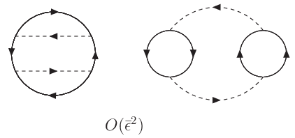
To the next-to-next-to-leading order in $\bar{\epsilon}$ , the pressure receives $O(\bar{\epsilon}^{2})$ corrections from two three-loop diagrams depicted in Fig. 4. The left diagram is easily evaluated as

	$\displaystyle P_{3a}$	$\displaystyle=\left[\bar{g}^{2}\int\!\frac{d{\bm{p}}}{(2\pi)^{d}}\theta(\mu-{\varepsilon_{\bm{p}}})\right]^{2}\int\!\frac{d{\bm{q}}}{(2\pi)^{d}}\delta(\mu-{\varepsilon_{\bm{q}}})$
		$\displaystyle=\frac{\bar{\epsilon}^{2}\mu}{\Gamma\!\left(\frac{d}{2}\right)\Gamma\!\left(\frac{d}{2}+1\right)^{2}}\left(\frac{m\mu}{2\pi}\right)^{d/2}.$		(20)

Now the right diagram in Fig. 4 is written as [29]

\begin{split}P_{3b}&=\bar{g}^{2}\int\!\frac{d{\bm{k}}d{\bm{p}}}{(2\pi)^{2d}}\,\theta(\mu-\varepsilon_{{\bm{p}}+\frac{{\bm{k}}}{2}})\theta(\mu-\varepsilon_{{\bm{p}}-\frac{{\bm{k}}}{2}})\\ &\quad\times\left[1+\bar{g}^{2}\!\int\!\frac{d{\bm{q}}}{(2\pi)^{d}}\frac{\theta(\varepsilon_{{\bm{q}}+\frac{{\bm{k}}}{2}}-\mu)\theta(\varepsilon_{{\bm{q}}-\frac{{\bm{k}}}{2}}-\mu)}{2{\varepsilon_{\bm{q}}}-2{\varepsilon_{\bm{p}}}}\right],\end{split}

(21)

where the frequency integrations are already performed. We note that $+1$ in the square brackets comes from the counter vertex in $\mathcal{L}_{2}$ . Due to the $\theta$ functions, the ranges of integrations over ${\varepsilon_{\bm{k}}}$ , ${\varepsilon_{\bm{p}}}$ , and ${\varepsilon_{\bm{q}}}$ are limited to $0\leq{\varepsilon_{\bm{k}}}\leq 4\mu$ , $0\leq{\varepsilon_{\bm{p}}}\leq\Lambda_{p}$ , and $\Lambda_{q}\leq{\varepsilon_{\bm{q}}}$ , where

\sqrt{\Lambda_{p}}=\frac{-|\cos\chi_{p}|\sqrt{\varepsilon_{\bm{k}}}+\sqrt{4\mu-{\varepsilon_{\bm{k}}}\sin^{2}\chi_{p}}}{2}

(22)

and

\sqrt{\Lambda_{q}}=\frac{|\cos\chi_{q}|\sqrt{\varepsilon_{\bm{k}}}+\sqrt{4\mu-{\varepsilon_{\bm{k}}}\sin^{2}\chi_{q}}}{2},

(23)

with $\cos\chi_{p}=\hat{\bm{k}}\cdot\hat{\bm{p}}$ and $\cos\chi_{q}=\hat{\bm{k}}\cdot\hat{\bm{q}}$ . The integration over ${\varepsilon_{\bm{q}}}$ can be performed analytically using dimensional regularization. As a result, the expression in the square brackets in Eq. (21) becomes

\bigl[\cdots\bigr]=-\frac{\gamma}{2}\bar{\epsilon}-\frac{\bar{\epsilon}}{2}\int_{0}^{\pi}\!\frac{d\chi_{q}}{\pi}\ln\!\left(\frac{\Lambda_{q}-{\varepsilon_{\bm{p}}}}{\mu}\right)+O(\bar{\epsilon}^{2}).

(24)

Then, introducing dimensionless variables $z={\varepsilon_{\bm{k}}}/\mu$ , $\tilde{\Lambda}_{p(q)}=\Lambda_{p(q)}/\mu$ and performing the integration over ${\varepsilon_{\bm{p}}}/\mu$ , we obtain the following expression for $P_{3b}$ :

\begin{split}P_{3b}&=-\bar{\epsilon}^{2}\frac{m\mu^{2}}{2\pi}\biggl[\frac{\gamma}{2}+\frac{1}{2}\int_{0}^{4}\!dz\int_{0}^{\pi}\!\frac{d\chi_{p}}{\pi}\int_{0}^{\pi}\!\frac{d\chi_{q}}{\pi}\\ &\qquad\times\left\{\tilde{\Lambda}_{q}\ln\tilde{\Lambda}_{q}-(\tilde{\Lambda}_{q}-\tilde{\Lambda}_{p})\ln(\tilde{\Lambda}_{q}-\tilde{\Lambda}_{p})-\tilde{\Lambda}_{p}\right\}\biggr].\end{split}

(25)

Finally the numerical integrations over $z$ , $\chi_{p}$ , and $\chi_{q}$ lead to

P_{3b}=-\bar{\epsilon}^{2}\frac{m\mu^{2}}{2\pi}\left(\frac{\gamma}{2}+0.0568528\right)+O(\bar{\epsilon}^{3}).

(26)

Consequently, we obtain the pressure up to the next-to-next-to-leading order in $\bar{\epsilon}$ as

\begin{split}P&=P_{\mathrm{free}}+P_{2}+P_{3a}+P_{3b}\\ &=P_{\mathrm{free}}\left[1+\bar{\epsilon}+0.6931472\,\bar{\epsilon}^{2}+O(\bar{\epsilon}^{3})\right].\end{split}

(27)

The universal parameter of the unitary Fermi gas in Eq. (1) can be equivalently expressed as $\xi_{d}=\mu/\varepsilon_{\mathrm{F}}$ . From the thermodynamic relationship $n=\partial P/\partial\mu$ and the definition of the Fermi energy in $d$ spatial dimensions,

\varepsilon_{\mathrm{F}}=\frac{2\pi}{m}\left[\frac{1}{2}\,\Gamma\!\left(\frac{d}{2}+1\right)n\right]^{2/d},

(28)

we can determine $\xi_{d}$ from the $\bar{\epsilon}$ expansion to be

\begin{split}\xi_{2+\bar{\epsilon}}&=\left[1+\bar{\epsilon}-0.6931472\,\bar{\epsilon}^{2}\right]^{-2/(2+\bar{\epsilon})}\\ &=1-\bar{\epsilon}+0.8068528\,\bar{\epsilon}^{2}+O(\bar{\epsilon}^{3}).\end{split}

(29)

This is the result shown in Eq. (3).

References

[1] For recent reviews, see I. Bloch, J. Dalibard, and W. Zwerger, Rev. Mod. Phys. 80, 885 (2008); S. Giorgini, L. P. Pitaevskii, and S. Stringari, Rev. Mod. Phys. 80, 1215 (2008).
[2] W. Ketterle and M. W. Zwierlein, in Proceedings of the International School of Physics “Enrico Fermi,” Varenna, 2006, edited by M. Inguscio, W. Ketterle, and C. Salomon (IOS Press, Amsterdam, 2008), arXiv:0801.2500, and references therein.
[3] T. Mehen, I. W. Stewart, and M. B. Wise, Phys. Lett. B 474, 145 (2000).
[4] D. T. Son and M. Wingate, Ann. Phys. (N.Y.) 321, 197 (2006).
[5] Y. Nishida and D. T. Son, Phys. Rev. D 76, 086004 (2007).
[6] T. Mehen, Phys. Rev. A 78, 013614 (2008).
[7] K. M. O’Hara et al., Science 298, 2179 (2002).
[8] M. Bartenstein et al., Phys. Rev. Lett. 92, 120401 (2004).
[9] T. Bourdel et al., Phys. Rev. Lett. 93, 050401 (2004).
[10] J. Kinast et al., Science 307, 1296 (2005).
[11] G. B. Partridge et al., Science 311, 503 (2006).
[12] J. T. Stewart et al., Phys. Rev. Lett. 97, 220406 (2006).
[13] L. Tarruell et al., arXiv:cond-mat/0701181.
[14] J. Carlson, S.-Y. Chang, V. R. Pandharipande, and K. E. Schmidt, Phys. Rev. Lett. 91, 050401 (2003).
[15] S. Y. Chang, V. R. Pandharipande, J. Carlson, and K. E. Schmidt, Phys. Rev. A 70, 043602 (2004).
[16] G. E. Astrakharchik, J. Boronat, J. Casulleras, and S. Giorgini, Phys. Rev. Lett. 93, 200404 (2004).
[17] J. Carlson and S. Reddy, Phys. Rev. Lett. 95, 060401 (2005).
[18] A. Bulgac, J. E. Drut, and P. Magierski, Phys. Rev. Lett. 96, 090404 (2006).
[19] D. Lee, Phys. Rev. B 73, 115112 (2006).
[20] T. Abe and R. Seki, arXiv:0708.2524.
[21] A. Bulgac, J. E. Drut, P. Magierski, and G. Wlazlowski, arXiv:0801.1504.
[22] D. Lee, Phys. Rev. C 78, 024001 (2008).
[23] S. Zhang, K. E. Schmidt, and J. Carlson, unpublished.
[24] Y. Nishida and D. T. Son, Phys. Rev. Lett. 97, 050403 (2006).
[25] Y. Nishida and D. T. Son, Phys. Rev. A 75, 063617 (2007).
[26] Y. Nishida, Phys. Rev. A 75, 063618 (2007).
[27] Z. Nussinov and S. Nussinov, Phys. Rev. A 74, 053622 (2006).
[28] P. Arnold, J. E. Drut, and D. T. Son, Phys. Rev. A 75, 043605 (2007).
[29] Y. Nishida, Ph. D. Thesis, University of Tokyo, 2007 [available as arXiv:cond-mat/0703465]. For the NNLO correction near $d=2$ , see also the Appendix of the current paper.
[30] G. Rupak, arXiv:nucl-th/0605074.
[31] G. Rupak, T. Schafer, and A. Kryjevski, Phys. Rev. A 75, 023606 (2007).
[32] J. W. Chen and E. Nakano, Phys. Rev. A 75, 043620 (2007).
[33] A. Kryjevski, Phys. Rev. A 78, 043610 (2008); arXiv:0804.2919.
[34] G. Rupak and T. Schafer, Nucl. Phys. A816, 52 (2009).

Ground-state energy of the unitary Fermi gas from the ϵ\epsilon expansion