KBSM of the product of a disk with two holes and $S^{1}$

Skein modules, as invariants of $3$-manifolds, were introduced by J. Przytycki [7] and V. Turaev [9] in 1987 and have become important algebraic structures for studying $3$-dimensional manifolds $M^{3}$ and knot theory in $M^{3}$. The Kauffman Bracket Skein Module (KBSM) is the most extensively studied skein module. We recall its definition here for the purposes of further sections.

The local relations are the ones that arise in the definition of the Kauffman bracket polynomial of a link. By local relations we mean that the three links $L_{+}$, $L_{-}$, and $L_{\infty}$ are three framed links that are identical outside some small neighborhood. It can quickly be seen that $L^{(1)}=-A^{3}L$ (where $L^{(1)}$ is $L$ with a positive twist) in $\mathcal{S}_{2,\infty}(M^{3};R,A)$ which we call the framing relation.

As it was shown in [8] and [4] $\mathcal{S}_{2,\infty}(S^{3};R,A)$ is free cyclic, $\mathcal{S}_{2,\infty}(S^{1}\times I\times I;R,A)$ and $\mathcal{S}_{2,\infty}(S^{1}\times S^{1}\times I;R,A)$ are free modules, generated by infinite sets, whereas $\mathcal{S}_{2,\infty}(S^{2}\times S^{1};R,A)$ has torsion. However, the KBSM has been found for considerably large classes of $3$ - dimensional manifolds [8, 4, 2, 3, 1], and the following problem was proposed in [6] (see Problem $4.4$, pp. 446): Find KBSM of the $3$- manifold that is obtained as the product of a disk with two holes and $S^{1}$. Let $F_{g,k}$ denote an orientable surface of genus $g$ with $k$ boundary components. In this paper, we compute $S_{2,\infty}(F\times S^{1};R,A)$, where $F$ is a disk $D^{2}=F_{0,1}$, annulus $A=F_{0,2}$, and disk with two holes $F_{0,3}$. The modules $S_{2,\infty}(F\times S^{1};R,A)$ for $F=D^{2}$ and $F=F_{0,2}$ were shown to be free in [8], however the methods developed for computing them will be used in our latter computations of $S_{2,\infty}(F_{0,3}\times S^{1};R,A).$ Our main result (see Theorem 5.3) stating, that $S_{2,\infty}(F_{0,3}\times S^{1};R,A)$ is free solves, in particular, the Problem $4.4$ of J. Przytycki ([6], pp. 447) and supports the conjecture (see Conjecture $4.3$, [6], pp. 446) that if every closed incompressible surface in $M^{3}$ is parallel to the boundary of the $3$-manifold $\partial M^{3}$ then $S_{2,\infty}(M^{3};R,A)$ of $M^{3}$ is torsion free¹¹ 1 As it was shown in [4] and [10] incompressible (non-boundary parallel) surface can cause torsion in KBSM . Therefore, our result concerning $S_{2,\infty}(F_{0,3}\times S^{1},\mathbb{Z}\left[A^{\pm 1}\right],A)$ also suggests that torsion in the KBSM cannot be caused by the existence of an immersed torus..

Let $F$ be an orientable surface (possibly with boundary) and $I=[0,1]$. Let $f:F\times I\rightarrow F\times S^{1}$ be given by $f(x,y)=(x,$ $e^{2\pi iy})$. Using an argument of general position we can assume that all links $L$ in $F\times S^{1}$ are transversal to $F\times\{1\}$. Then each $f^{-1}(L)$ consists of embedded arcs in $F\times I$ with all endpoints coming in pairs of the form $\{(x,0),(x,1)\}$ where $x\in F$.

Let $p$ denote the projection of $F\times I$ onto $F\times\{0\}=F$, given by $p(x,y)=(x,0)$. If $D=p(f^{-1}(L))$ then $D$ consists of immersed curves in $F$. A point in $D$ that corresponds to a pair of endpoints of $f^{-1}(L)$ is called a dot in $D$. Again, applying an argument of general position, we may assume that all dots in $D$ are distinct and that there are only transversal double points in $D$ that are disjoint from dots. Near each of the double points of $D$ we label two branches as upper and lower according to their corresponding values of the arguments $y$ in the second coordinate. Moreover, while the link $L$ crosses the surface $f\left(F\times\{1\}\right)=f\left(F\times\{0\}\right)$ (near the point $(x_{0},1)\in F\times S^{1}$ of the intersection) the corresponding arc component containing $(x_{0},1)\in F\times I$ has the $y$ values close to $1$ and increasing in coordinate $y$. Therefore, the corresponding dot in $D$ is passed in the unique direction (determined by the increasing values of $y)$. Hence, each link in $F\times S^{1}$ determines uniquely an assignment of arrows at dots in $D$. Now, a diagram of $L$ in $F\times S^{1}$ consists of $D$ together with additional information regarding over and under branches (for double points of $D$) and an assignment of arrows (for dots in $D$). An example, showing the construction of the diagram of a link $L$ in $F_{0,3}\times S^{1}$ is shown in Figure 2.1.

Two links in $F\times S^{1}$ are isotopic if their diagrams differ by a finite sequence of ”Reidemeister moves”. These moves are obtained while we consider the resolution of generic singularities for the diagrams: cusps, tangency points, and triple points give us the classical Reidemeister moves $\Omega_{1}$, $\Omega_{2}$ and $\Omega_{3}$; double dots give us the fourth move $\Omega_{4}$; and dots combined with double points give us the fifth move $\Omega_{5}$. All moves are shown in Figure 2.2. The geometric interpretation for the $\Omega_{4}$ and $\Omega_{5}$-moves is shown in Figure 2.3. We call the moves $\Omega_{2}$, $\Omega_{3},$ $\Omega_{4},$ and $\Omega_{5}$ regular Reidemeister moves²² 2 Analogy with the classical case of links in $S^{3}.$.

Let $L$ be a link in $S^{1}\times D^{2}$ and $D$ its diagram. Each double point of $D$ (crossing of $D$) can be equipped with a positive or a negative marker corresponding to the horizontal and vertical smoothings.

A state $s$ of the diagram $D$ is the choice of a marker for each crossing of $D$. Let $p(s)$ (resp. $n(s)$) be the number of crossings with positive (resp. negative) markers in $s$. Let $D(s)$ be the diagram obtained from $D$ by smoothing all crossings in $D$ according to the markers determined by $s$ and removing all pairs of opposite arrows by the $\Omega_{4}$-move. To each component of $D(s)$ is assigned an integer that gives the number of arrows on this component (arrows giving the counterclockwise orientation of the component are counted as positive, and those giving the clockwise orientation are counted as negative) as shown in Figure 3.2. We will refer to such a component as component with $n$ arrows.

A component $c$ of $D(s)$ is called trivial if there are no arrows on it and every connected component lying inside the disk bounded by $c$ also has no arrows. Let us denote by $|s|$ the number of trivial components of $D(s)$ and by $D^{\prime}(s)$ the diagram obtained from $D(s)$ by removing all trivial components.

Proof. The proof for the invariance of the bracket $\left\langle\hskip 5.69046pt\right\rangle$ under $\Omega_{2}$ and $\Omega_{3}$-moves is analogous to the classical case $($Kauffman bracket for classical diagrams [5]$),$ and invariance of $\left\langle\hskip 5.69046pt\right\rangle$ under $\Omega_{4}$-move follows directly from its definition.  

The invariance of $\left\langle\hskip 5.69046pt\right\rangle$ under the $\Omega_{5}$-move requires more detailed analysis. For this reason, we first introduce a ”refined version” of the bracket which is unchanged under the $\Omega_{5}$-move. Let us denote by $x$ the diagram and by $\mathbb{N}=\{0,$ $1,$ $2,...\}$ the set of all natural numbers. We show that the $S_{2,\infty}(D^{2}\times S^{1};R,A)$ is a free $R$-module, generated by $\{x^{n}\mid n\in\mathbb{N}\}$, where $x^{n}$ stands for ($n$ copies of $x,$ and $x^{0}=\emptyset$).

Proof. Using the fact that the removal of a positive kink contributes $-A^{3}$ in the KBSM, and the removal of a negative kink contributes $-A^{-3}$ (just as it is for the classical case of the Kauffman bracket [5]), we have:

$$\psfig{file={figxinv.eps},scale={0.25}}=-A^{-3}\psfig{file={figxinvkink.eps},scale={0.55}}=-A^{-3}\psfig{file={figxinvkinkcrch.eps},scale={0.3}}=A^{-6}\psfig{file={figx.eps},scale={0.25}}.$$

The above calculation finishes our argument.  

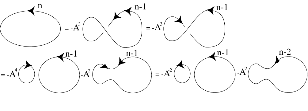
Let $D_{n}$ be the diagram that consists of a single component with no crossings and $n$ arrows. Using the calculation shown in Figure 3.3 and applying Lemma 3.3, we can express $D_{n}$ in $S_{2,\infty}(D^{2}\times S^{1};R,A)$ as the combination of $D_{n-1}$ and $D_{n-2}$. Therefore, the following recursion holds true in $S_{2,\infty}(D^{2}\times S^{1};R,A)$:

Let $D_{n,k}$ be the diagram with no crossings and consisting of $k+1$ components, where $k$ of these components (corresponding to $x^{k})$ are encircled by a single component with $n$ arrows. We show in Figure 3.4 how to express $D_{n,k}$ as a combination of $D_{n+1,k-1}$ and $D_{n,k-1}$. Hence, the following recursion holds true in $S_{2,\infty}(D^{2}\times S^{1};R,A)$:

The recursive relations 3.1 and 3.2 motivate the following definition.

We have for instance that $P_{-1}=A^{-6}x$. Now we are ready to define the refined Kauffman bracket.

We notice that the refined Kauffman bracket was defined in such a way that it clearly satisfies relations 3.1 and 3.2. Therefore, we have the following identities:

It also follows from the definition that for the refined bracket $\left\langle\hskip 5.69046pt\right\rangle_{r}$, the above two relations hold true even when they occur in a disk outside of which there are components which are not involved in the three diagrams appearing in the relations. We show that $\left\langle\hskip 5.69046pt\right\rangle_{r}$ satisfies a generalized version of the relation 3.1.

Let $D_{r}$, $D_{l}$, $D_{u}$, and $D_{d}$ be four diagrams which are the same outside a small disk but which differ inside the disk as it is shown in Figure 3.5.

Proof. We observe that it suffices to prove $(1)$ and $(2)$ for diagrams with no crossings and no trivial components. In $D^{\prime}(s)$ let us consider only the components of $D^{\prime}(s)$ that are inside the component $C$ to which the vertical segment shown in Figure 3.5 belongs. Suppose that $\left\langle\hskip 5.69046pt\right\rangle_{r}$ is applied to these components so that they are replaced by the linear combination of $x^{k}$’s (polynomials in $x$). Therefore, it suffices to prove $(1)$ and $(2)$ in the case when there is only one $x^{k}$ inside $C$.

$(1)$ First, let us assume that in $D_{r}$ the circle $x$ is outside relative to the component $C$. When computing $\left\langle\hskip 5.69046pt\right\rangle_{r}$ any circles inside $C$ are first pushed outside using the relation 3.2. This modifies $D_{u}$, $D_{r}$ and $D_{d}$ in the same way and by the same linear combinations. Thus, we can assume that there are no $x$-components inside $C$. Considering only $C$ and the circles appearing in Figure 3.5 (since contribution of the others is the same when computing $\left\langle\hskip 5.69046pt\right\rangle_{r}$), we notice that

Since the refined bracket $\left\langle\hskip 5.69046pt\right\rangle_{r}$ satisfies relation 3.1, we have:

which gives $(1)$.

Suppose now that in $D_{r}$ the circle $x$ is inside relative to $C$. As before, when computing $\left\langle\hskip 5.69046pt\right\rangle_{r}$, one pushes the $x$’s out of $C$ except for the circle in $D_{r}$. In this case we observe that:

Relation 3.2 for $\left\langle\hskip 5.69046pt\right\rangle_{r}$ gives:

which is equivalent to:

Since $\left\langle\hskip 5.69046pt\right\rangle_{r}$ satisfies relation 3.1, we also have:

which, in turn, is equivalent to:

In the last equation, substituting for $-A^{-4}\left\langle D_{l}\right\rangle_{r}$ from the equation before, we obtain:

which proves the identity $(1).$

$(2)$ From part $(1)$ one has

which is equivalent to:

Now, we observe that after rotating the diagrams in Figure 3.5 by $\pi$, we have $D_{u}$ is switched with $D_{d}$ and $D_{r}$ is switched with $D_{l}$. Relabelling them accordingly in the last equation gives $(2)$.  

Proof. By the result of Lemma 3.2, the Kauffman bracket $\left\langle\hskip 5.69046pt\right\rangle$ is preserved by $\Omega_{2},$ $\Omega_{3},$ and $\Omega_{4}$-moves, thus the same holds true for the refined Kauffman bracket $\left\langle\hskip 5.69046pt\right\rangle_{r}$. It remains to study the case when diagrams $D$ and $D^{\prime}$ differ by an $\Omega_{5}$ -move. We may assume that there is only one crossing in these diagrams, with all others being smoothed using the relation $(K1)$. Moreover, we may assume that inside the disks bounded by the component with the crossing all other components are already expressed as polynomials in $x$. Moreover, as the contribution of components outside the component (on which the move is performed) is the same for both $D$ and $D^{\prime}$, we can additionally assume that there are no such components. Thus, we need to check the invariance of $\left\langle\hskip 5.69046pt\right\rangle_{r}$ in the two cases shown in Figures 3.6 and 3.7.

In Figure 3.6 one needs to verify that $\left\langle D\right\rangle_{r}=\left\langle D^{\prime}\right\rangle_{r}$. Applying Lemma 3.6 for $D$ and $D^{\prime}$, one pushes the $x$’s in the parts with $m$ arrows (at the expense of getting diagrams with $m+1$ and $m-1$ arrows). Analogously, the same happens for the part with $n$ arrows. Therefore, it is sufficient to check the case when $k=0$ and $l=0$. Now, applying Lemma 3.6 again for both diagrams, one may push out an arrow from the part with $n$ arrows, at the expense of some exterior $x$ and diagrams with $n-1$ and $n-2$ arrows. Thus, it is sufficient to prove the case for $n=0$ and $n=1$ (one may also reduce $m$ to $0$ or $1$ however, for our proof it is not needed).

For $n=0$, we have:

and using the inductive definition of $P_{n}$ we have:

In the case shown in Figure 3.7, we also use similar reasoning as in $(1)$ to reduce it to the case when we can assume that $l=0$ and $k=0$ (applying Lemma 3.6). Then again, we apply Lemma 3.6 to push out all the arrows, we arrive again at the situation when it is sufficient to consider the cases $n=0$ and $n=-1$. We discuss each one of these cases below.

For $n=0$, we have:

and using inductive definitions of $P_{n}$ and $P_{n,k}$ we obtain:

Let $A=F_{0,2}$ denote an annulus. The Kauffman bracket for diagrams of links in $A\times S^{1}$ is defined in a way that is analogous to the previous case (see Definition 3.1). However, we notice that after smoothing all of the crossings in such a diagram, there are now two types of components: ones bounding a disk (called the $x$-type) or ones parallel to the boundary $\partial A=S^{1}\sqcup S^{1}$ components (called the $y$-type).

The Kauffman bracket is first refined in the way analogous to the one introduced in Definition 3.5. Using the refined bracket for the $x$-type components enclosed between two successive components of the $y$-type allows us to express the $x$-type components as linear combinations of $x^{n}$ $(n\geq 0)$ over $R$. Thus, the refined bracket $\left\langle D\right\rangle_{r}$ for the diagram $D$ can be written as a linear combination of diagrams shown in Figure 4.1. Moreover, an order of the two boundary components in $\partial A$ induces a natural order of the $y$-type components and all terms $x^{n}$ enclosed by any two successive $y$-type components. We use the ordering from the ”interior” $S^{1}$ to the ”exterior” $S^{1}$ of $\partial A$ for all of our diagrams. Therefore, diagrams that constitute terms of the polynomial $\left\langle D\right\rangle_{r}$ can be encoded uniquely by words of the form

Every word $w=y_{m_{1}}y_{m_{2}}...y_{m_{k}}x^{n},$ where $m_{i}=0$ or $1;$ $n\in\mathbb{N}$ will be called semi-reduced. For a given word $w$ we define inductively the semi-reduced refined bracket $\left\langle w\right\rangle_{srr}$ corresponding to the diagram of $w$, as a linear combination of semi-reduced words.

$(1)$ If $w$ is semi-reduced, we set $\left\langle w\right\rangle_{srr}=w$.

If $w$ is not semi-reduced then $w$ contains the letter $x$ before some $y_{n}$ or the letter $y_{n}$ where $n\in\mathbb{Z}\backslash\{0,1\}$. We write $w=w_{1}w_{2},$ where $w_{1}$ is semi-reduced and contains no $x$.

$(2)$ If $w_{2}$ starts with the letter $x$ then $w_{2}=x^{k}y_{n}w_{3}$ for some word $w_{3}$. Using the calculation shown in Figure 3.4, we obtain the following relation in the KBSM:

and in this case we define

$(3)$ If $w_{2}$ starts with $y_{n}$, where $n>1$ (that is, $w_{2}=y_{n}w_{3}$ for some word $w_{3}$), using the calculation shown in Figure 3.3 we obtain the following relation in the KBSM:

and accordingly, we define

$(4)$ If $n<0$ then the last relation is used to express the word containing $y_{n}$ with words containing $y_{n+1}$ and $y_{n+2}$ and we define $\left\langle w\right\rangle_{srr}$ accordingly.

It can easily be seen that the inductive definition of $\left\langle w\right\rangle_{srr}$ results with a linear combination of semi-reduced words.

Now, we prove another generalized version of Lemma 3.6.

Proof. If the vertical segment shown in Figure 3.5 is a part of the $x$-type component, then the proof is the same as for the Lemma 3.6 and, moreover, the identities $(1)$ and $(2)$ hold true even for the refined Kauffman bracket $\left\langle\hskip 5.69046pt\right\rangle_{r}$. For the other case (when the vertical line segment is a part of the $y$-type component) we observe, as before in the proof of Lemma 3.6, that the relations 3.1 and 3.2 hold true for $\left\langle\hskip 5.69046pt\right\rangle_{srr}$, where instead of $D_{n}$ we take $y_{n}$, and any configuration of the remaining components. Indeed, the components between the first boundary component $S^{1}$ of $\partial A$ and $y_{n}$ are reduced while computing $\left\langle\hskip 5.69046pt\right\rangle_{srr}$ to a point when there is some $x^{k}$ to be pushed through the $y_{n}$. The rest of the proof is the same as for Lemma 3.6: one pushes all $x$’s, or all but one, through $y_{n}$, and then $(1)$ follows from definition of $\left\langle\hskip 5.69046pt\right\rangle_{srr}$. The property $(2)$ is a consequence of $(1)$ exactly for the same reasons as in the proof of Lemma 3.6.  

Since the Kauffman bracket $\left\langle\hskip 5.69046pt\right\rangle$ is invariant under $\Omega_{2}$, $\Omega_{3},$ and $\Omega_{4}$-moves it follows that the same is true for all other brackets we defined. To check the invariance of $\left\langle\hskip 5.69046pt\right\rangle_{srr}$ under the $\Omega_{5}$-move one may, as before, consider diagrams where all crossings are smoothed except for the crossing directly involved in the move. In $S^{1}\times A$ we have five versions (types) of such moves shown in Figure 4.2, where only the first boundary component $S^{1}$ of $\partial A$ is shown and, instead of presenting the actual $\Omega_{5}$-move, we show only the type of a component on which this move is performed.

For the moves of type $\mathbf{I}$ and $\mathbf{II}$ shown in Figure 4.2 (where smoothing in both ways gives components bounding disks in $A\,$) $\left\langle\hskip 5.69046pt\right\rangle_{r}$ is invariant by Proposition 3.7 and therefore the same holds true for $\left\langle\hskip 5.69046pt\right\rangle_{srr}$ and $\left\langle\hskip 5.69046pt\right\rangle_{rr},$ where $\left\langle\hskip 5.69046pt\right\rangle_{rr}$ is defined after the proof of Proposition 4.3 (see Definition 4.4).

Proof. For the move of type $\mathbf{III}$ the situation is shown in Figure 4.3. We may assume that $\left\langle\hskip 5.69046pt\right\rangle_{srr}$ is applied locally inside of the disks and annuli that are introduced later after all crossings are smoothed. Applying Lemma 4.2, we can push all the components $x^{k}$ outside of the component on which the $\Omega_{5}$-move is applied and then, using the same lemma again, we can also reduce $n$ to $0$ or $1$. Moreover, we can disregard all the components inside and outside the component on which $\Omega_{5}$-move is applied (see Figure 4.3) since they equally contribute to $\left\langle D\right\rangle_{srr}$ and $\left\langle D^{\prime}\right\rangle_{srr}$.

For $n=0$, smoothing both sides gives the following relation

which, after multiplying by $-A^{3}$ gives the relation 3.1 which holds for $\left\langle\hskip 5.69046pt\right\rangle_{srr}$.

For $n=1$, we have:

which, after multiplying by $A^{-1}$ becomes again the relation 3.1 which holds for $\left\langle\hskip 5.69046pt\right\rangle_{srr}$.

For type $\mathbf{IV}$ the situation is presented in Figure 4.4.

As in the previous case, we reduce $n$ to $0$ or $-1$ and disregard all components except the one on which the $\Omega_{5}$-move is applied. We consider again both cases below.

For $n=0$, after smoothing the crossing in $D^{\prime}$ and an application of relations 3.2 and 3.1, which hold for $\left\langle\hskip 5.69046pt\right\rangle_{srr}$, we obtain

which is the same as the result of the smoothing of the crossing in $D$.

For $n=-1$, smoothing the crossing in $D$ and using relations 3.2 and 3.1, which hold for $\left\langle\hskip 5.69046pt\right\rangle_{srr}$, gives

which is the same as the result of smoothing of the crossing in $D^{\prime}$.  

In order to show the invariance under the $\Omega_{5}$-move of all five types shown in Figure 4.2, we need another refinement where the semi-reduced words are expressed as the reduced words or words of the form $y_{m_{1}}y_{m_{2}}...y_{m_{k+1}}x^{n}$, where the $m_{1}=m_{2}=...=m_{k}=0$, and $m_{k+1}$ is $0$ or $1$, $n\in\mathbb{N}$. To simplify our notations we set $y_{0}=y$ and $y_{1}=y^{\prime},$ thus the reduced words have the form $y^{k}x^{n}$ or $y^{k}y^{\prime}x^{n}$. Let $w$ be a semi-reduced word (and at the same time the diagram represented by this word). We define inductively the reduced refinement $\left\langle w\right\rangle_{rr}$ as a linear combination of reduced words.

$(1)$ If $w$ is reduced, we set $\left\langle w\right\rangle_{rr}=w$.

Otherwise $w$ must contain a subword of the form $y^{\prime}y$ or $y^{\prime}y^{\prime}$.

$(2)$ Suppose that $w=y^{k}y^{\prime}yw_{2}$. In the KBSM the word $w$ satisfies the following relation:

References

• [1] D. Bullock, On the Kauffman bracket skein module of surgery on a trefoil, Pacific J. Math. 178 (1997), No. 1, pp. 37-51.
• [2] J. Hoste, J. H. Przytycki, Homotopy skein modules of oriented 33-manifolds, Math. Proc. Cambridge Phil. Soc. 108 (1990), pp. 475-488.
• [3] J. Hoste, J. H. Przytycki, The skein module of genus 11 Whitehead type manifolds, Journal of Knot Theory with Its Ramifications 4 (1995), No. 3, pp. 411-427.
• [4] J. Hoste, J. H. Przytcki, The Kauffman bracket skein module of S1×S2S^{1}\times S^{2}, Math. Z. 220 (1995), No. 1, pp. 63-73.
• [5] L. H. Kauffman, State models and the Jones polynomial, Topology 26 (1987), No. 3, pp. 395-407.
• [6] T Ohtsuki (editor), Problems on invariants of knots and 3-manifolds, Geometry & Topology Monographs 4 (2002), pp. 377-572.
• [7] J. H. Przytycki, Skein modules of 3-manifolds. Bull. Polish Acad. Sci. 39 (1991), No. 1-2, pp. 91-100.
• [8] J. H. Przytycki, Fundamentals of Kauffman bracket skein modules, Kobe J. Math. 16 (1999), No. 1, pp. 45–66.
• [9] V. G. Turaev, The Conway and Kauffman modules of a solid torus, J. Soviet Math. 52 (1990), pp. 2799-2805.
• [10] M. A. Veve, Torsion in the KBSM of a 33-manifold caused by an incompressible torus and detected by a complete hyperbolic structure, Kobe Journal of Mathematics 16 (1999), No. 2, pp. 109-118.