跳到论文正文
W Papers独立论文阅读器 arXiv:0808.3731 论文正文 计算阅读时间 · 0%
引用这篇论文根据当前论文元数据生成,正式投稿前建议核对。


License: arXiv.org perpetual non-exclusive license
arXiv:0808.3731v3 [hep-ph] 16 Sep 2008

K𝟏​(𝟏𝟐𝟕𝟎)K_{1}(1270)–K𝟏​(𝟏𝟒𝟎𝟎)K_{1}(1400) Mixing Angle and New-Physics Effects in B→K𝟏​ℓ+​ℓ−B\to K_{1}\ell^{+}\ell^{-} Decays

Hisaki Hatanaka Affiliation: Department of Physics, Chung-Yuan Christian University, Chungli 320, Taiwan    Kwei-Chou Yang Affiliation: Department of Physics, Chung-Yuan Christian University, Chungli 320, Taiwan
Abstract

We study semileptonic BB meson decays B→K1​(1270)​ℓ+​ℓ−B\to K_{1}(1270)\ell^{+}\ell^{-} and K1​(1400)​ℓ+​ℓ−K_{1}(1400)\ell^{+}\ell^{-} (ℓ≡e\ell\equiv e, μ\mu, τ\tau), where the strange PP-wave mesons, K1​(1270)K_{1}(1270) and K1​(1400)K_{1}(1400), are the mixtures of the K1​AK_{1A} and K1​BK_{1B}, which are the 13​P11^{3}P_{1} and 11​P11^{1}P_{1} states, respectively. We show that the ratio Rℓ≡ℬ⁡(B→K1​(1400)​ℓ+​ℓ−)/ℬ⁡(B→K1​(1270)​ℓ+​ℓ−)R_{\ell}\equiv{\cal B}(B\to K_{1}(1400)\ell^{+}\ell^{-})/{\cal B}(B\to K_{1}(1270)\ell^{+}\ell^{-}), insensitive to new-physics parameters, is suitable for determining the K1​(1270)K_{1}(1270)–K1​(1400)K_{1}(1400) mixing angle, θK1\theta_{K_{1}}. The forward-backward asymmetry shows a weak θK1\theta_{K_{1}}-dependence for B→K1​(1270)​μ+​μ−B\to K_{1}(1270)\mu^{+}\mu^{-}, but relatively strong for B→K1​(1400)​μ+​μ−B\to K_{1}(1400)\mu^{+}\mu^{-}. We investigate model-independent new-physics corrections to operators relevant to the b→s​ℓ+​ℓ−b\to s\ell^{+}\ell^{-} electroweak-penguin and weak-box diagrams. Furthermore, for the B→K1​(1270)​μ+​μ−B\to K_{1}(1270)\mu^{+}\mu^{-} decay the position of the forward-backward asymmetry zero, which is almost independent of the value of θK1\theta_{K_{1}}, can be dramatically changed under variation of new-physics parameters.

pacs
13.20.He, 14.40.Ev, 13.20.-v,12.60.-i

I Introduction

Table 1: Experimental status of branching fractions (in units of 10−610^{-6}) for the decays B→K∗​(892)​γB\to K^{*}(892)\gamma, K1​(1270)​γ,K1​(1400)​γK_{1}(1270)\gamma,K_{1}(1400)\gamma and B→K∗​(892)​ℓ+​ℓ−B\to K^{*}(892)\ell^{+}\ell^{-} [1].
Mode Exp.(Average) Ref. Mode Exp.(Average) Ref.
K∗⁣+​(892)​γK^{*+}(892)\gamma 40.3±2.640.3\pm 2.6 [2, 3, 4] K∗0​(892)​γK^{*0}(892)\gamma 40.1±2.040.1\pm 2.0 [2, 3, 4]
K1+​(1270)​γK_{1}^{+}(1270)\gamma 43±1243\pm 12 [5] K10​(1270)​γK_{1}^{0}(1270)\gamma <58<58 [5]
K1+​(1400)​γK_{1}^{+}(1400)\gamma <15<15 [5] K10​(1400)​γK_{1}^{0}(1400)\gamma <15<15 [5]
K∗⁣+​(892)​e+​e−K^{*+}(892)e^{+}e^{-} 1.23−0.62+0.691.23^{+0.69}_{-0.62} [6, 7] K∗0​(892)​e+​e−K^{*0}(892)e^{+}e^{-} 1.11−0.26+0.301.11^{+0.30}_{-0.26} [6, 7]
K∗⁣+​(892)​μ+​μ−K^{*+}(892)\mu^{+}\mu^{-} 0.78−0.44+0.560.78^{+0.56}_{-0.44} [6, 7] K∗0​(892)​μ+​μ−K^{*0}(892)\mu^{+}\mu^{-} 0.98−0.21+0.220.98^{+0.22}_{-0.21} [6, 7]

b→sb\to s transitions in semileptonic and radiative BB meson decays contain rich phenomena relevant to the standard model (SM) and new physics (NP). Semileptonic and radiative BB decays involving a vector or axial vector meson have been observed by BABAR, Belle and CLEO (see Table 1). The rare flavor-changing neutral-current processes, b→s​ℓ¯​ℓb\to s\bar{\ell}\ell, which proceed through the electroweak-penguin and weak-box diagrams in the SM, may provide a hunting ground to search for the NP effects. For B→K∗​(892)​ℓ+​ℓ−B\to K^{*}(892)\ell^{+}\ell^{-} decays, the forward-backward asymmetry has been measured by BABAR [7] and Belle [8]. Very recently, BABAR [9, 10, 11] has reported the measurements for the longitudinal polarization fraction and forward-backward asymmetry (FBA) of B→K∗​(892)​ℓ+​ℓ−B\to K^{*}(892)\ell^{+}\ell^{-}, and for the isospin asymmetry of B0→K∗0​(892)​ℓ+​ℓ−B^{0}\to K^{*0}(892)\ell^{+}\ell^{-} and B±→K∗⁣±​(892)​ℓ+​ℓ−B^{\pm}\to K^{*\pm}(892)\ell^{+}\ell^{-} channels. The data may hint at the flipped sign(s) of the Wilson coefficients, e.g., the flipped sign of c7effc^{\rm eff}_{7} related to the magnetic dipole operator. To extract the moduli and arguments of the effective Wilson coefficients, it is important to measure various observables in different inclusive and exclusive rare processes. These should be considerably improved at LHCb.

The radiative BB decay involving the K1​(1270)K_{1}(1270), the orbitally excited (PP-wave) state, is recently observed by Belle and other radiative and semileptonic decay modes involving K1​(1270)K_{1}(1270) and K1​(1400)K_{1}(1400) are hopefully expected to be seen soon. Some studies for B→K1​ℓ+​ℓ−B\to{K_{1}}\ell^{+}\ell^{-} have been made recently [12, 13, 14]. Just like B→K∗​(892)​ℓ+​ℓ−B\to K^{*}(892)\ell^{+}\ell^{-} decays [15, 17, 16, 18, 19, 20, 21, 22], B→K1​ℓ+​ℓ−B\to{K_{1}}\ell^{+}\ell^{-} decays can offer the good probe to the NP, and are much more sophisticated due to the mixing of the K1​AK_{1A} and K1​BK_{1B}, which are the 13​P1{1^{3}P_{1}} and 11​P1{1^{1}P_{1}} states, respectively. The physical K1K_{1} mesons are K1​(1270)K_{1}(1270) and K1​(1400)K_{1}(1400), described by

(|K¯1​(1270)⟩|K¯1​(1400)⟩)=M​(|K¯1​A⟩|K¯1​B⟩),withM=(sin⁡θK1cos⁡θK1cos⁡θK1−sin⁡θK1).\displaystyle\pmatrix{|\overline{K}_{1}(1270)\rangle\cr|\overline{K}_{1}(1400)\rangle}=M\pmatrix{|\overline{K}_{1A}\rangle\cr|\overline{K}_{1B}\rangle},\quad\mbox{with}\quad M=\pmatrix{\sin\theta_{K_{1}}&\phantom{-}\cos\theta_{K_{1}}\cr\cos\theta_{K_{1}}&-\sin\theta_{K_{1}}}. (1)

The magnitude of θK1\theta_{K_{1}} was estimated to be |θK1|≈34∘∨57∘|\theta_{K_{1}}|\approx 34^{\circ}\vee 57^{\circ} in Ref. [23], 35∘≲|θK1|≲55∘35^{\circ}\lesssim|\theta_{K_{1}}|\lesssim 55^{\circ} in Ref. [24], and |θK1|=37∘∨58∘|\theta_{K_{1}}|=37^{\circ}\vee 58^{\circ} in Ref. [25]. Nevertheless, the sign of the θK1\theta_{K_{1}} was not yet determined in these studies. From the study for B→K1​(1270)​γB\to K_{1}(1270)\gamma and τ→K1​(1270)​ντ\tau\to K_{1}(1270)\nu_{\tau}, we recently obtain [26]

θK1=−(34±13)∘,\displaystyle\theta_{K_{1}}=-(34\pm 13)^{\circ}, (2)

where the minus sign of θK1\theta_{K_{1}} is related to the chosen phase of |K¯1​A⟩|{\overline{K}_{1A}}\rangle and |K¯1​B⟩|{\overline{K}_{1B}}\rangle. We adopt the following conventions [26]: fK1​A>0f_{K_{1A}}>0 and fK1​B⟂>0f_{K_{1B}}^{\perp}>0, which are defined by

⟨0​|ψ¯​γμ​γ5​s|​K¯1​A​(P,λ)⟩\displaystyle\langle{0}|\bar{\psi}\gamma^{\mu}\gamma_{5}s|{\overline{K}_{1A}(P,\lambda)}\rangle =\displaystyle= −i​fK1​A​mK1​A​εμ(λ),\displaystyle-if_{K_{1A}}m_{K_{1A}}\varepsilon_{\mu}^{(\lambda)},
⟨0​|ψ¯​σμ​ν​s|​K¯1​B​(P,λ)⟩\displaystyle\langle{0}|\bar{\psi}\sigma_{\mu\nu}s|{\overline{K}_{1B}(P,\lambda)}\rangle =\displaystyle= i​fK1​B⟂​ϵμ​ν​α​β​ε(λ)α​Pβ,ψ≡d,u.\displaystyle if^{\perp}_{K_{1B}}\epsilon_{\mu\nu\alpha\beta}\varepsilon_{(\lambda)}^{\alpha}P^{\beta},\quad\psi\equiv d,u. (3)

Within the SM, we have predicted [26]

ℬ⁡(B−→K1−​(1270)​γ)\displaystyle{\cal B}(B^{-}\to K_{1}^{-}(1270)\gamma) =\displaystyle= (66−30+50)×10−6​(mb.p​o​l​e4.90​GeV)2,\displaystyle(66^{+50}_{-30})\times 10^{-6}\left(\frac{m_{b.pole}}{4.90~{\rm GeV}}\right)^{2}~, (4)
ℬ⁡(B−→K1−​(1400)​γ)\displaystyle{\cal B}(B^{-}\to K_{1}^{-}(1400)\gamma) =\displaystyle= (6.5−6.3+12.8)×10−6​(mb.p​o​l​e4.90​GeV)2,\displaystyle(6.5^{+12.8}_{-~6.3})\times 10^{-6}\left(\frac{m_{b.pole}}{4.90~{\rm GeV}}\right)^{2}~, (5)

where mb,p​o​l​em_{b,pole} is the pole mass of the bb quark. In the present paper, we study the observables for B→K1​ℓ+​ℓ−B\to{K_{1}}\ell^{+}\ell^{-} decays, including the dilepton mass spectra, decay rates and forward-backward asymmetries. We further show that the mixing angle θK1\theta_{K_{1}} can be determined from the B→K1​ℓ+​ℓ−B\to{K_{1}}\ell^{+}\ell^{-} decays. In addition to the study of the θK1\theta_{K_{1}}, we also investigate the model-independent new-physics corrections to the Wilson coefficients c7effc_{7}^{\rm eff}, c9c_{9} and c10c_{10}. The new-physics parameters can be well constrained by the measurement of B→K1​ℓ+​ℓ−B\to{K_{1}}\ell^{+}\ell^{-} forward-backward asymmetry (FBA), where the position of the FBA zero depends very weakly on the value of the θK1\theta_{K_{1}}. Hence, the position of zero of the differential FBAs depends on the underlying new physics corrections.

This paper is organized as follows. In Sec. II we introduce the effective Hamiltonian and effective operators therein. In Sec. III, we give the definitions for B→K1​(1270)B\to K_{1}(1270) and B→K1​(1400)B\to K_{1}(1400) form factors. In Sec. IV, we formulate the B→K1​ℓ+​ℓ−B\to{K_{1}}\ell^{+}\ell^{-} decays and discuss determination of the θK1\theta_{K_{1}} in details. In Sec. V, we estimate the NP effects in the model-independent way. We summarize the main results in Sec. VI.

II The effective Hamiltonian

Neglecting doubly Cabibbo-suppressed contributions, the effective weak Hamiltonian relevant to b→s​ℓ+​ℓ−b\to s\ell^{+}\ell^{-} is given by

ℋeff=−4GF2Vt​bVt​s∗∑i=110ci(μ)Oi(μ),{\cal H}_{\rm eff}=-4\frac{G_{F}}{\sqrt{2}}V_{tb}V_{ts}^{*}\sum_{i=1}^{10}c_{i}(\mu)O_{i}(\mu)~, (6)

where the Wilson operators OiO_{i} for i=1,⋯,10i=1,\cdots,10 read [27]

O1\displaystyle O_{1} =\displaystyle= (s¯α​γμ​L​cα)​(c¯β​γμ​L​bβ),O2=(s¯α​γμ​L​cβ)​(c¯β​γμ​L​bα),\displaystyle(\bar{s}_{\alpha}\gamma_{\mu}Lc_{\alpha})(\bar{c}_{\beta}\gamma^{\mu}Lb_{\beta}),\quad O_{2}=(\bar{s}_{\alpha}\gamma_{\mu}Lc_{\beta})(\bar{c}_{\beta}\gamma^{\mu}Lb_{\alpha}),
O3\displaystyle O_{3} =\displaystyle= (s¯α​γμ​L​bα)​∑q(q¯β​γμ​L​qβ),O4=(s¯α​γμ​L​bβ)​∑q(q¯β​γμ​L​qα),\displaystyle\textstyle(\bar{s}_{\alpha}\gamma_{\mu}Lb_{\alpha})\sum_{q}(\bar{q}_{\beta}\gamma^{\mu}Lq_{\beta}),\quad O_{4}=\textstyle(\bar{s}_{\alpha}\gamma_{\mu}Lb_{\beta})\sum_{q}(\bar{q}_{\beta}\gamma^{\mu}Lq_{\alpha}),
O5\displaystyle O_{5} =\displaystyle= (s¯α​γμ​L​bα)​∑q(q¯β​γμ​R​qβ),O6=(s¯α​γμ​L​bβ)​∑q(q¯β​γμ​R​qα),\displaystyle\textstyle(\bar{s}_{\alpha}\gamma_{\mu}Lb_{\alpha})\sum_{q}(\bar{q}_{\beta}\gamma^{\mu}Rq_{\beta}),\quad O_{6}=\textstyle(\bar{s}_{\alpha}\gamma_{\mu}Lb_{\beta})\sum_{q}(\bar{q}_{\beta}\gamma^{\mu}Rq_{\alpha}),
O7\displaystyle O_{7} =\displaystyle= e​mb16​π2​s¯​σμ​ν​R​b​Fμ​ν,\displaystyle\frac{em_{b}}{16\pi^{2}}\bar{s}\sigma^{\mu\nu}RbF_{\mu\nu},
O9\displaystyle O_{9} =\displaystyle= αem4​π​(ℓ¯​γμ​ℓ)​(s¯​γμ​L​b),O10=αem4​π​(ℓ¯​γμ​γ5​ℓ)​(s¯​γμ​L​b),\displaystyle\frac{\alpha_{\rm em}}{4\pi}(\bar{\ell}\gamma_{\mu}\ell)(\bar{s}\gamma^{\mu}Lb),\quad O_{10}=\frac{\alpha_{\rm em}}{4\pi}(\bar{\ell}\gamma_{\mu}\gamma_{5}\ell)(\bar{s}\gamma^{\mu}Lb), (7)

with L=(1−γ5)/2L=(1-\gamma_{5})/2, R=(1+γ5)/2R=(1+\gamma_{5})/2, and α,β\alpha,\beta being the S​U​(3)SU(3) color indices.

Table 2: The Wilson coefficients ci​(μ)c_{i}(\mu) at the scale μ=mb,pole\mu=m_{b,{\rm pole}} in the SM. Here c7eff≡c7−13​c5−c6c_{7}^{\rm eff}\equiv c_{7}-\frac{1}{3}c_{5}-c_{6}.
c¯1\bar{c}_{1} c¯2\bar{c}_{2} c¯3\bar{c}_{3} c¯4\bar{c}_{4} c¯5\bar{c}_{5} c¯6\bar{c}_{6} c7effc_{7}^{\rm eff} c9c_{9} c10c_{10}
+1.107+1.107 −0.248-0.248 −0.011-0.011 −0.026-0.026 −0.007-0.007 −0.031-0.031 −0.313-0.313 4.3444.344 −4.669-4.669

The b→s​ℓ+​ℓ−b\to s\ell^{+}\ell^{-} decay amplitude is given by

ℳ⁡(b→s​ℓ+​ℓ−)\displaystyle{\cal M}(b\to s\ell^{+}\ell^{-}) =\displaystyle= GF2αemπVt​s∗Vt​b{c9eff(s^)[s¯γμLb][ℓ¯γμℓ]+c10[s¯γμLb][ℓ¯γμℓ]\displaystyle\frac{G_{F}}{\sqrt{2}}\frac{\alpha_{\rm em}}{\pi}V_{ts}^{*}V_{tb}\Bigg\{c_{9}^{\rm eff}(\hat{s})[\bar{s}\gamma_{\mu}Lb][\bar{\ell}\gamma^{\mu}\ell]+c_{10}[\bar{s}\gamma_{\mu}Lb][\bar{\ell}\gamma^{\mu}\ell] (8)
−2m^bc7eff[s¯iσμ​νq^νs^Rb][ℓ¯γμℓ]},\displaystyle-2\hat{m}_{b}c_{7}^{\rm eff}\left[\bar{s}i\sigma_{\mu\nu}\frac{\hat{q}^{\nu}}{\hat{s}}Rb\right][\bar{\ell}\gamma^{\mu}\ell]\Bigg\},

where m^b≡m¯b/mB\hat{m}_{b}\equiv\bar{m}_{b}/m_{B} with m¯b=m¯b​(m¯b)\bar{m}_{b}=\bar{m}_{b}(\bar{m}_{b}) being the bb quark mass in the MS¯\overline{\rm MS} scheme, s^=q2/mB2\hat{s}=q^{2}/m_{B}^{2}, qμ=(p++p−)μq_{\mu}=(p_{+}+p_{-})_{\mu} with p±p_{\pm} being momenta of the leptons ℓ±\ell^{\pm}. To next-to-leading order the running MS¯\overline{\rm MS} and pole bb-quark masses are related by

m¯b​(μ)=mb,pole​[1−αs​(μ)​CF4​π​(4−3​ln⁡mb,pole2μ2)+𝒪⁡(αs2)],\overline{m}_{b}(\mu)=m_{b,\rm pole}\left[1-\frac{\alpha_{s}(\mu)C_{F}}{4\pi}\left(4-3\ln\frac{m_{b,\rm pole}^{2}}{\mu^{2}}\right)+{\cal O}(\alpha_{s}^{2})\right]\,, (9)

where CF=(Nc2−1)/(2​Nc)C_{F}=(N_{c}^{2}-1)/(2N_{c}) with NcN_{c} being the number of colors. In Eq. (8) we have neglected 𝒪⁡(ms/mb){\cal O}(m_{s}/m_{b}) corrections. c9eff​(s^)=c9+Y⁡(s^)c_{9}^{\rm eff}(\hat{s})=c_{9}+Y(\hat{s}), where Y⁡(s^)=Ypert​(s^)+YLDY(\hat{s})=Y_{\rm pert}(\hat{s})+Y_{\rm LD} contains both the perturbative part Ypert​(s^)Y_{\rm pert}(\hat{s}) and long-distance part YLD​(s^)Y_{\rm LD}(\hat{s}). Y​(s^)pertY(\hat{s})_{\rm pert} is given by [28]

Ypert​(s^)\displaystyle Y_{\rm pert}(\hat{s}) =\displaystyle= g⁡(m^c,s^)​c0\displaystyle g(\hat{m}_{c},\hat{s})c_{0} (10)
−12​g​(1,s^)​(4​c¯3+4​c¯4+3​c¯5+c¯6)−12​g​(0,s^)​(c¯3+3​c¯4)\displaystyle-\frac{1}{2}g(1,\hat{s})(4\bar{c}_{3}+4\bar{c}_{4}+3\bar{c}_{5}+\bar{c}_{6})-\frac{1}{2}g(0,\hat{s})(\bar{c}_{3}+3\bar{c}_{4})
+29​(3​c¯3+c¯4+3​c¯5+c¯6),\displaystyle+\frac{2}{9}(3\bar{c}_{3}+\bar{c}_{4}+3\bar{c}_{5}+\bar{c}_{6}),
withc0\displaystyle\mbox{with}\quad c_{0} ≡\displaystyle\equiv c¯1+3​c¯2+3​c¯3+c¯4+3​c¯5+c¯6,\displaystyle\bar{c}_{1}+3\bar{c}_{2}+3\bar{c}_{3}+\bar{c}_{4}+3\bar{c}_{5}+\bar{c}_{6}, (11)

and the function g⁡(x,y)g(x,y) defined in [28]. Here c¯1\bar{c}_{1} – c¯6\bar{c}_{6} are the Wilson coefficients in the leading logarithmic approximation. The relevant Wilson coefficients are collected in Table 2 [27, 15]. Y​(s^)LDY(\hat{s})_{\rm LD} involves B→K1​V​(c¯​c)B\to K_{1}V(\bar{c}c) resonances [30, 29, 31], where V⁡(c¯​c)V(\bar{c}c) are the vector charmonium states. We follow Refs. [30, 29] and set

YLD​(s^)\displaystyle Y_{\rm LD}(\hat{s}) =\displaystyle= −3​παem2c0∑V=ψ⁡(1​s),⋯κVm^V​ℬ​(V→ℓ+​ℓ−)​Γ^totVs^−m^V2+i​m^V​Γ^totV,\displaystyle-\frac{3\pi}{\alpha_{\rm em}^{2}}c_{0}\sum_{V=\psi(1s),\cdots}\kappa_{V}\frac{\hat{m}_{V}{\cal B}(V\to\ell^{+}\ell^{-})\hat{\Gamma}_{\rm tot}^{V}}{\hat{s}-\hat{m}_{V}^{2}+i\hat{m}_{V}\hat{\Gamma}_{\rm tot}^{V}}, (12)

where Γ^totV≡ΓtotV/mB\hat{\Gamma}_{\rm tot}^{V}\equiv\Gamma_{\rm tot}^{V}/m_{B} and κV=2.3\kappa_{V}=2.3. The relevant properties of vector charmonium states are summarized in Table 3.

Table 3: Masses, total decay widths and branching fractions of dilepton decays of vector charmonium states [32].
VV Mass[ GeV] ΓtotV\Gamma_{\rm tot}^{V}[ MeV] ℬ⁡(V→ℓ+​ℓ−){\cal B}(V\to\ell^{+}\ell^{-})
J/Ψ⁡(1​S)J/\Psi(1S) 3.0973.097 0.093\phantom{0}\phantom{0}0.093 5.9×10−25.9\times 10^{-2} for ℓ=e,μ\ell=e,\mu
Ψ⁡(2​S)\Psi(2S) 3.6863.686 0.327\phantom{0}\phantom{0}0.327 7.4×10−37.4\times 10^{-3} for ℓ=e,μ\ell=e,\mu
3.0×10−33.0\times 10^{-3} for ℓ=τ\ell=\tau
Ψ⁡(3770)\Psi(3770) 3.7723.772 25.2\phantom{0}25.2 9.8×10−69.8\times 10^{-6} for ℓ=e\ell=e
Ψ⁡(4040)\Psi(4040) 4.0404.040 80\phantom{0}80 1.1×10−51.1\times 10^{-5} for ℓ=e\ell=e
Ψ⁡(4160)\Psi(4160) 4.1534.153 103103 8.1×10−68.1\times 10^{-6} for ℓ=e\ell=e
Ψ⁡(4415)\Psi(4415) 4.4214.421 62\phantom{0}62 9.4×10−69.4\times 10^{-6} for ℓ=e\ell=e

III B→K1​(1270)B\to K_{1}(1270) and B→K1​(1400)B\to K_{1}(1400) form factors

The B¯​(pB)→K¯1​(pK1,λ)\overline{B}(p_{B})\to{\overline{K}_{1}}(p_{{K_{1}}},\lambda) form factors are defined by

⟨K¯1​(pK1,λ)|ψ¯​γμ​(1−γ5)​b|B¯​(pB)⟩\displaystyle\langle{{\overline{K}_{1}}(p_{{K_{1}}},\lambda)}|\bar{\psi}\gamma_{\mu}(1-\gamma_{5})b|{\overline{B}(p_{B})}\rangle (13)
=\displaystyle= −i​2mB+mK1​ϵμ​ν​ρ​σ​ε(λ)∗ν​pBρ​pK1σ​AK1​(q2)\displaystyle-i\frac{2}{m_{B}+m_{{K_{1}}}}\epsilon_{\mu\nu\rho\sigma}\varepsilon_{(\lambda)}^{*\nu}p_{B}^{\rho}p_{{K_{1}}}^{\sigma}A^{{K_{1}}}(q^{2})
−[(mB+mK1)εμ(λ)∗V1K1(q2)−(pB+pK1)μ(ε(λ)∗⋅pB)V2K1​(q2)mB+mK1]\displaystyle-\left[(m_{B}+m_{{K_{1}}})\varepsilon_{\mu}^{(\lambda)*}V_{1}^{{K_{1}}}(q^{2})-(p_{B}+p_{{K_{1}}})_{\mu}(\varepsilon_{(\lambda)}^{*}\cdot p_{B})\frac{V_{2}^{{K_{1}}}(q^{2})}{m_{B}+m_{{K_{1}}}}\right]
+2​mK1​ε(λ)∗⋅pBq2​qμ​[V3K1​(q2)−V0K1​(q2)],\displaystyle+2m_{{K_{1}}}\frac{\varepsilon_{(\lambda)}^{*}\cdot p_{B}}{q^{2}}q_{\mu}\left[V_{3}^{{K_{1}}}(q^{2})-V_{0}^{{K_{1}}}(q^{2})\right],
⟨K¯1​(pK1,λ)|ψ¯​σμ​ν​qν​(1+γ5)​b|B¯​(pB)⟩\displaystyle\langle{{\overline{K}_{1}}(p_{{K_{1}}},\lambda)}|\bar{\psi}\sigma_{\mu\nu}q^{\nu}(1+\gamma_{5})b|{\overline{B}(p_{B})}\rangle (14)
=\displaystyle= 2​T1K1​(q2)​ϵμ​ν​ρ​σ​ε(λ)∗ν​pBρ​pK1σ\displaystyle 2T_{1}^{{K_{1}}}(q^{2})\epsilon_{\mu\nu\rho\sigma}\varepsilon_{(\lambda)}^{*\nu}p_{B}^{\rho}p_{{K_{1}}}^{\sigma}
−i​T2K1​(q2)​[(mB2−mK12)​ε∗μ(λ)−(ε(λ)∗⋅q)​(pB+pK1)μ]\displaystyle-iT_{2}^{{K_{1}}}(q^{2})\left[(m_{B}^{2}-m_{{K_{1}}}^{2})\varepsilon^{(\lambda)}_{*\mu}-(\varepsilon_{(\lambda)}^{*}\cdot q)(p_{B}+p_{{K_{1}}})_{\mu}\right]
−i​T3K1​(q2)​(ε(λ)∗⋅q)​[qμ−q2mB2−mK12​(pK1+pB)μ],\displaystyle-iT_{3}^{{K_{1}}}(q^{2})(\varepsilon_{(\lambda)}^{*}\cdot q)\left[q_{\mu}-\frac{q^{2}}{m_{B}^{2}-m_{{K_{1}}}^{2}}(p_{{K_{1}}}+p_{B})_{\mu}\right],

where q≡pB−pK1q\equiv p_{B}-p_{{K_{1}}}, γ5≡i​γ0​γ1​γ2​γ3\gamma_{5}\equiv i\gamma^{0}\gamma^{1}\gamma^{2}\gamma^{3}, ϵ0123=−1\epsilon^{0123}=-1, and ψ≡d\psi\equiv d, ss. The form factors satisfy the following relations,

V3K1​(0)\displaystyle V_{3}^{K_{1}}(0) =\displaystyle= V0K1​(0),T1K1​(0)=T2K1​(0),\displaystyle V_{0}^{{K_{1}}}(0),\quad T_{1}^{{K_{1}}}(0)=T_{2}^{{K_{1}}}(0),
V3K1​(q2)\displaystyle V_{3}^{K_{1}}(q^{2}) =\displaystyle= mB+mK12​mK1​V1K1​(q2)−mB−mK12​mK1​V2K1​(q2).\displaystyle\frac{m_{B}+m_{{K_{1}}}}{2m_{{K_{1}}}}V_{1}^{K_{1}}(q^{2})-\frac{m_{B}-m_{{K_{1}}}}{2m_{{K_{1}}}}V_{2}^{K_{1}}(q^{2}). (15)

Because the K1​(1270)K_{1}(1270) and K1​(1400)K_{1}(1400) are the mixing states of the K1​AK_{1A} and K1​BK_{1B}, the B¯→K¯1\overline{B}\to\overline{K}_{1} form factors can be parametrized by

(⟨K¯1​(1270)|s¯​γμ​(1−γ5)​b|B¯⟩⟨K¯1​(1400)|s¯​γμ​(1−γ5)​b|B¯⟩)\displaystyle\pmatrix{\langle{\overline{K}_{1}(1270)}|\bar{s}\gamma_{\mu}(1-\gamma_{5})b|{\overline{B}}\rangle\cr\langle{\overline{K}_{1}(1400)}|\bar{s}\gamma_{\mu}(1-\gamma_{5})b|{\overline{B}}\rangle} =\displaystyle= M​(⟨K¯1​A|s¯​γμ​(1−γ5)​b|B¯⟩⟨K¯1​B|s¯​γμ​(1−γ5)​b|B¯⟩),\displaystyle M\pmatrix{\langle{\overline{K}_{1A}}|\bar{s}\gamma_{\mu}(1-\gamma_{5})b|{\overline{B}}\rangle\cr\langle{\overline{K}_{1B}}|\bar{s}\gamma_{\mu}(1-\gamma_{5})b|{\overline{B}}\rangle}, (16)
(⟨K¯1​(1270)|s¯​σμ​ν​qν​(1+γ5)​b|B¯⟩⟨K¯1​(1400)|s¯​σμ​ν​qν​(1+γ5)​b|B¯⟩)\displaystyle\pmatrix{\langle{\overline{K}_{1}(1270)}|\bar{s}\sigma_{\mu\nu}q^{\nu}(1+\gamma_{5})b|{\overline{B}}\rangle\cr\langle{\overline{K}_{1}(1400)}|\bar{s}\sigma_{\mu\nu}q^{\nu}(1+\gamma_{5})b|{\overline{B}}\rangle} =\displaystyle= M​(⟨K¯1​A|s¯​σμ​ν​qν​(1+γ5)​b|B¯⟩⟨K¯1​B|s¯​γμ​ν​qν​(1+γ5)​b|B¯⟩),\displaystyle M\pmatrix{\langle{\overline{K}_{1A}}|\bar{s}\sigma_{\mu\nu}q^{\nu}(1+\gamma_{5})b|{\overline{B}}\rangle\cr\langle{\overline{K}_{1B}}|\bar{s}\gamma_{\mu\nu}q^{\nu}(1+\gamma_{5})b|{\overline{B}}\rangle}, (17)

with the mixing matrix MM being given in Eq. (1). Thus the form factors AK1,V0,1,2K1A^{K_{1}},V_{0,1,2}^{K_{1}} and T1,2,3K1T_{1,2,3}^{K_{1}} satisfy following relations:

(AK1​(1270)/(mB+mK1​(1270))AK1​(1400)/(mB+mK1​(1400)))\displaystyle\pmatrix{A^{K_{1}(1270)}/(m_{B}+m_{K_{1}(1270)})\cr A^{K_{1}(1400)}/(m_{B}+m_{K_{1}(1400)})} =\displaystyle= M​(AK1​A/(mB+mK1​A)AK1​B/(mB+mK1​B)),\displaystyle M\pmatrix{A^{K_{1A}}/(m_{B}+m_{K_{1A}})\cr A^{K_{1B}}/(m_{B}+m_{K_{1B}})}, (18)
((mB+mK1​(1270))​V1K1​(1270)(mB+mK1​(1400))​V1K1​(1400))\displaystyle\pmatrix{(m_{B}+m_{K_{1}(1270)})V_{1}^{K_{1}(1270)}\cr(m_{B}+m_{K_{1}(1400)})V_{1}^{K_{1}(1400)}} =\displaystyle= M​((mB+mK1​A)​V1K1​A(mB+mK1​B)​V1K1​B),\displaystyle M\pmatrix{(m_{B}+m_{K_{1A}})V_{1}^{K_{1A}}\cr(m_{B}+m_{K_{1B}})V_{1}^{K_{1B}}}, (19)
(V2K1​(1270)/(mB+mK1​(1270))V2K1​(1400)/(mB+mK1​(1400)))\displaystyle\pmatrix{V_{2}^{K_{1}(1270)}/(m_{B}+m_{K_{1}(1270)})\cr V_{2}^{K_{1}(1400)}/(m_{B}+m_{K_{1}(1400)})} =\displaystyle= M​(V2K1​A/(mB+mK1​A)V2K1​B/(mB+mK1​B)),\displaystyle M\pmatrix{V_{2}^{K_{1A}}/(m_{B}+m_{K_{1A}})\cr V_{2}^{K_{1B}}/(m_{B}+m_{K_{1B}})}, (20)
(mK1​(1270)​V0K1​(1270)mK1​(1400)​V0K1​(1400))\displaystyle\pmatrix{m_{K_{1}(1270)}V_{0}^{K_{1}(1270)}\cr m_{K_{1}(1400)}V_{0}^{K_{1}(1400)}} =\displaystyle= M​(mK1​A​V0K1​AmK1​B​V0K1​B),\displaystyle M\pmatrix{m_{K_{1A}}V_{0}^{K_{1A}}\cr m_{K_{1B}}V_{0}^{K_{1B}}}, (21)
(T1K1​(1270)T1K1​(1400))\displaystyle\pmatrix{T_{1}^{K_{1}(1270)}\cr T_{1}^{K_{1}(1400)}} =\displaystyle= M​(T1K1​AT1K1​B),\displaystyle M\pmatrix{T_{1}^{K_{1A}}\cr T_{1}^{K_{1B}}}, (22)
((mB2−mK1​(1270)2)​T2K1​(1270)(mB2−mK1​(1400)2)​T2K1​(1400))\displaystyle\pmatrix{(m_{B}^{2}-m_{K_{1}(1270)}^{2})T_{2}^{K_{1}(1270)}\cr(m_{B}^{2}-m_{K_{1}(1400)}^{2})T_{2}^{K_{1}(1400)}} =\displaystyle= M​((mB2−mK1​A2)​T2K1​A(mB2−mK1​B2)​T2K1​B),\displaystyle M\pmatrix{(m_{B}^{2}-m_{K_{1A}}^{2})T_{2}^{K_{1A}}\cr(m_{B}^{2}-m_{K_{1B}}^{2})T_{2}^{K_{1B}}}, (23)
(T3K1​(1270)T3K1​(1400))\displaystyle\pmatrix{T_{3}^{K_{1}(1270)}\cr T_{3}^{K_{1}(1400)}} =\displaystyle= M​(T3K1​AT3K1​B),\displaystyle M\pmatrix{T_{3}^{K_{1A}}\cr T_{3}^{K_{1B}}}, (24)

where we have assumed that pK1​(1270),K1​(1400)μ≃pK1​Aμ≃pK1​Bμp^{\mu}_{K_{1}(1270),K_{1}(1400)}\simeq p^{\mu}_{K_{1A}}\simeq p^{\mu}_{K_{1B}}. For the numerical analysis, we use the light-cone sum rule (LCSR) results for the form factors [33, 34] which are exhibited in Table 4, where the momentum dependence is parametrized in the three-parameter form:

F⁡(q2)=F⁡(0)1−a⁡(q2/mB2)+b​(q2/mB2)2.\displaystyle F(q^{2})=\,{F(0)\over 1-a(q^{2}/m_{B}^{2})+b(q^{2}/m_{B}^{2})^{2}}. (25)
Table 4: Form factors for B→K1​A,K1​BB\to K_{1A},K_{1B} transitions obtained in the LCSR calculation [33, 34] are fitted to the 3-parameter form in Eq. (25).
    FF        F⁡(0)F(0)      aa      bb     FF        F⁡(0)F(0)      aa      bb
V1B​K1​AV_{1}^{BK_{1A}} 0.34±0.070.34\pm 0.07 0.6350.635 0.2110.211 V1B​K1​BV_{1}^{BK_{1B}} −0.29−0.05+0.08-0.29^{+0.08}_{-0.05} 0.7290.729 0.0740.074
V2B​K1​AV_{2}^{BK_{1A}} 0.41±0.080.41\pm 0.08 1.511.51 1.181.18~~ V2B​K1​BV_{2}^{BK_{1B}} −0.17−0.03+0.05-0.17^{+0.05}_{-0.03} 0.9190.919 0.8550.855
V0B​K1​AV_{0}^{BK_{1A}} 0.22±0.040.22\pm 0.04 2.402.40 1.781.78~~ V0B​K1​BV_{0}^{BK_{1B}} −0.45−0.08+0.12-0.45^{+0.12}_{-0.08} 1.341.34 0.6900.690
AB​K1​AA^{BK_{1A}} 0.45±0.090.45\pm 0.09 1.601.60 0.9740.974 AB​K1​BA^{BK_{1B}} −0.37−0.06+0.10-0.37^{+0.10}_{-0.06} 1.721.72 0.9120.912
T1B​K1​AT_{1}^{BK_{1A}} 0.31−0.05+0.090.31^{+0.09}_{-0.05} 2.012.01 1.501.50 T1B​K1​BT_{1}^{BK_{1B}} −0.25−0.07+0.06-0.25^{+0.06}_{-0.07} 1.591.59 0.7900.790
T2B​K1​AT_{2}^{BK_{1A}} 0.31−0.05+0.090.31^{+0.09}_{-0.05} 0.6290.629 0.3870.387 T2B​K1​BT_{2}^{BK_{1B}} −0.25−0.07+0.06-0.25^{+0.06}_{-0.07} 0.3780.378 −0.755-0.755
T3B​K1​AT_{3}^{BK_{1A}} 0.28−0.05+0.080.28^{+0.08}_{-0.05} 1.361.36 0.7200.720 T3B​K1​BT_{3}^{BK_{1B}} −0.11±0.02-0.11\pm 0.02 −1.61-1.61 10.210.2

IV B¯→K¯1​ℓ+​ℓ−\overline{B}\to{\overline{K}_{1}}\ell^{+}\ell^{-} decays in the SM

The decay amplitude for B→K1​ℓ+​ℓ−B\to{K_{1}}\ell^{+}\ell^{-} which is analogous to the B→K∗​(892)​ℓ+​ℓ−B\to K^{*}(892)\ell^{+}\ell^{-} decay [15] is given by

ℳ\displaystyle{\cal M} =\displaystyle= GF​αem2​2​π​Vt​s∗​Vt​b​mB⋅(−i)​[𝒯μ(K1),1​ℓ¯​γμ​ℓ+𝒯μ(K1),2​ℓ¯​γμ​γ5​ℓ],\displaystyle\frac{G_{F}\alpha_{\rm em}}{2\sqrt{2}\pi}V_{ts}^{*}V_{tb}\,m_{B}\cdot(-i)\left[{\cal T}_{\mu}^{({K_{1}}),1}\bar{\ell}\gamma^{\mu}\ell+{\cal T}_{\mu}^{({K_{1}}),2}\bar{\ell}\gamma^{\mu}\gamma_{5}\ell\right], (26)

where

𝒯μ(K1),1\displaystyle{\cal T}_{\mu}^{({K_{1}}),1} =\displaystyle= 𝒜K1​(s^)​ϵμ​ν​ρ​σ​ε∗ν​p^Bρ​p^K1σ−i​ℬK1​(s^)​εμ∗\displaystyle{\cal A}^{K_{1}}(\hat{s})\epsilon_{\mu\nu\rho\sigma}\varepsilon^{*\nu}\hat{p}_{B}^{\rho}\hat{p}_{K_{1}}^{\sigma}-i{\cal B}^{K_{1}}(\hat{s})\varepsilon^{*}_{\mu} (27)
+i​𝒞K1​(s^)​(ε∗⋅p^B)​p^μ+i​𝒟K1​(s^)​(ε∗⋅p^B)​q^μ,\displaystyle+i{\cal C}^{K_{1}}(\hat{s})(\varepsilon^{*}\cdot\hat{p}_{B})\hat{p}_{\mu}+i{\cal D}^{K_{1}}(\hat{s})(\varepsilon^{*}\cdot\hat{p}_{B})\hat{q}_{\mu},
𝒯μ(K1),2\displaystyle{\cal T}_{\mu}^{({K_{1}}),2} =\displaystyle= ℰK1​(s^)​ϵμ​ν​ρ​σ​ε∗ν​p^Bρ​p^K1σ−i​ℱK1​(s^)​εμ∗\displaystyle{\cal E}^{K_{1}}(\hat{s})\epsilon_{\mu\nu\rho\sigma}\varepsilon^{*\nu}\hat{p}_{B}^{\rho}\hat{p}_{K_{1}}^{\sigma}-i{\cal F}^{K_{1}}(\hat{s})\varepsilon^{*}_{\mu} (28)
+i​𝒢K1​(s^)​(ε∗⋅p^B)​p^μ+i​ℋK1​(s^)​(ε∗⋅p^B)​q^μ,\displaystyle+i{\cal G}^{K_{1}}(\hat{s})(\varepsilon^{*}\cdot\hat{p}_{B})\hat{p}_{\mu}+i{\cal H}^{K_{1}}(\hat{s})(\varepsilon^{*}\cdot\hat{p}_{B})\hat{q}_{\mu},

with p^=p/mB\hat{p}=p/m_{B}, p^B=pB/mB\hat{p}_{B}=p_{B}/m_{B}, q^=q/mB\hat{q}=q/m_{B} and p=pB+pK1p=p_{B}+p_{K_{1}}, q=pB−pK1=p++p−q=p_{B}-p_{K_{1}}=p_{+}+p_{-}. Here 𝒜K1​(s^),⋯,ℋK1​(s^){\cal A}^{K_{1}}(\hat{s}),\cdots,{\cal H}^{K_{1}}(\hat{s}) are defined by

𝒜K1​(s^)\displaystyle{\cal A}^{K_{1}}(\hat{s}) =\displaystyle= 21+m^K1​c9eff​(s^)​AK1​(s^)+4​m^bs^​c7eff​T1K1​(s^),\displaystyle\frac{2}{1+\hat{m}_{K_{1}}}c_{9}^{{\rm eff}}(\hat{s})A^{K_{1}}(\hat{s})+\frac{4\hat{m}_{b}}{\hat{s}}c_{7}^{\rm eff}T^{K_{1}}_{1}(\hat{s}), (29)
ℬK1​(s^)\displaystyle{\cal B}^{K_{1}}(\hat{s}) =\displaystyle= (1+m^K1)​[c9eff​(s^)​V1K1​(s^)+2​m^bs^​(1−m^K1)​c7eff​T2K1​(s^)],\displaystyle(1+\hat{m}_{K_{1}})\left[c_{9}^{\rm eff}(\hat{s})V_{1}^{K_{1}}(\hat{s})+\frac{2\hat{m}_{b}}{\hat{s}}(1-\hat{m}_{K_{1}})c_{7}^{\rm eff}T^{K_{1}}_{2}(\hat{s})\right], (30)
𝒞K1​(s^)\displaystyle{\cal C}^{K_{1}}(\hat{s}) =\displaystyle= 11−m^K12​[(1−m^K1)​c9eff​(s^)​V2K1​(s^)+2​m^b​c7eff​(T3K1​(s^)+1−m^K12s^​T2K1​(s^))],\displaystyle\frac{1}{1-\hat{m}_{K_{1}}^{2}}\left[(1-\hat{m}_{K_{1}})c_{9}^{\rm eff}(\hat{s})V_{2}^{K_{1}}(\hat{s})+2\hat{m}_{b}c_{7}^{\rm eff}\left(T_{3}^{K_{1}}(\hat{s})+\frac{1-\hat{m}_{K_{1}}^{2}}{\hat{s}}T_{2}^{K_{1}}(\hat{s})\right)\right],
𝒟K1​(s^)\displaystyle{\cal D}^{K_{1}}(\hat{s}) =\displaystyle= 1s^[c9eff(s^){(1+m^K1)V1K1(s^)−(1−m^K1)V2K1(s^)−2m^K1V0K1(s^)}\displaystyle\frac{1}{\hat{s}}\biggl[c_{9}^{\rm eff}(\hat{s})\left\{(1+\hat{m}_{K_{1}})V_{1}^{K_{1}}(\hat{s})-(1-\hat{m}_{K_{1}})V_{2}^{K_{1}}(\hat{s})-2\hat{m}_{K_{1}}V_{0}^{K_{1}}(\hat{s})\right\} (32)
−2m^bc7effT3K1(s^)],\displaystyle-2\hat{m}_{b}c_{7}^{\rm eff}T_{3}^{K_{1}}(\hat{s})\biggr],
ℰK1​(s^)\displaystyle{\cal E}^{K_{1}}(\hat{s}) =\displaystyle= 21+m^K1​c10​AK1​(s^),\displaystyle\frac{2}{1+\hat{m}_{K_{1}}}c_{10}A^{K_{1}}(\hat{s}), (33)
ℱK1​(s^)\displaystyle{\cal F}^{K_{1}}(\hat{s}) =\displaystyle= (1+m^K1)​c10​V1K1​(s^),\displaystyle(1+\hat{m}_{K_{1}})c_{10}V_{1}^{K_{1}}(\hat{s}), (34)
𝒢K1​(s^)\displaystyle{\cal G}^{K_{1}}(\hat{s}) =\displaystyle= 11+m^K1​c10​V2K1​(s^),\displaystyle\frac{1}{1+\hat{m}_{K_{1}}}c_{10}V_{2}^{K_{1}}(\hat{s}), (35)
ℋK1​(s^)\displaystyle{\cal H}^{K_{1}}(\hat{s}) =\displaystyle= 1s^​c10​[(1+m^K1)​V1K1​(s^)−(1−m^K1)​V2K1​(s^)−2​m^K1​V0K1​(s^)],\displaystyle\frac{1}{\hat{s}}c_{10}\left[(1+\hat{m}_{K_{1}})V_{1}^{K_{1}}(\hat{s})-(1-\hat{m}_{K_{1}})V_{2}^{K_{1}}(\hat{s})-2\hat{m}_{K_{1}}V_{0}^{K_{1}}(\hat{s})\right], (36)

with m^K1=mK1/mB\hat{m}_{K_{1}}=m_{K_{1}}/m_{B}. We choose s^=q^2\hat{s}=\hat{q}^{2} and u^≡(p^B−p^−)2−(p^B−p^+)2\hat{u}\equiv(\hat{p}_{B}-\hat{p}_{-})^{2}-(\hat{p}_{B}-\hat{p}_{+})^{2} as the two independent parameters, which are bounded as 4​m^l2≤s^≤(1−m^K1)24\hat{m}_{l}^{2}\leq\hat{s}\leq(1-\hat{m}_{{K_{1}}})^{2} and −u^​(s^)≤u^≤u^​(s^)-\hat{u}(\hat{s})\leq\hat{u}\leq\hat{u}(\hat{s}), with u^​(s^)≡λ⁡(1−4​m^l2/s^)\hat{u}(\hat{s})\equiv\sqrt{\lambda\left(1-{4\hat{m}_{l}^{2}}/{\hat{s}}\right)}, λ≡1+m^K12+s^2−2​s^−2​m^K12​(1+s^)\lambda\equiv 1+\hat{m}_{{K_{1}}}^{2}+\hat{s}^{2}-2\hat{s}-2\hat{m}_{{K_{1}}}^{2}(1+\hat{s}). We have u^=−u^​(s^)​cos⁡θ\hat{u}=-\hat{u}(\hat{s})\cos\theta, where θ\theta is the angle between the momenta of ℓ+\ell^{+} and the bb quark in the center-of-mass frame of the lepton pair. We will use the parameters given in Tables 4 and 5 in the numerical analysis.

Table 5: Input parameters
BB meson mass and lifetimes [32]
mB=5.279​GeVm_{B}=5.279{\,\mbox{GeV}}, τB−=1.638×10⁻¹²​sec\tau_{B^{-}}=1.638\times 10^{-12}\,{\rm sec}, τB0=1.530×10⁻¹²​sec\tau_{B^{0}}=1.530\times 10^{-12}\,{\rm sec}
Axial vector meson masses [ GeV]
mK1​(1270)=1.272m_{K_{1}(1270)}=1.272 [32], mK1​(1400)=1.403m_{K_{1}(1400)}=1.403 [32], mK1​A=1.31m_{K_{1A}}=1.31 [35], mK1​B=1.34m_{K_{1B}}=1.34 [35]
CKM matrix elements
|Vt​b​Vt​s∗|=0.0407−0.0008+0.0009|V_{tb}V_{ts}^{*}|=0.0407_{-0.0008}^{+0.0009} [36]
bb quark mass [ GeV]
mb,pole=4.8±0.2m_{b,\rm pole}=4.8\pm 0.2
Gauge couplings and the parameter for the BB meson distribution amplitude
αem=1/129\alpha_{\rm em}=1/129,  αs​(μh)=0.3\alpha_{s}(\mu_{h})=0.3,  λB,+−1=3±1​GeV−1\lambda_{B,+}^{-1}=3\pm 1{\,\mbox{GeV}}^{-1} [16]
K1{K_{1}} decay constants [ MeV] [35]
fK1​A∥=250±13f_{K_{1A}}^{\parallel}=250\pm 13,  fK1​B⟂​[1​GeV]=190±10f_{K_{1B}}^{\perp}[1{\,\mbox{GeV}}]=190\pm 10
Gegenbauer moments at the scale 2.2​GeV2.2{\,\mbox{GeV}} [35]
a0K1​A,⟂=0.24−0.21+0.03a_{0}^{K_{1A},\perp}=0.24^{+{0.03}}_{-{0.21}}, a1K1​A,⟂=−0.84±0.37a_{1}^{K_{1A},\perp}=-0.84\pm 0.37, a2K1​A,⟂=0.01±0.15a_{2}^{K_{1A},\perp}=0.01\pm 0.15,
a1K1​B,⟂=0.25−0.26+0.00a_{1}^{K_{1B},\perp}=0.25^{+{0.00}}_{-{0.26}}, a2K1​B,⟂=−0.02±0.17a_{2}^{K_{1B},\perp}=-0.02\pm 0.17

IV.1 Dilepton mass spectrum

The dilepton invariant mass spectrum of the lepton pair for the B¯→K¯1​ℓ+​ℓ−\overline{B}\to{\overline{K}_{1}}\ell^{+}\ell^{-} decay is given by

d​Γ​(B¯→K¯1​ℓ+​ℓ−)d​s^\displaystyle\frac{d\Gamma(\overline{B}\to{\overline{K}_{1}}\ell^{+}\ell^{-})}{d\hat{s}} (37)
=\displaystyle= GF2​αem2​mB5210​π5|Vt​bVt​s∗|2u^(s^)×{|𝒜K1|23s^λ(1+2m^ℓ2s^)+|ℰK1|2s^u^​(s^)23\displaystyle\frac{G_{F}^{2}\alpha_{\rm em}^{2}m_{B}^{5}}{2^{10}\pi^{5}}\left|V_{tb}V_{ts}^{*}\right|^{2}\hat{u}(\hat{s})\times\Biggl\{\frac{\left|{\cal A}^{K_{1}}\right|^{2}}{3}\hat{s}\lambda\left(1+2\frac{\hat{m}_{\ell}^{2}}{\hat{s}}\right)+\left|{\cal E}^{K_{1}}\right|^{2}\hat{s}\frac{\hat{u}(\hat{s})^{2}}{3}
+14​m^K12[|ℬK1|2(λ−u^​(s^)23+8m^K12(s^+2m^ℓ2))\displaystyle+\frac{1}{4\hat{m}_{K_{1}}^{2}}\Biggl[\left|{\cal B}^{K_{1}}\right|^{2}\left(\lambda-\frac{\hat{u}(\hat{s})^{2}}{3}+8\hat{m}_{K_{1}}^{2}(\hat{s}+2\hat{m}_{\ell}^{2})\right)
+|ℱK1|2(λ−u^​(s^)23+8m^K12(s^−4m^ℓ2))]\displaystyle\phantom{MMMM}+\left|{\cal F}^{K_{1}}\right|^{2}\left(\lambda-\frac{\hat{u}(\hat{s})^{2}}{3}+8\hat{m}_{K_{1}}^{2}(\hat{s}-4\hat{m}_{\ell}^{2})\right)\Biggr]
+λ4​m^K12​[|𝒞K1|2​(λ−u^​(s^)23)+|𝒢K1|2​(λ−u^​(s^)23+4​m^ℓ2​(2+2​m^K12−s^))]\displaystyle+\frac{\lambda}{4\hat{m}_{K_{1}}^{2}}\left[\left|{\cal C}^{K_{1}}\right|^{2}\left(\lambda-\frac{\hat{u}(\hat{s})^{2}}{3}\right)+\left|{\cal G}^{K_{1}}\right|^{2}\left(\lambda-\frac{\hat{u}(\hat{s})^{2}}{3}+4\hat{m}_{\ell}^{2}(2+2\hat{m}_{K_{1}}^{2}-\hat{s})\right)\right]
−12​m^K12[Re(ℬK1𝒞K1∗)(λ−u^​(s^)23)(1−m^K12−s^)\displaystyle-\frac{1}{2\hat{m}_{K_{1}}^{2}}\Biggl[\mathop{\mbox{Re}}\left({\cal B}^{K_{1}}{\cal C}^{{K_{1}}*}\right)\left(\lambda-\frac{\hat{u}(\hat{s})^{2}}{3}\right)(1-\hat{m}_{K_{1}}^{2}-\hat{s})
+Re(ℱK1𝒢K1∗)((λ−u^​(s^)23)(1−m^K12−s^)+4m^ℓ2λ)]\displaystyle\phantom{MMMM}+\mathop{\mbox{Re}}\left({\cal F}^{K_{1}}{\cal G}^{{K_{1}}*}\right)\left(\left(\lambda-\frac{\hat{u}(\hat{s})^{2}}{3}\right)(1-\hat{m}_{K_{1}}^{2}-\hat{s})+4\hat{m}_{\ell}^{2}\lambda\right)\Biggr]
−2m^ℓ2m^K12λ[Re(ℱK1ℋK1∗)−Re(𝒢K1ℋK1∗)(1−m^K12)]+m^ℓ2m^K12s^λ|ℋK1|2}.\displaystyle-2\frac{\hat{m}_{\ell}^{2}}{\hat{m}_{K_{1}}^{2}}\lambda\left[\mathop{\mbox{Re}}\left({\cal F}^{K_{1}}{\cal H}^{{K_{1}}*}\right)-\mathop{\mbox{Re}}\left({\cal G}^{K_{1}}{\cal H}^{{K_{1}}*}\right)(1-\hat{m}_{K_{1}}^{2})\right]+\frac{\hat{m}_{\ell}^{2}}{\hat{m}_{K_{1}}^{2}}\hat{s}\lambda\left|{\cal H}^{K_{1}}\right|^{2}\Biggr\}.
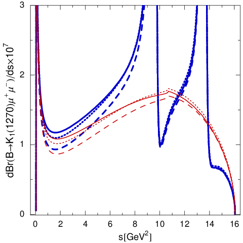
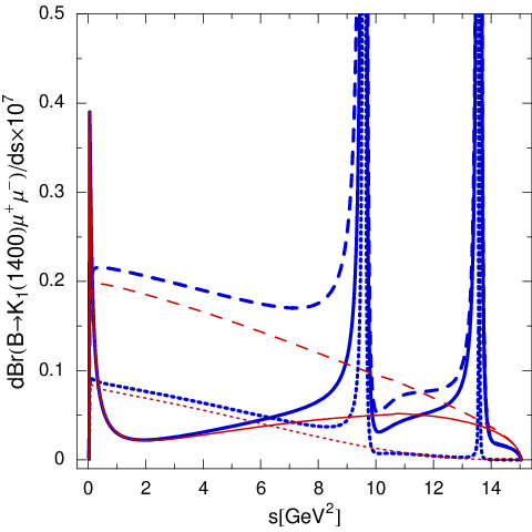
Figure 1: The dilepton invariant mass distributions for differential decay rates d​ℬ​(B−→K1−​μ+​μ−)/d​sd{\cal B}(B^{-}\to K_{1}^{-}\mu^{+}\mu^{-})/ds in the SM. The central values of inputs are used. The solid, dotted and dashed curves correspond to θK1=−34∘\theta_{K_{1}}=-34^{\circ}, −45∘-45^{\circ}, −57∘-57^{\circ}, respectively. The thick (blue) [thin (red)] curves correspond to values with [without] resonant corrections.
Refer to caption
Refer to caption

The differential decay rates d​ℬ​(B−→K1−​μ+​μ−)/d​s≡τB−×d​Γ​(B→K1−​μ+​μ−)/d​sd{\cal B}(B^{-}\to K_{1}^{-}\mu^{+}\mu^{-})/ds\equiv\tau_{B^{-}}\times d\Gamma(B\to K_{1}^{-}\mu^{+}\mu^{-})/ds are plotted in Fig. 1. To illustrate the dependence on θK1\theta_{K_{1}}, we plot the distributions for the differential decay rates with θK1=−34∘\theta_{K_{1}}=-34^{\circ}, −45∘-45^{\circ} and −57∘-57^{\circ}, respectively. The effects of charmonium resonances become large for the large region with s≳5​GeV2s\gtrsim 5{\,\mbox{GeV}}^{2}. We find that in the low ss region, where s≈2​GeV2s\approx 2{\,\mbox{GeV}}^{2}, the differential decay rate for B→K1​(1400)​μ+​μ−B\to K_{1}(1400)\mu^{+}\mu^{-} with θK1=−57∘\theta_{K_{1}}=-57^{\circ} is enhanced by about 80% compared with that with θK1=−34∘\theta_{K_{1}}=-34^{\circ}, whereas the rates for B→K1​(1270)​μ+​μ−B\to K_{1}(1270)\mu^{+}\mu^{-} is not so sensitive to variation of θK1\theta_{K_{1}}. One should note that the distribution in the low ss region is dominated by the 1/s1/s term arising from B→K1​γB\to K_{1}\gamma; for instance, for the B→K1​(1270)​μ+​μ−B\to K_{1}(1270)\mu^{+}\mu^{-} decay, it results in the peak at s∼4​mℓ2s\sim 4m_{\ell}^{2} (or exactly at s=0s=0) and contributes about −30%-30\% at around s=2​GeV2s=2{\,\mbox{GeV}}^{2} for −57∘<θK1<−34∘-57^{\circ}<\theta_{K_{1}}<-34^{\circ}.

Furthermore, the value of θK1\theta_{K_{1}} can be well determined from the following ratio of the distributions,

Rd​Γ/d​s,μ≡d​Γ​(B−→K1−​(1400)​μ+​μ−)/d​sd​Γ​(B−→K1−​(1270)​μ+​μ−)/d​s.\displaystyle R_{d\Gamma/ds,\mu}\equiv\frac{d\Gamma(B^{-}\to K_{1}^{-}(1400)\mu^{+}\mu^{-})/ds}{d\Gamma(B^{-}\to K_{1}^{-}(1270)\mu^{+}\mu^{-})/ds}. (38)

In Fig. 2, we plot the Rd​Γ/d​s,μR_{d\Gamma/ds,\mu} as a function of ss, which is highly insensitive to the resonance contributions and form factors. When the magnitude of θK1\theta_{K_{1}} is increased, this ratio peaks at about s=1.5​GeV2s=1.5{\,\mbox{GeV}}^{2} (for θK1≳40∘\theta_{K_{1}}\gtrsim 40^{\circ}).

Figure 2: The ratio of the decay distributions, Rd​Γ/d​s,μR_{d\Gamma/ds,\mu} (see the text), as a function of the dimuon invariant mass ss. The legends are the same as in Fig. 1.
Refer to caption

IV.2 Branching fractions

Figure 3: Non-resonant branching fractions ℬnr​(B−→K1−​ℓ+​ℓ−){\cal B}_{\rm nr}(B^{-}\to K_{1}^{-}\ell^{+}\ell^{-}) as functions of θK1\theta_{K_{1}}. (a) The thick solid, thick dashed, thin solid and thin dashed curves correspond to the decays B→K1​(1270)​e+​e−B\to K_{1}(1270)e^{+}e^{-}, K1​(1400)​e+​e−K_{1}(1400)e^{+}e^{-}, K1​(1270)​μ+​μ−K_{1}(1270)\mu^{+}\mu^{-} and K1​(1400)​μ+​μ−K_{1}(1400)\mu^{+}\mu^{-}, respectively. (b) The solid and dashed curves correspond to B→K1​(1270)​τ+​τ−B\to K_{1}(1270)\tau^{+}\tau^{-}, B→K1​(1400)​τ+​τ−B\to K_{1}(1400)\tau^{+}\tau^{-}, respectively. The vertical lines indicate the allowed range of θK1\theta_{K_{1}} given in Eq. (2) [26].
Refer to caption
Refer to caption
Table 6: Predictions for the non-resonant branching fractions ℬnr​(B→K1​ℓ+​ℓ−CLOSE{\cal B}_{\rm nr}(B\to{K_{1}}\ell^{+}\ell^{-}). The first and second errors come from the uncertainty of the form factors and of the θK1\theta_{K_{1}} within the allowed region [26], respectively.
Mode ℬnr×106{\cal B}_{\rm nr}\times 10^{6} Mode ℬnr×106{\cal B}_{\rm nr}\times 10^{6}
B−→K1−​(1270)​e+​e−B^{-}\to K_{1}^{-}(1270)e^{+}e^{-} 2.7−1.2−0.3+1.5+0.0{2.7}^{+{1.5}+{0.0}}_{-{1.2}-{0.3}} B¯→0K¯(1270)10e+e−\overline{B}{}^{0}\to\overline{K}{}^{0}_{1}(1270)e^{+}e^{-} 2.5−1.1−0.3+1.4+0.0{2.5}^{+{1.4}+{0.0}}_{-{1.1}-{0.3}}
B−→K1−​(1270)​μ+​μ−B^{-}\to K_{1}^{-}(1270)\mu^{+}\mu^{-} 2.3−1.0−0.2+1.3+0.0{2.3}^{+{1.3}+{0.0}}_{-{1.0}-{0.2}} B¯→0K¯(1270)10μ+μ−\overline{B}{}^{0}\to\overline{K}{}^{0}_{1}(1270)\mu^{+}\mu^{-} 2.1−0.9−0.2+1.2+0.0{2.1}^{+{1.2}+{0.0}}_{-{0.9}-{0.2}}
B−→K1−​(1270)​τ+​τ−B^{-}\to K_{1}^{-}(1270)\tau^{+}\tau^{-} 0.08−0.03−0.01+0.04+0.00{0.08}^{+{0.04}+{0.00}}_{-{0.03}-{0.01}} B¯→0K¯(1270)10τ+τ−\overline{B}{}^{0}\to\overline{K}{}^{0}_{1}(1270)\tau^{+}\tau^{-} 0.08−0.03−0.01+0.04+0.00{0.08}^{+{0.04}+{0.00}}_{-{0.03}-{0.01}}
B−→K1−​(1400)​e+​e−B^{-}\to K_{1}^{-}(1400)e^{+}e^{-} 0.10−0.03−0.05+0.03+0.25{0.10}^{+{0.03}+{0.25}}_{-{0.03}-{0.05}} B¯→0K¯(1400)10e+e−\overline{B}{}^{0}\to\overline{K}{}^{0}_{1}(1400)e^{+}e^{-} 0.09−0.03−0.04+0.03+0.23{0.09}^{+{0.03}+{0.23}}_{-{0.03}-{0.04}}
B−→K1−​(1400)​μ+​μ−B^{-}\to K_{1}^{-}(1400)\mu^{+}\mu^{-} 0.06−0.01−0.02+0.02+0.18{0.06}^{+{0.02}+{0.18}}_{-{0.01}-{0.02}} B¯→0K¯(1400)10μ+μ−\overline{B}{}^{0}\to\overline{K}{}^{0}_{1}(1400)\mu^{+}\mu^{-} 0.06−0.01−0.02+0.02+0.18{0.06}^{+{0.02}+{0.18}}_{-{0.01}-{0.02}}
B−→K1−​(1400)​τ+​τ−B^{-}\to K_{1}^{-}(1400)\tau^{+}\tau^{-} 0.001−0.000−0.001+0.000+0.005{0.001}^{+{0.000}+{0.005}}_{-{0.000}-{0.001}} B¯→0K¯(1400)10τ+τ−\overline{B}{}^{0}\to\overline{K}{}^{0}_{1}(1400)\tau^{+}\tau^{-} 0.001−0.000−0.001+0.000+0.005{0.001}^{+{0.000}+{0.005}}_{-{0.000}-{0.001}}

In Table 6, we summarize the predictions for branching fractions corresponding to θK1=−(34±13)∘\theta_{K_{1}}=-(34\pm 13)^{\circ}. The branching fractions for B→K1​e+​e−B\to{K_{1}}e^{+}e^{-} and B→K1​μ+​μ−B\to{K_{1}}\mu^{+}\mu^{-} are close to B→K∗​(892)​e+​e−B\to K^{*}(892)e^{+}e^{-}, B→K∗​(892)​μ+​μ−B\to K^{*}(892)\mu^{+}\mu^{-} given in [15]. On the other hand, the branching fractions for B→K1​τ+​τ−B\to{K_{1}}\tau^{+}\tau^{-} decays are very small since the allowed phase space is quite narrow. In Fig. 3, we plot the non-resonant branching fractions ℬnr​(B−→K1−​ℓ+​ℓ−){\cal B}_{\rm nr}(B^{-}\to K_{1}^{-}\ell^{+}\ell^{-}) as functions of θK1\theta_{K_{1}}. For the range of θK1=−(34±13)∘\theta_{K_{1}}=-(34\pm 13)^{\circ}, we obtain ℬnr​(B→K1​(1270)​ℓ+​ℓ−)≫ℬnr​(B→K1​(1400)​ℓ+​ℓ−){\cal B}_{\rm nr}(B\to K_{1}(1270)\ell^{+}\ell^{-})\gg{\cal B}_{\rm nr}(B\to K_{1}(1400)\ell^{+}\ell^{-}). It should be helpful to define the ratio,

Rℓ,nr≡ℬnr​(B→K1​(1400)​ℓ+​ℓ−)ℬnr​(B→K1​(1270)​ℓ+​ℓ−).\displaystyle R_{\ell,\rm nr}\equiv\frac{{\cal B}_{\rm nr}(B\to K_{1}(1400)\ell^{+}\ell^{-})}{{\cal B}_{\rm nr}(B\to K_{1}(1270)\ell^{+}\ell^{-})}. (39)

We show Rℓ,nrR_{\ell,\rm nr} as functions of the θK1\theta_{K_{1}} in Fig. 4. These ratios sensitively depend on θK1\theta_{K_{1}}, and are smaller than 0.150.15 for −47∘≤θK1≤−21∘-47^{\circ}\leq\theta_{K_{1}}\leq-21^{\circ}. We predict

Re,nr=0.04−0.01−0.02+0.01+0.11,Rμ,nr=0.03−0.01−0.01+0.01+0.09,Rτ,nr=0.02−0.00−0.02+0.01+0.07,\displaystyle R_{e,\rm nr}={0.04}^{+{0.01}+{0.11}}_{-{0.01}-{0.02}},\quad R_{\mu,\rm nr}={0.03}^{+{0.01}+{0.09}}_{-{0.01}-{0.01}},\quad R_{\tau,\rm nr}={0.02}^{+{0.01}+{0.07}}_{-{0.00}-{0.02}}, (40)

where the first and second errors correspond to the uncertainties of the form factors and θK1\theta_{K_{1}}, respectively. In Fig. 6, we will further show that the ratio Rμ,nrR_{\mu,\rm nr} is highly insensitive to the NP corrections.

Figure 4: Rℓ,nr≡ℬnr​(B→K1​(1400)​ℓ+​ℓ−)/ℬnr​(B→K1​(1270)​ℓ+​ℓ−)R_{\ell,\rm nr}\equiv{\cal B}_{\rm nr}(B\to K_{1}(1400)\ell^{+}\ell^{-})/{\cal B}_{\rm nr}(B\to K_{1}(1270)\ell^{+}\ell^{-}) as functions of θK1\theta_{K_{1}}. The solid, dashed and dot-dashed curves correspond to Re,nrR_{e,\rm nr}, Rμ,nrR_{\mu,\rm nr} and Rτ,nrR_{\tau,\rm nr}, respectively. The allowed range of θK1\theta_{K_{1}} given in Eq. (2) [26] is also shown.
Refer to caption

IV.3 Forward-backward asymmetry

The differential forward-backward asymmetry of the B¯→K¯1​ℓ+​ℓ−\overline{B}\to{\overline{K}_{1}}\ell^{+}\ell^{-} decay is defined by

d​AFBd​s^≡∫0u^​(s^)d​u^​d2​Γd​u^​d​s^−∫−u^​(s^)0d​u^​d2​Γd​u^​d​s^,\displaystyle\frac{dA_{\rm FB}}{d\hat{s}}\equiv\int_{0}^{\hat{u}(\hat{s})}\!d\hat{u}\frac{d^{2}\Gamma}{d\hat{u}d\hat{s}}-\int_{-\hat{u}(\hat{s})}^{0}\!d\hat{u}\frac{d^{2}\Gamma}{d\hat{u}d\hat{s}}, (41)

which can be written in terms of quantities in Eqs. (29)-(36) as

d​AFBd​s^\displaystyle\frac{dA_{\rm FB}}{d\hat{s}} =\displaystyle= −GF2​αem2​mB5210​π5|Vt​sVt​b∗|s^u^(s^)2{Re(ℬK1ℰK1∗)+Re(𝒜K1ℱK1∗)},\displaystyle-\frac{G_{F}^{2}\alpha_{\rm em}^{2}m_{B}^{5}}{2^{10}\pi^{5}}|V_{ts}V_{tb}^{*}|\hat{s}\hat{u}(\hat{s})^{2}\left\{\mathop{\mbox{Re}}\left({\cal B}^{K_{1}}{\cal E}^{{K_{1}}*}\right)+\mathop{\mbox{Re}}\left({\cal A}^{K_{1}}{\cal F}^{{K_{1}}*}\right)\right\}, (42)

and, after including the hard spectator correction [16], are given by

d​AFBd​s^\displaystyle\frac{dA_{\rm FB}}{d\hat{s}} =\displaystyle= −GF2​αem2​mB528​π5|Vt​s∗Vt​b|2s^u^(s^)2×c10[Re(c9eff(s^))AK1V1K1\displaystyle-\frac{G_{F}^{2}\alpha_{\rm em}^{2}m_{B}^{5}}{2^{8}\pi^{5}}|V_{ts}^{*}V_{tb}|^{2}\hat{s}\hat{u}(\hat{s})^{2}\times c_{10}\Bigg[\mathop{\mbox{Re}}(c_{9}^{\rm eff}(\hat{s}))A^{K_{1}}V_{1}^{K_{1}} (43)
+m^bs^c7eff{AK1T2K1(1−m^K1)+V1K1T1K1(1+m^K1)}+m^bs^ΔHS],\displaystyle\phantom{MM}+\frac{\hat{m}_{b}}{\hat{s}}c_{7}^{\rm eff}\bigg\{A^{K_{1}}T_{2}^{K_{1}}(1-\hat{m}_{K_{1}})+V_{1}^{K_{1}}T_{1}^{K_{1}}(1+\hat{m}_{K_{1}})\bigg\}+\frac{\hat{m}_{b}}{\hat{s}}\Delta_{\rm HS}\Bigg],

where ΔHS\Delta_{\rm HS} is the hard spectator correction given by

ΔHS\displaystyle\Delta_{\rm HS} =\displaystyle= {(1+m^K1)​V1K1+(1−m^K1)​(1−s^)​AK1}\displaystyle\bigg\{(1+\hat{m}_{{K_{1}}})V_{1}^{{K_{1}}}+(1-\hat{m}_{{K_{1}}})(1-\hat{s})A^{{K_{1}}}\bigg\} (44)
×αs​(μh)​CF4​π​π2Nc​fB​fK1⟂λB,+​mB​∫01d​u​ΦK1⟂​(u)​T⟂,+(nf)​(u),.\displaystyle\phantom{M}\times\frac{\alpha_{s}(\mu_{h})C_{F}}{4\pi}\frac{\pi^{2}}{N_{c}}\frac{f_{B}f_{{K_{1}}}^{\perp}}{\lambda_{B,+}m_{B}}\int_{0}^{1}\!\!\!du\,\Phi_{{K_{1}}}^{\perp}(u)T^{(\rm nf)}_{\perp,+}(u),.

Here fK1⟂f_{{K_{1}}}^{\perp} and ΦK1⟂​(u)\Phi_{{K_{1}}}^{\perp}(u) are the transverse decay constant and the twist-2 tensor light-cone distribution amplitude of the K1{K_{1}}, respectively. fK1​(1270)⟂f_{K_{1}(1270)}^{\perp}, fK1​(1400)⟂f_{K_{1}(1400)}^{\perp} and ΦK1​(1270)⟂\Phi_{K_{1}(1270)}^{\perp}, ΦK1​(1400)⟂\Phi_{K_{1}(1400)}^{\perp} are related with fK1​A⟂f_{K_{1A}}^{\perp}, fK1​B⟂f_{K_{1B}}^{\perp} and ΦK1​A⟂\Phi_{K_{1A}}^{\perp}, ΦK1​B⟂\Phi_{K_{1B}}^{\perp} by [35]

(fK1​(1270)⟂fK1​(1400)⟂)\displaystyle\pmatrix{f_{K_{1}(1270)}^{\perp}\cr f_{K_{1}(1400)}^{\perp}} =\displaystyle= M⋅(fK1​A⟂​a0K1​A,⟂fK1​B⟂),\displaystyle M\cdot\pmatrix{f_{K_{1A}}^{\perp}a_{0}^{K_{1A},\perp}\cr f_{K_{1B}}^{\perp}}, (45)
(fK1​(1270)⟂​ΦK1​(1270)⟂fK1​(1400)⟂​ΦK1​(1400)⟂)\displaystyle\pmatrix{f_{K_{1}(1270)}^{\perp}\Phi_{K_{1}(1270)}^{\perp}\cr f_{K_{1}(1400)}^{\perp}\Phi_{K_{1}(1400)}^{\perp}} =\displaystyle= M⋅(fK1​A⟂​ΦK1​A⟂fK1​B⟂​ΦK1​B⟂),\displaystyle M\cdot\pmatrix{f_{K_{1A}}^{\perp}\Phi_{K_{1A}}^{\perp}\cr f_{K_{1B}}^{\perp}\Phi_{K_{1B}}^{\perp}}, (46)

where ΦK1​A⟂\Phi_{K_{1A}}^{\perp} and ΦK1​B⟂\Phi_{K_{1B}}^{\perp} are expanded as

ΦK1​A⟂​(u)\displaystyle\Phi_{K_{1A}}^{\perp}(u) =\displaystyle= 6​u​u¯​[a0K1​A,⟂+3​a1K1​B,⟂​ξ+a2K1​B,⟂​32​(5​ξ2−1)],\displaystyle 6u\bar{u}\left[a_{0}^{K_{1A},\perp}+3a_{1}^{K_{1B},\perp}\xi+a_{2}^{K_{1B},\perp}\frac{3}{2}(5\xi^{2}-1)\right], (47)
ΦK1​B⟂​(u)\displaystyle\Phi_{K_{1B}}^{\perp}(u) =\displaystyle= 6​u​u¯​[1+3​a1K1​B,⟂​ξ+a2K1​B,⟂​32​(5​ξ2−1)],\displaystyle 6u\bar{u}\left[1+3a_{1}^{K_{1B},\perp}\xi+a_{2}^{K_{1B},\perp}\frac{3}{2}(5\xi^{2}-1)\right], (48)

with a0K1​B,⟂≡1a_{0}^{K_{1B},\perp}\equiv 1, u¯≡1−u\bar{u}\equiv 1-u and ξ≡u−u¯\xi\equiv u-\bar{u}. The values of fK1​A⟂f_{K_{1A}}^{\perp}, fK1​B⟂f_{K_{1B}}^{\perp} and the Gegenbauer moments, aiK1,⟂a_{i}^{{K_{1}},\perp}, are tabulated in Table 5.

In the following, to compare the theoretical predictions with the data, we use the normalized differential forward-backward asymmetry as

d​A¯FBd​s^≡d​AFBd​s^/d​Γd​s^.\displaystyle\frac{\displaystyle{d\overline{A}_{\rm FB}}}{\displaystyle{d\hat{s}}}\equiv\frac{dA_{\rm FB}}{d\hat{s}}\Bigg/\frac{d\Gamma}{d\hat{s}}. (49)

In Fig. 5, the normalized differential forward-backward asymmetries d​A¯FB​(B−→K1−​μ+​μ−)/d​sd\overline{A}_{\rm FB}(B^{-}\to K_{1}^{-}\mu^{+}\mu^{-})/ds versus ss are plotted. For B→K1​(1270)​μ+​μ−B\to K_{1}(1270)\mu^{+}\mu^{-} decays, the dependence of d​A¯FB/d​sd\overline{A}_{\rm FB}/ds on θK1\theta_{K_{1}} is negligibly small. For θK1≲−45∘\theta_{K_{1}}\lesssim-45^{\circ}, d​A¯FB​(B→K1​(1400)​μ+​μ−)/d​sd\overline{A}_{\rm FB}(B\to K_{1}(1400)\mu^{+}\mu^{-})/ds almost vanishes in the region below the J/ψJ/\psi resonance. We define s0K1s_{0}^{K_{1}} to be the position of zero of the FBA. s0K1s_{0}^{K_{1}} satisfies

Re⁡(c9eff​(s^0K1))c7eff,HS​(s^0K1)\displaystyle\frac{\mathop{\mbox{Re}}(c_{9}^{\rm eff}(\hat{s}_{0}^{K_{1}}))}{c_{7}^{{\rm eff},{\rm HS}}(\hat{s}_{0}^{{K_{1}}})} =\displaystyle= −m^bs^0K1​{T2K1​(s^0K1)V1K1​(s^0K1)​(1−m^K1)+T1K1​(s^0K1)AK1​(s^0K1)​(1+m^K1)},\displaystyle-\frac{\hat{m}_{b}}{\hat{s}_{0}^{K_{1}}}\left\{\frac{T_{2}^{K_{1}}(\hat{s}_{0}^{K_{1}})}{V_{1}^{K_{1}}(\hat{s}_{0}^{K_{1}})}(1-\hat{m}_{K_{1}})+\frac{T_{1}^{K_{1}}(\hat{s}_{0}^{K_{1}})}{A^{K_{1}}(\hat{s}_{0}^{K_{1}})}(1+\hat{m}_{K_{1}})\right\}, (50)

which is negative. Here

c7eff,HS​(s^)\displaystyle c_{7}^{{\rm eff},{\rm HS}}(\hat{s}) ≡\displaystyle\equiv c7eff+ΔHS​(s^)AK1​(s^)​T2K1​(s^)​(1−m^K1)+V1K1​(s^)​T1K1​(s^)​(1+m^K1).\displaystyle c_{7}^{{\rm eff}}+\frac{\Delta_{\rm HS}(\hat{s})}{A^{{K_{1}}}(\hat{s})T_{2}^{{K_{1}}}(\hat{s})(1-\hat{m}_{{K_{1}}})+V_{1}^{{K_{1}}}(\hat{s})T_{1}^{{K_{1}}}(\hat{s})(1+\hat{m}_{K_{1}})}. (51)

The position of zero appears below the J/ψJ/\psi-resonance region and depends weakly on θK1\theta_{K_{1}}, especially for B→K1​(1270)​ℓ+​ℓ−B\to K_{1}(1270)\ell^{+}\ell^{-} as shown in Fig. 5. We obtain the positions of the zeros of forward-backward asymmetries to be

s0K1​(1270)=2.27−0.07−0.01+0.04+0.01​GeV2 and s0K1​(1400)=2.80−0.29−0.07+0.23+0.74​GeV2,\displaystyle s_{0}^{K_{1}(1270)}={2.27}^{+{0.04}+{0.01}}_{-{0.07}-{0.01}}{\,\mbox{GeV}}^{2}\quad\mbox{ and }\quad s_{0}^{K_{1}(1400)}={2.80}^{+{0.23}+{0.74}}_{-{0.29}-{0.07}}{\,\mbox{GeV}}^{2}, (52)

where the first and second errors correspond to the uncertainties of the form factors and θK1(=−(34±13)∘)\theta_{K_{1}}(=-(34\pm 13)^{\circ}), respectively. In the following section, we will show that, as the B→K∗​(892)​ℓ+​ℓ−B\to K^{*}(892)\ell^{+}\ell^{-} decay, for the B→K1​(1270)​ℓ+​ℓ−B\to K_{1}(1270)\ell^{+}\ell^{-} decay the position of the zero of the FBA can be a good observable for searching for new-physics effects.
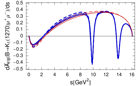
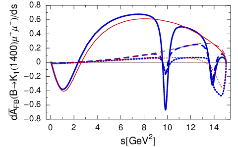
Figure 5: Normalized differential forward-backward asymmetries: (a) d​A¯FB​(B−→K1−​(1270)​μ+​μ−)/d​sd\overline{A}_{\rm FB}(B^{-}\to K_{1}^{-}(1270)\mu^{+}\mu^{-})/ds and (b) d​A¯FB​(B−→K1−​(1400)​μ+​μ−)/d​sd\overline{A}_{\rm FB}(B^{-}\to K_{1}^{-}(1400)\mu^{+}\mu^{-})/ds. The legends are the same as Fig. 1.
Refer to caption
Refer to caption

V NP effects

In this section, we study the NP corrections to the B−→K1−​μ+​μ−B^{-}\to K_{1}^{-}\mu^{+}\mu^{-} decays in the model-independent way. As in Ref. [15], we parametrize the NP contributions to the Wilson coefficients as

ci≡ciSM+ciNP=Ri​ciSM for ci=c7eff,c9,c10,\displaystyle c_{i}\equiv c_{i}^{{\rm SM}}+c_{i}^{{\rm NP}}=R_{i}\,c_{i}^{{\rm SM}}\quad\mbox{ for }\quad c_{i}=c_{7}^{{\rm eff}},c_{9},c_{10}, (53)

at the scale m¯b​(m¯b)\overline{m}_{b}(\overline{m}_{b}). For simplicity, we assume all RiR_{i} are real. The model-independent analysis for B→Xs​γB\to X_{s}\gamma and B→Xs​ℓ+​ℓ−B\to X_{s}\ell^{+}\ell^{-} [17] gives the following constraints,

0.8≲|R7|≲1.2,1≲R92+R102≲4.\displaystyle 0.8\lesssim|R_{7}|\lesssim 1.2,\quad 1\lesssim R_{9}^{2}+R_{10}^{2}\lesssim 4. (54)

The possibility of flipped sign of c7effc_{7}^{\rm eff} due to the NP contribution in the minimum supersymmetric standard model (MSSM) with the minimal flavor violation (MFV) ansatz and with large tan⁡β\tan\beta has been studied in Ref. [18]. The twofold constraint was given by

−0.02≤c7NP≤0.12or0.59≤c7NP≤1.24,\displaystyle-0.02\leq c_{7}^{{\rm NP}}\leq 0.12\quad\mbox{or}\quad 0.59\leq c_{7}^{{\rm NP}}\leq 1.24, (55)

at the weak scale. Further constraints on c7NPc_{7}^{{\rm NP}} have been obtained with

c7NP\displaystyle c_{7}^{{\rm NP}} =\displaystyle= −0.039±0.043∪0.931±0.016(68% CL)\displaystyle-0.039\pm 0.043\cup 0.931\pm 0.016\quad\mbox{($68\%$ CL)} (56)
=\displaystyle= [−0.104,0.026]∪[0.874,0.988](95% CL)\displaystyle[-0.104,0.026]\cup[0.874,0.988]\quad\mbox{($95\%$ CL)} (57)

in Ref. [37] and

c7NP\displaystyle c_{7}^{{\rm NP}} =\displaystyle= 0.02±0.047∪0.958±0.002(68% CL)\displaystyle 0.02\pm 0.047\cup 0.958\pm 0.002\quad\mbox{($68\%$ CL)} (58)
=\displaystyle= [−0.039,0.08]∪[0.859,1.031](95% CL)\displaystyle[-0.039,0.08]\cup[0.859,1.031]\quad\quad\mbox{($95\%$ CL)} (59)

in Ref. [38]. The sign of Re(c7effc_{7}^{\rm eff}) can also be flipped in supersymmetric models with non-minimal flavor violation via gluino-down-squark loops. Furthermore, in general flavor-violating supersymmetric models the sign of c9c_{9} and c10c_{10} can be flipped. Therefore, in the present paper, we consider Ri=1.2R_{i}=1.2 (i.e. 20%20\% enhancement for the SM Wilson coefficients due to the NP correction), 1.01.0 (i.e. without the NP correction), 0.80.8 (i.e. 20%20\% smaller than the SM Wilson coefficients) and −1.0-1.0 (i.e. the Wilson coefficients are in opposite signs but have the same magnitudes compared to the SM results).

In Fig. 6, the ratio of the non-resonant branching fractions Rμ,nr≡ℬnr​(B→K1​(1400)​μ+​μ−)/ℬnr​(B→K1​(1270)​μ+​μ−)R_{\mu,\rm nr}\equiv{\cal B}_{\rm nr}(B\to K_{1}(1400)\mu^{+}\mu^{-})/{\cal B}_{\rm nr}(B\to K_{1}(1270)\mu^{+}\mu^{-}), including the NP corrections, as a function of the value of θK1\theta_{K_{1}} is depicted. We show that Rμ,nrR_{\mu,\rm nr} is highly insensitive to the NP effect and thus is suitable for determining the value of θK1\theta_{K_{1}}. In Fig. 7, we plot Rd​Γ/d​s,μR_{d\Gamma/ds,\mu}, the ratio of the differential decay rates, as a function of the dimuon invariant mass, ss, where the NP effects are considered. We find that Rd​Γ/d​s,μR_{d\Gamma/ds,\mu} is insensitive to variation of R10R_{10}, whereas its value is increased (decreased) by about 100%100\% (40%40\%) at about s=1.5​GeV2s=1.5{\,\mbox{GeV}}^{2} corresponding to θK1=−34∘\theta_{K_{1}}=-34^{\circ} (−57∘-57^{\circ}) when R7R_{7} or R9R_{9} equals to −1-1.

Figure 6: Rμ,nr=ℬnr​(B→K1​(1400)​μ+​μ−)/ℬnr​(B→K1​(1270)​μ+​μ−)R_{\mu,\rm nr}={\cal B}_{\rm nr}(B\to K_{1}(1400)\mu^{+}\mu^{-})/{\cal B}_{\rm nr}(B\to K_{1}(1270)\mu^{+}\mu^{-}) as a function of θK1\theta_{K_{1}}. Variations of NP with (R7,R9,R10)=(r,1,1),(1,r,1),(R_{7},R_{9},R_{10})=(r,1,1),(1,r,1), and (1,1,r)(1,1,r) are respectively included, where r=1.0r=1.0 (solid), 1.21.2 (dotted), 0.80.8 (dot-dashed) and −1.0-1.0 (dashed). The vertical lines indicate the allowed range of θK1\theta_{K_{1}} given in Eq. (2) [26].
Refer to caption
Figure 7: Rd​Γ/d​s,μR_{d\Gamma/ds,\mu}, the ratio of the differential decay rates, as a function of the dimuon invariant mass, ss. Variations of R7R_{7}, R9R_{9} and R10R_{10} are depicted in (a), (b) and (c) respectively, where the remaining RiR_{i} are set to their SM values. The thick (blue) and thin (red) curves correspond to θK1=−34∘\theta_{K_{1}}=-34^{\circ} and −57∘-57^{\circ}, respectively. The solid, dotted, dot-dashed and dashed curves correspond to Ri=1.0R_{i}=1.0, 1.21.2, 0.80.8 and −1.0-1.0, respectively.
Refer to caption
Refer to caption
Refer to caption

Taking into account the possible NP corrections, we plot d​A¯FB​(B−→K1−​(1270)​μ+​μ−)/d​sd\overline{A}_{\rm FB}(B^{-}\to K_{1}^{-}(1270)\mu^{+}\mu^{-})/ds as a function of ss in Fig. 8. We do not consider the B−→K1−​(1400)​μ+​μ−B^{-}\to K_{1}^{-}(1400)\mu^{+}\mu^{-} decay, since its branching fraction is relatively small. As shown in Fig. 5 (see also Fig. 8), the differential forward-backward asymmetry for B→K1​(1270)​μ+​μ−B\to K_{1}(1270)\mu^{+}\mu^{-} and its s0K1​(1270)s_{0}^{K_{1}(1270)} (if existing) are very insensitive to variation of θK1\theta_{K_{1}}. For the cases with c7eff,c9c_{7}^{\rm eff},c_{9} and c10c_{10} of SM-like sign, the change of the FBA zero owing to variation of NP parameters could be manifest as compared to the hadronic uncertainties. As is well known in the case of B→K∗​(892)​ℓ+​ℓ−B\to K^{*}(892)\ell^{+}\ell^{-}, for the flipped sign of c7eff,c9c_{7}^{\rm eff},c_{9} or c10c_{10} the characteristic features of the FBA change dramatically. Because the asymmetry zero exists only for Re⁡(c9eff)/c7eff<0\mathop{\mbox{Re}}(c_{9}^{\rm eff})/c_{7}^{\rm eff}<0 (see Eq. (50)), therefore there is no asymmetry zero for (R7,R9)=(±1,∓1)(R_{7},R_{9})=(\pm 1,\mp 1) in the spectrum. Flipping the sign of c10c_{10} would change the sign of the FBA. From the above discussions we can conclude that the position of the FBA zero for the B→K1​(1270)​ℓ+​ℓ−B\to K_{1}(1270)\ell^{+}\ell^{-} decay is a suitable quantity to constrain the NP parameters. Recent measurements for B→K∗​(892)​ℓ+​ℓ−B\to K^{*}(892)\ell^{+}\ell^{-} decays [8, 9] seem to favor (i) the flipped sign of c7effc_{7}^{{\rm eff}} which is denoted by the dashed curves in Fig. 8(a), or (ii) the simultaneous flip of the sign of c9c_{9} and c10c_{10} which are denoted by the double-dot dashed curves in Fig. 8(c). However, they disfavor the flipped sign(c9​c10c_{9}c_{10}) models. See also the discussion in Ref. [20].

Figure 8: Normalized differential forward-backward asymmetry d​A¯FB​(B−→K1−​(1270)​μ+​μ−)/d​sd\overline{A}_{\rm FB}(B^{-}\to K_{1}^{-}(1270)\mu^{+}\mu^{-})/ds as a function of the dimuon invariant mass ss. The thick (blue) and thin (red) curves correspond to the asymmetries with θK1=−34∘\theta_{K_{1}}=-34^{\circ} and −57∘-57^{\circ}, respectively. In (a), where R9=R10=1.0R_{9}=R_{10}=1.0 (the SM result), the solid curves are for R7=1.0R_{7}=1.0, the dotted for R7=1.2R_{7}=1.2, the dot-dashed for R7=0.8R_{7}=0.8 and the dashed for R7=−1.0R_{7}=-1.0. In (b), where R7=R10=1.0R_{7}=R_{10}=1.0 (the SM result), and the solid curves are for R9=1.0R_{9}=1.0, the dotted for R9=1.2R_{9}=1.2, the dot-dashed for R9=0.8R_{9}=0.8 and the dashed for R9=−1.0R_{9}=-1.0. In (c), where R7=R9=1.0R_{7}=R_{9}=1.0 and the solid curves are for R10=1.0R_{10}=1.0 (the SM result), the dotted for R10=1.2R_{10}=1.2, the dot-dashed for R10=0.8R_{10}=0.8 and the dashed for R10=−1.0R_{10}=-1.0. The d​A¯FB/d​sd\overline{A}_{\rm FB}/ds with (R7,R9,R10)=(1.0,−1.0,−1.0)(R_{7},R_{9},R_{10})=(1.0,-1.0,-1.0), and (−1.0,1.0,−1.0)(-1.0,1.0,-1.0) are denoted by the double-dot dashed and long-short dashed curves, respectively, in (c).
Refer to caption
Refer to caption
Refer to caption

VI Summary

We have studied the rare decays B→K1​ℓ+​ℓ−B\to K_{1}\ell^{+}\ell^{-} with K1≡K1​(1270)K_{1}\equiv K_{1}(1270), K1​(1400)K_{1}(1400) and ℓ≡e\ell\equiv e, μ\mu, τ\tau. The strange axial-vector mesons, K1​(1270)K_{1}(1270) and K1​(1400)K_{1}(1400), are the mixtures of the K1​AK_{1A} and K1​BK_{1B}, which are the 13​P11^{3}P_{1} and 11​P11^{1}P_{1} states, respectively. Although the branching ratios depend on the magnitudes of B→K1B\to K_{1} form factors, the K1​(1270)K_{1}(1270)–K1​(1400)K_{1}(1400) mixing angle, θK1\theta_{K_{1}}, can be well determined from the measurement of the ratio Rℓ≡ℬ⁡(B→K1​(1400)​ℓ+​ℓ−)/ℬ⁡(B→K1​(1270)​ℓ+​ℓ−)R_{\ell}\equiv{\cal B}(B\to K_{1}(1400)\ell^{+}\ell^{-})/{\cal B}(B\to K_{1}(1270)\ell^{+}\ell^{-}), which depends very weakly on new-physics corrections. We have calculated differential forward-backward asymmetries of B→K1​μ+​μ−B\to K_{1}\mu^{+}\mu^{-} decays. For B→K1​(1270)​μ+​μ−B\to K_{1}(1270)\mu^{+}\mu^{-}, the asymmetry zero, which depends very weakly on θK1\theta_{K_{1}}, can be dramatically changed due to variation of new-physics parameters.

Acknowledgements.
This research was supported in part by the National Science Council of R.O.C. under Grant No. NSC96-2112-M-033-004-MY3 and No. NSC96-2811-M-033-004.

References

  • [1] E. Barberio et al., arXiv:0808.1297 [hep-ex].
  • [2] B. Aubert et al. [BABAR Collaboration], Phys. Rev. D 70, 112006 (2004) [arXiv:hep-ex/0407003].
  • [3] M. Nakao et al. [Belle Collaboration], Phys. Rev. D 69, 112001 (2004) [arXiv:hep-ex/0402042].
  • [4] T. E. Coan et al. [CLEO Collaboration], Phys. Rev. Lett. 84, 5283 (2000) [arXiv:hep-ex/9912057].
  • [5] H. Yang et al., Phys. Rev. Lett. 94, 111802 (2005) [arXiv:hep-ex/0412039].
  • [6] A. Ishikawa et al. [Belle Collaboration], Phys. Rev. Lett. 91, 261601 (2003) [arXiv:hep-ex/0308044].
  • [7] B. Aubert et al. [BABAR Collaboration], Phys. Rev. D 73, 092001 (2006) [arXiv:hep-ex/0604007].
  • [8] A. Ishikawa et al. [Belle Collaboration], Phys. Rev. Lett. 96, 251801 (2006) [arXiv:hep-ex/0603018].
  • [9] B. Aubert et al. [BABAR Collaboration], arXiv:0804.4412 [hep-ex].
  • [10] B. Aubert et al. [BABAR Collaboration], arXiv:0807.4119 [hep-ex].
  • [11] G. Eigen, arXiv:0807.4076 [hep-ex].
  • [12] M. A. Paracha, I. Ahmed and M. J. Aslam, Eur. Phys. J. C 52, 967 (2007) [arXiv:0707.0733 [hep-ph]].
  • [13] I. Ahmed, M. A. Paracha and M. J. Aslam, Eur. Phys. J. C 54, 591 (2008) [arXiv:0802.0740 [hep-ph]].
  • [14] A. Saddique, M. J. Aslam and C. D. Lu, arXiv:0803.0192 [hep-ph].
  • [15] A. Ali, P. Ball, L. T. Handoko and G. Hiller, Phys. Rev. D 61, 074024 (2000) [arXiv:hep-ph/9910221].
  • [16] M. Beneke, T. Feldmann and D. Seidel, Nucl. Phys. B 612, 25 (2001) [arXiv:hep-ph/0106067].
  • [17] A. Ali, E. Lunghi, C. Greub and G. Hiller, Phys. Rev. D 66, 034002 (2002) [arXiv:hep-ph/0112300].
  • [18] T. Feldmann and J. Matias, JHEP 0301, 074 (2003) [arXiv:hep-ph/0212158].
  • [19] F. Kruger and J. Matias, Phys. Rev. D 71, 094009 (2005) [arXiv:hep-ph/0502060].
  • [20] C. Bobeth, G. Hiller and G. Piranishvili, JHEP 0807, 106 (2008) [arXiv:0805.2525 [hep-ph]].
  • [21] U. Egede, T. Hurth, J. Matias, M. Ramon and W. Reece, arXiv:0807.2589 [hep-ph].
  • [22] C. H. Chen, C. Q. Geng and L. Li, arXiv:0808.0127 [hep-ph].
  • [23] M. Suzuki, Phys. Rev. D 47, 1252 (1993).
  • [24] L. Burakovsky and J. T. Goldman, Phys. Rev. D 57, 2879 (1998) [arXiv:hep-ph/9703271].
  • [25] H. Y. Cheng, Phys. Rev. D 67, 094007 (2003) [arXiv:hep-ph/0301198].
  • [26] H. Hatanaka and K. C. Yang, Phys. Rev. D 77, 094023 (2008) [arXiv:0804.3198 [hep-ph]].
  • [27] A. J. Buras, M. Misiak, M. Munz and S. Pokorski, Nucl. Phys. B 424, 374 (1994) [arXiv:hep-ph/9311345].
  • [28] A. J. Buras and M. Munz, Phys. Rev. D 52, 186 (1995) [arXiv:hep-ph/9501281].
  • [29] C. S. Lim, T. Morozumi and A. I. Sanda, Phys. Lett. B 218, 343 (1989).
  • [30] A. Ali, T. Mannel and T. Morozumi, Phys. Lett. B 273, 505 (1991).
  • [31] F. Kruger and L. M. Sehgal, Phys. Lett. B 380, 199 (1996) [arXiv:hep-ph/9603237].
  • [32] W. M. Yao et al. [Particle Data Group], J. Phys. G 33, 1 (2006).
  • [33] K. C. Yang, Phys. Rev. D 78, 034018 (2008) [arXiv:0807.1171 [hep-ph]].
  • [34] K. C. Yang, in preparation.
  • [35] K. C. Yang, Nucl. Phys. B 776, 187 (2007) [arXiv:0705.0692 [hep-ph]].
  • [36] CKM fitter group (URL: http://ckmfitter.in2p3.fr).
  • [37] U. Haisch and A. Weiler, Phys. Rev. D 76, 074027 (2007) [arXiv:0706.2054 [hep-ph]].
  • [38] C. Bobeth, M. Bona, A. J. Buras, T. Ewerth, M. Pierini, L. Silvestrini and A. Weiler, Nucl. Phys. B 726, 252 (2005) [arXiv:hep-ph/0505110].