Hyperon Polarization in Unpolarized Scattering Processes

Single transverse spin asymmetry (SSA) phenomena have a long history, starting with the observation of large transverse polarization of Hyperon ($\Lambda$) in unpolarized nucleon-nucleon scattering [1, 2]. It has imposed theoretical challenges to understand these phenomena in Quantum Chromodynamics (QCD) [2, 3]. In recent years, this physics has attracted strong interests from both experiment and theory sides. For example, the experimental observation of SSAs in semi-inclusive hadron production in deep inelastic scattering (SIDIS), in inclusive hadron production in $pp$ scattering at collider energy at RHIC, and the relevant azimuthal asymmetric distribution of hadron production in $e^{+}e^{-}$ annihilation have motivated theoretical developments in the last few years  [4, 5, 6, 7, 8, 9]. Among these developments, two mechanisms in the QCD framework have been most explored to study the large SSAs observed in the experiments. One is the so-called twist-three quark-gluon correlation approach  [3, 10, 11, 12, 14, 13, 15], and the other is the transverse momentum dependent (TMD) approach where the intrinsic transverse momentum of partons inside nucleon plays important role  [4, 5, 6, 7, 16, 17]. Recent studies have shown that these two approaches are consistent to each other in the intermediate transverse momentum region where both apply [18].

In particular, theoretical developments have been made to understand the $\Lambda$ polarization in unpolarized hadronic reactions [19, 20, 22, 21]. Similar to the SSA in inclusive hadron production in $p^{\uparrow}p\to\pi X$, the Hyperon polarization in unpolarized $pp$ scattering $pp\to\Lambda_{\uparrow}X$ receives the contributions from (naive)-time-reversal-odd effects in the distribution and fragmentation parts [22, 21]. In order to understand the experimental observations of $pp\to\Lambda_{\uparrow}X$, one has to take into account both contributions.

On the other hand, in the deep inelastic scattering process, one can separate these two contributions because they have different azimuthal angle dependence [23]. To describe these effects, one can calculate the $\Lambda$ polarization in the twist-three approach [22] or use the TMD mechanism [23]. For example, the contribution from the T-odd effects in the distribution part is associated with the so-called Boer-Mulders TMD quark distribution $h_{1}^{\perp}$ [23] multiplied by the TMD transversity fragmentation function $H_{1T}$ when the transverse momentum of the produced $\Lambda$ is much smaller than the hard scale $P_{\Lambda\perp}\ll Q$ where $Q$ is the virtuality of the virtual photon in DIS process. On the other hand, we can also calculate this contribution from the twist-three mechanism when the transverse momentum is much larger than the nonperturbative scale $\Lambda_{\rm QCD}$: $P_{\Lambda\perp}\gg\Lambda_{\rm QCD}$. From our calculations, we find that these two approaches indeed provide a unique description for $\Lambda$ polarization at the intermediate transverse momentum region in the semi-inclusive DIS. The large transverse momentum Boer-Mulders function calculated in this context can also be used in other processes, like Drell-Yan lepton pair production in $pp$ scattering [24].

The rest of the paper is organized as follows. In Sec.II, we study the $\Lambda$ polarization in semi-inclusive deep inelastic scattering $e+p\rightarrow e+\Lambda_{\uparrow}+X$ by calculating the contribution from the twist-three quark-gluon-antiquark correlation function from nucleon. We will then take the limit of small transverse momentum $P_{\Lambda\perp}\ll Q$, and compare to the prediction from the TMD factorization approach. In the TMD picture, the polarization of $\Lambda$ comes from the Beor-Mulders function $h_{1}^{\perp}$. In Sec.III, we extend our calculations to the Hyperon polarization in $pp$ collisions, and compare to the previous results. We conclude in Sec. IV.

In the SIDIS process $ep\rightarrow e^{\prime}\Lambda_{\uparrow}X$ , the differential cross section can be formulated as

where $\alpha_{em}$ is the electromagnetic coupling, $l$ and $P$ are incoming momenta for the lepton and nucleon, $q$ the momentum for the exchanged virtual photon with $Q^{2}=-q.q$, $P_{\Lambda}$ and $S_{\Lambda\perp}$ are the momentum and transverse polarization vector for the final state $\Lambda$, respectively, and we have $S_{\Lambda\perp}\cdot P_{\Lambda}=0$. The kinematic variables are defined as $x_{B}=\frac{Q^{2}}{2P\cdot q}$, $z_{h}=\frac{P\cdot P_{\Lambda}}{P\cdot q}$, $y=\frac{P\cdot q}{P\cdot l}$. In the above equation, $L^{\mu\nu}$ and $W^{\mu\nu}$ are the leptonic and hadronic tensors, respectively. They are given by,

where $l^{\prime}$ is the momentum for the final state lepton, $J^{\mu}$ is the quark electromagnetic current, and $X$ represents all other final-state hadrons other than the observed Hyperon $\Lambda$.

It is convenient to write the momentum of the virtual photon in terms of the incoming and outgoing hadron momenta,

where $q_{t}^{\mu}$ is transverse to the momentum of the initial and final hadrons: $q_{t}^{\mu}P_{\mu}=q_{t}^{\mu}P_{\Lambda\mu}=0$. Here $q_{t}^{\mu}$ is a space-like vector, and we define $\vec{q}^{\ 2}_{\perp}\equiv-q_{t}^{2}$. In the hadron frame, the final state hadron will have the momentum,

where $P_{\Lambda\perp}$ is the Hyperon transverse momentum in the hadron-frame, $P^{+}=1/\sqrt{2}(P^{0}+P^{z})$, and we use the conventional definition for light-cone vector $p^{\mu},n^{\mu}$: $p=(1^{+},0^{-},0_{\perp})$, $n=(0^{+},1^{-},0_{\perp})$. From the above definitions, we will find $\vec{q}^{\ 2}_{\perp}=\vec{P}_{\Lambda\perp}^{\ 2}/{z_{h}^{2}}$.

We will calculate the hadronic tensor $W^{\mu\nu}$ at large transverse momentum in perturbative QCD, by radiating a hard gluon in the final state. They are expressed in terms of integrated parton distribution and fragmentation functions or the quark-gluon-antiquark correlations, according to a collinear factorization [25]. In the calculations, it is convenient to decompose the hadronic tensor $W^{\mu\nu}$ in terms of individual tensors [26, 27],

where the $W_{i}$ are structure functions, and can be projected out from $W^{\mu\nu}$ by $W_{i}=W_{\alpha\beta}\tilde{V}_{i}^{\alpha\beta}$ with the corresponding inverse tensors $\tilde{V}_{i}$. Both $V_{i}$, $\tilde{V}_{i}$ can be constructed from four orthonormal basis vectors [26]: $T^{\mu},X^{\mu},Y^{\mu},Z^{\mu}$ with normalization $T^{\mu}T_{\mu}=1,X^{\mu}X_{\mu}=Y^{\mu}Y_{\mu}=Z^{\mu}Z_{\mu}=-1$. These four vectors can be further constructed by $P^{\mu}$, $q^{\mu}$, $S_{\Lambda\perp}^{\mu}$, $q_{t}^{\mu}$. In this paper, we choose a special frame, where the $q_{t}^{\mu}$ is parallel to $X^{\mu}$, and the target proton and final state $\Lambda$ have spatial components only in the $Z$ direction. In the small $q_{t}$ ($P_{\Lambda\perp}$) region, we have checked that this frame leads to the same result as that in the normal hadron frame.

As mentioned in the Introduction, in this paper, we are interested in calculating the differential cross section in the intermediate transverse momentum region, $\Lambda_{QCD}\ll P_{\Lambda\perp}\ll Q$. In the calculations, we will utilize the power counting method, and only keep the leading power contributions and neglect all higher order corrections in terms of $P_{\Lambda\perp}/Q$. For the spin-average $\Lambda$ production in SIDIS, the differential cross section will be identical to any other hadron production process except we have to change the associated fragmentation function for the Hyperon. This cross section in the above limit will be consistent to the TMD factorization approach in the intermediate transverse momentum region as what has been shown before, for example, in the pion production in SIDIS [18].

For the $\Lambda$ polarization dependent cross section, we have two separate contributions from the twist-three quark-gluon-antiquark correlations in the parton distribution or fragmentation. In this paper, we will only focus on the parton distribution part, whereas that from the fragmentation part can follow accordingly. We also note that these two contributions will have different azimuthal angular dependence in SIDIS in the small transverse momentum limit. For the contribution from the parton distribution part, following the Qiu-Sterman formalism, the corresponding spin-dependent hadronic tensor can be written as [3],

where $T$ and $H$ represent the twist-three function and the partonic hard-scattering amplitude, respectively. These two parts are connected by the two independent integrals over the momentum $k_{1}$ and $k_{2}$ that they share. In the above expansion, spinor and color indices connecting the hard part and long-distance parts have already been separated, which leads to the hard part $H(k_{1},k_{2},P_{\Lambda\perp},S_{\Lambda\perp})$ being contracted with $(1/2)\not\!\!p\gamma^{\rho}_{\perp}/(2\pi)$. The transversity fragmentation $H_{1T}$ for $\Lambda$ production is defined as

where $X$ represents all other particles in the final state except for $\Lambda$, $S_{\perp}^{\mu}$ is the transverse polarization vector of the final state hadron. The next step is to perform a collinear expansion of the expression:

where minus component has been neglected since it is beyond the order in $k_{i,\perp}$ that we consider. The collinear expansion enables us to reduce the four-dimensional integral to a integral convolution in the light-cone momentum fractions of the initial partons. Expanding $H^{\mu\nu}$ in the partonic momentum at $k_{1}=x_{1}P$ and $k_{2}=x_{2}P$, we have

The above expansion allows us to integrate over three of the four components of each of the loop momenta $k_{i}$, and the hadronic tensor $W^{\mu\nu}$ will depend on the chiral-odd spin-independent twist-three quark-gluon-antiquark correlation function [3, 22],

where the sums over color and spin indices are implicit, $|P\rangle$ denotes the unpolarized proton state, $\psi$ is the quark field, and $F_{+\mu}$ the gluon field tensor, and the gauge link has been suppressed. Due to parity and time-reversal invariance, we have the relation $T_{F}^{(\sigma)}(x_{1},x_{2})=T_{F}^{(\sigma)}(x_{2},x_{1})$.

Similar to the SSA in $\pi$ production in SIDIS, the strong interaction phase necessary for having a non-vanishing $\Lambda$ transverse polarization arises from the interference between an imaginary part of the partonic scattering amplitude with the extra gluon and the real scattering amplitude without a gluon. The imaginary part is due to the pole of the parton propagator associated with the integration over the gluon momentum fraction $x_{g}$ . Depending on which propagator’s pole contributes, the amplitude may get contributions from $x_{g}=0$ (“soft-pole”) and $x_{g}\neq 0$ (“hard-pole” or “soft-fermion-pole”) [18]. The diagrams contributing to the $\Lambda$ polarization in SIDIS will be the same as those calculated for the SSA in $\pi$ production. The only difference is that we have to replace the Qiu-Sterman matrix element $T_{F}$ with the above unpolarized quark-gluon-antiquark correlation function $T_{F}^{(\sigma)}$, and the unpolarized fragmentation function $D(z)$ for $\pi$ with the transversity fragmentation function for $\Lambda$. We further notice that the soft-fermion-pole contribution is power suppressed in the limit of $P_{\Lambda\perp}\ll Q$, similar to the SSA in $\pi$ production. In Fig. 1, we show some examples of the “soft-pole” and “hard-pole” diagrams. The calculations will be similar to those in [3, 18, 12]. We perform the calculation in the covariant gauge. There are a total of eight diagrams contributing to the soft-pole and twelve diagrams for the hard-pole contributions. Since the calculation formalism has been established well, we only give the final result and refer the reader to the references for details.

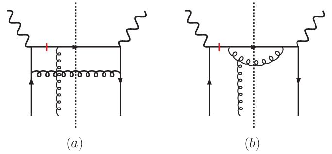
We are interested to obtain the differential cross section in the limit of $P_{\Lambda\perp}\ll Q$. In this limit, we further find that only $V_{4}$ and $V_{9}$ in Eq. (6) contribute in the leading power of $P_{\Lambda\perp}/Q$. $V_{4}$ and $V_{9}$ are defined as,

and the associated $\tilde{V}_{4}$ and $\tilde{V}_{9}$ are given by,

These two terms contribute the same to the differential cross sections except the azimuthal angular dependence. The contribution from $V_{4}$ is proportional to $\cos(2\phi_{\Lambda}^{l})\sin(\phi_{s}^{l}-\phi_{\Lambda}^{l})$, where $\phi^{l}_{\Lambda}$ and $\phi_{s}^{l}$ are the azimuthal angles of the transverse momentum $P_{\Lambda\perp}$ and the polarization vector $S_{\Lambda\perp}$ of $\Lambda$ relative to the lepton scattering plane. On the other hand, the $V_{9}$ contribution is proportional to $\sin(2\phi_{\Lambda}^{l})\cos(\phi_{s}^{l}-\phi_{\Lambda}^{l})$. The total contributions from these two terms will be proportional to $\sin(\phi_{\Lambda}^{l}+\phi_{s}^{l})$.

Summing up both soft-pole and hard-pole contributions from all the diagrams similar to those in Fig. 1, we obtain the following $\Lambda$ polarization dependent differential cross section from the contributions from $V_{4}$ and $V_{9}$,

where $\xi=x_{B}/x$ and $\hat{\xi}=z_{h}/z$. In the above result, the fist term in the bracket is the derivative term coming from the soft-gluon pole, the second term is the non-derivation contribution from soft-gluon pole, and the third is the hard-pole contribution whose derivative term vanishes.

In order to compare to the TMD factorization formalism, we will extrapolate our results into the region of $\Lambda_{QCD}\ll P_{h\perp}\ll Q$. In doing the expansion, we only keep the terms leading in $P_{h\perp}/Q$, and neglect all higher powers. For small $P_{h\perp}$, the delta function can be expanded as:

With this expansion,the spin-dependent cross section in the small $P_{h\perp}$ limit can be written as,

where

On the other side, the transverse-momentum-dependent factorization can be applied in the small $P_{h\perp}\ll Q$. Therefore one expects the above result can be reproduced in this approach. The $\Lambda$ polarization dependent cross section can be factorized as the following form [8, 9]

where $\hat{\vec{P}}_{\Lambda\perp}$ is the unit vector in direction of $\vec{P}_{\Lambda\perp}$, $h_{1,DIS}^{\perp}$ is the TMD Boer-Mulders function for DIS process, and $H_{1T}$ the TMD transversity fragmentation for $\Lambda$. $S(\lambda_{\perp})$ and $H_{UUT}(Q^{2})$ are the soft factor and hard factor, respectively. The simple integral symbol represents a complicated integral: $\int=\int d^{2}\vec{k}_{\perp}d^{2}\vec{p}_{\perp}d^{2}\vec{\lambda}_{\perp}\delta^{2}(z\vec{k_{\perp}}+\vec{p}_{\perp}+\vec{\lambda}_{\perp}-\vec{P}_{\Lambda\perp}).$ We have suppressed the sum over all flavors and factorization scale dependence in the parton distribution function and fragmentation function.

When the $k_{\perp}$ is of the order of $\Lambda_{QCD}$ , the TMD dependent parton distribution function are entirely non-perturbative objects. But in the region $\Lambda_{QCD}\ll k_{\perp}\ll Q$, the TMD factorization still hold and at the same time $k_{\perp}$ dependent parton distribution function $h_{1}^{\perp}$ can be calculated in terms of the twist-three parton correlation function within the perturbative QCD. This provides us a chance to make contact with the result from the collinear factorization formalism. The perturbative calculation follow the similar procedure as that in [18]. Finally, one obtains,

where $A$ is given in Eq.(19), and $\xi=x_{B}/x$. We note that the native-time-reversal-odd TMD Boer-Mulders function is process-dependent. The above result is for SIDIS. When we apply the above to the Drell-Yan process, the Boer-Mulders function shall change the sign. Similarly, for the TMD transversity fragmentation function, we have,

where $H_{1T}(z)$ is the integrated transversity quark fragmentation function defined in Eq. (8) and $\hat{\xi}=z_{h}/z$.

To obtain the final result, we let one of the transverse momentum $\vec{k}_{\perp},\vec{p}_{\perp},\vec{l}_{\perp}$ be of the order of $\vec{P}_{\perp}$ and the others are much smaller. After integrating the delta function, one has,

where we have used the relation, $T_{F}^{(\sigma)}(x,x)=-\int d^{2}k_{\perp}\frac{|k_{\perp}|^{2}}{M_{p}}h^{\perp}_{1,DIS}(x,k_{\perp}^{2})$ [7, 28]. Obviously, we reproduce the differential cross sections from the collinear factorization calculation.

This clearly demonstrates that in the intermediate transverse momentum region, the twist-three collinear factorization approach and the TMD factorization approach provide a unique picture for the $\Lambda$ polarization in the unpolarized semi-inclusive DIS process. This is because the observable we calculated above is the leading contribution in the limit of $P_{\Lambda\perp}/Q$, and the TMD factorization is valid [8, 9].

The extension to the $\Lambda$ polarization in hadronic scattering is straightforward. The diagrams will be similar to what have been calculated for the SSA in inclusive hadron production in $pp_{\uparrow}\to\pi X$ collisions [12]. We need to change the twist-three correlation function $T_{F}$ to our $T_{F}^{\sigma}$ and couple to the transverse polarized fragmentation function for $\Lambda$. Again, we will have contributions from quark-quark, and quark-gluon scattering channels. Similar to what we have calculated in the last section, we will have both derivative and non-derivative contributions. The derivative terms have been calculated in [22]. Using the same method as that in [12], we calculated the non-derivative terms. To our surprise, from these calculations, we find that the non-derivative terms vanish for $\Lambda$ polarization in hard partonic scattering processes. This indicates that the compact formula [12] containing both derivative and non-derivative contributions may not work in general, and shows a counter-example of the derivation of the compact formula in [15]. It will be interesting to further investigate the reason for this observation.

In summary, in this paper, we studied the $\Lambda$ polarization in the unpolarized semi-inclusive DIS and $pp$ collisions. In the SIDIS process, we compared the twist-three approach with the TMD factorization approach and found that they are consistent with each other at the intermediate transverse momentum region. The calculations in $pp$ collisions show an interesting pattern that there are only derivative terms contributions and the non-derivative terms vanish.

We have also calculated the large transverse momentum behavior for the naive time-reversal-odd Boer-Mulders quark distribution in the twist-three approach from the quark-gluon-antiquark correlation function in unpolarized nucleon. This result can be generalized to that in the Drell-Yan process. Because of T-odd effects, we will have an opposite sign between these two processes,

This distribution has a number of important applications in the Drell-Yan lepton azimuthal distribution in $pp$ scattering. For example, the $\cos 2\phi$ angular distribution has contribution from two Boer-Mulders functions from the incoming nucleons [24]. From our calculations above, we shall be able to study the large transverse momentum behavior for this $\cos 2\phi$ angular distribution. The extension to this will be carried out in a separate publication.

This work was supported in part by the U.S. Department of Energy under contract DE-AC02-05CH11231 and the National Natural Science Foundation of China under the approval No. 10525523. We are grateful to RIKEN, Brookhaven National Laboratory and the U.S. Department of Energy (contract number DE-AC02-98CH10886) for providing the facilities essential for the completion of this work. J.Z. is partially supported by China Scholarship Council.

References

- [1] G. Bunce et al., Phys. Rev. Lett. 36, 1113 (1976); K. J. Heller et al., Phys. Rev. Lett. 41, 607 (1978) [Erratum-ibid. 45, 1043 (1980)].
- [2] M. Anselmino, A. Efremov and E. Leader, Phys. Rept. 261, 1 (1995) [Erratum-ibid. 281, 399 (1997)]; Z. T. Liang and C. Boros, Int. J. Mod. Phys. A 15, 927 (2000); V. Barone, A. Drago and P. G. Ratcliffe, Phys. Rept. 359, 1 (2002).
- [3] J. W. Qiu and G. Sterman, Phys. Rev. Lett. 67, 2264 (1991); Nucl. Phys. B 378, 52 (1992).
- [4] S. J. Brodsky, D. S. Hwang and I. Schmidt, Phys. Lett. B 530, 99 (2002); Nucl. Phys. B 642, 344 (2002).
- [5] J. C. Collins, Phys. Lett. B 536, 43 (2002).
- [6] X. Ji and F. Yuan, Phys. Lett. B 543, 66 (2002); A. V. Belitsky, X. Ji and F. Yuan, Nucl. Phys. B 656, 165 (2003).
- [7] D. Boer, P. J. Mulders and F. Pijlman, Nucl. Phys. B 667, 201 (2003).
- [8] X. Ji, J. P. Ma and F. Yuan, Phys. Rev. D 71, 034005 (2005); Phys. Lett. B 597, 299 (2004).
- [9] J. C. Collins and A. Metz, Phys. Rev. Lett. 93, 252001 (2004).
- [10] A. V. Efremov and O. V. Teryaev, Sov. J. Nucl. Phys. 36, 140 (1982) [Yad. Fiz. 36, 242 (1982)]; A. V. Efremov and O. V. Teryaev, Phys. Lett. B 150, 383 (1985).
- [11] Y. Kanazawa and Y. Koike, Phys. Lett. B 478, 121 (2000); Phys. Rev. D 64, 034019 (2001).
- [12] C. Kouvaris, J. W. Qiu, W. Vogelsang and F. Yuan, Phys. Rev. D 74, 114013 (2006).
- [13] H. Eguchi, Y. Koike and K. Tanaka, Nucl. Phys. B 763, 198 (2007).
- [14] H. Eguchi, Y. Koike and K. Tanaka, Nucl. Phys. B 752, 1 (2006).
- [15] Y. Koike and K. Tanaka, Phys. Rev. D 76, 011502 (2007).
- [16] D. W. Sivers, Phys. Rev. D 43, 261 (1991).
- [17] M. Anselmino, M. Boglione and F. Murgia, Phys. Lett. B 362, 164 (1995); M. Anselmino and F. Murgia, Phys. Lett. B 442, 470 (1998); M. Anselmino, M. Boglione, U. D’Alesio, E. Leader and F. Murgia, Phys. Rev. D 71, 014002 (2005).
- [18] X. Ji, J. W. Qiu, W. Vogelsang and F. Yuan, Phys. Rev. Lett. 97, 082002 (2006); Phys. Rev. D 73, 094017 (2006); Phys. Lett. B 638, 178 (2006); Y. Koike, W. Vogelsang and F. Yuan, arXiv:0711.0636 [hep-ph].
- [19] W. G. D. Dharmaratna and G. R. Goldstein, Phys. Rev. D 53, 1073 (1996).
- [20] Z. T. Liang and C. Boros, Phys. Rev. Lett. 79, 3608 (1997); H. Dong and Z. T. Liang, Phys. Rev. D 70, 014019 (2004) [arXiv:hep-ph/0403041].
- [21] M. Anselmino, D. Boer, U. D’Alesio and F. Murgia, Phys. Rev. D 65, 114014 (2002).
- [22] Y. Kanazawa and Y. Koike, Phys. Rev. D 64, 034019 (2001); Y. Koike, AIP Conf. Proc. 675, 574 (2003).
- [23] D. Boer and P. J. Mulders, Phys. Rev. D 57, 5780 (1998).
- [24] D. Boer, Phys. Rev. D 60, 014012 (1999).
- [25] J. w. Qiu and G. Sterman, Nucl. Phys. B 353, 105 (1991); Nucl. Phys. B 353, 137 (1991).
- [26] R. Meng, F. I. Olness and D. E. Soper, Phys. Rev. D 54, 1919 (1996).
- [27] Y. Koike and J. Nagashima, Nucl. Phys. B 660, 269 (2003) [Erratum-ibid. B 742, 312 (2006)].
- [28] J. P. Ma and Q. Wang, Eur. Phys. J. C 37, 293 (2004).