The Hall conductance, topological quantum phase transition and the Diophantine equation on honeycomb lattice

Let us consider (9) in the momentum space. By performing the Fourier transformation of $\psi_{n,m}$ and $\phi_{n,m}$,

	$\displaystyle\psi_{n,m}=\sum_{k_{x},k_{y}}e^{ik_{x}n+ik_{y}m}u({\bm{k}}),$
	$\displaystyle\phi_{n,m}=\sum_{k_{x},k_{y}}e^{ik_{x}n+ik_{y}m}v({\bm{k}}),$		(10)

(9) becomes

$\displaystyle h({\bm{k}})\left[\begin{array}[]{c}u(k_{x},k_{y})\\ v(k_{x},k_{y})\end{array}\right]-t_{a}\sigma_{+}\left[\begin{array}[]{c}u(k_{x},k_{y}+\pi\Phi)\\ v(k_{x},k_{y}+\pi\Phi)\end{array}\right]-t_{a}\sigma_{-}\left[\begin{array}[]{c}u(k_{x},k_{y}-\pi\Phi)\\ v(k_{x},k_{y}-\pi\Phi)\end{array}\right]=E\left[\begin{array}[]{c}u({\bm{k}})\\ v({\bm{k}})\end{array}\right],$

where $h({\bm{k}})$ and $\sigma_{\pm}$ are given by

$\displaystyle h({\bm{k}})=\left[\begin{array}[]{cc}\xi&\Delta^{(0)}({\bm{k}})\\ \Delta^{(0)*}({\bm{k}})&-\xi\end{array}\right],\quad\Delta^{(0)}({\bm{k}})=-2e^{ik_{x}}\cos k_{y},$

and

$\displaystyle\sigma_{+}=\left[\begin{array}[]{cc}0&1\\ 0&0\end{array}\right],\quad\sigma_{-}=\left[\begin{array}[]{cc}0&0\\ 1&0\end{array}\right].$

When $t_{a}=0$, (III.1) reduces to

$\displaystyle h({\bm{k}})\left[\begin{array}[]{c}u^{(0)}({\bm{k}})\\ v^{(0)}({\bm{k}})\end{array}\right]=E\left[\begin{array}[]{c}u^{(0)}({\bm{k}})\\ v^{(0)}({\bm{k}})\end{array}\right],$

then the energies $E$ are found to be

$\displaystyle E=\pm\sqrt{\xi^{2}+4\cos^{2}k_{y}}(\equiv\pm E^{(0)}(k_{y})),$

(33)

and the eigen vector with the positive energy, $E=E^{(0)}(k_{y})$, is

$\displaystyle\left[\begin{array}[]{c}u^{(0)}_{+}({\bm{k}})\\ v^{(0)}_{+}({\bm{k}})\end{array}\right]=\frac{1}{\sqrt{2E^{(0)}(k_{y})(\xi+E^{(0)}(k_{y}))}}\left[\begin{array}[]{c}\xi+E^{(0)}(k_{y})\\ \Delta^{(0)*}({\bm{k}})\end{array}\right],$

and that with the negative one, $E=-E^{(0)}(k_{y})$, is

$\displaystyle\left[\begin{array}[]{c}u^{(0)}_{-}({\bm{k}})\\ v^{(0)}_{-}({\bm{k}})\end{array}\right]=\frac{1}{\sqrt{2E^{(0)}(k_{y})(\xi+E^{(0)}(k_{y}))}}\left[\begin{array}[]{c}-\Delta^{(0)}({\bm{k}})\\ \xi+E^{(0)}(k_{y})\end{array}\right].$

Here the staggered potential $\xi$ removes singularities in the energies, $\pm E^{(0)}(k_{y})$, and the eigen vectors at $k_{y}=\pm\pi/2$. It also remedies the singularity of ${\bm{A}}({\bm{k}})$ in (125) at $k_{y}=\pm\pi/2$. To solve (III.1) in perturbative expansions in powers of $t_{a}$, it is convenient to take the basis $(u({\bm{k}}),v({\bm{k}}))$ as

$\displaystyle\left[\begin{array}[]{c}u({\bm{k}})\\ v({\bm{k}})\end{array}\right]=\alpha({\bm{k}})\left[\begin{array}[]{c}u_{+}^{(0)}({\bm{k}})\\ v_{+}^{(0)}({\bm{k}})\end{array}\right]+\beta({\bm{k}})\left[\begin{array}[]{c}u_{-}^{(0)}({\bm{k}})\\ v_{-}^{(0)}({\bm{k}})\end{array}\right].$

Substituting this into (III.1) and multiplying $(u_{+}^{(0)*}({\bm{k}}),v_{+}^{(0)*}({\bm{k}}))$ to the both sides, we obtain

	$\displaystyle\left(E-E^{(0)}(k_{y}^{0}+\pi\Phi m)\right)\alpha_{m}(k_{x},k_{y}^{0})=$
	$\displaystyle-t_{a}\left[u_{+}^{(0)*}(k_{x},k_{y}^{0}+\pi\Phi m)v_{+}^{(0)}(k_{x},k_{y}^{0}+\pi\Phi(m+1))\right]\alpha_{m+1}(k_{x},k_{y}^{0})$
	$\displaystyle-t_{a}\left[u_{+}^{(0)*}(k_{x},k_{y}^{0}+\pi\Phi m)v_{-}^{(0)}(k_{x},k_{y}^{0}+\pi\Phi(m+1))\right]\beta_{m+1}(k_{x},k_{y}^{0})$
	$\displaystyle-t_{a}\left[v_{+}^{(0)*}(k_{x},k_{y}^{0}+\pi\Phi m)u_{+}^{(0)}(k_{x},k_{y}^{0}+\pi\Phi(m-1))\right]\alpha_{m-1}(k_{x},k_{y}^{0})$
	$\displaystyle-t_{a}\left[v_{+}^{(0)*}(k_{x},k_{y}^{0}+\pi\Phi m)u_{-}^{(0)}(k_{x},k_{y}^{0}+\pi\Phi(m-1))\right]\beta_{m-1}(k_{x},k_{y}^{0}),$		(51)

where $\alpha_{m}(k_{x},k_{y}^{0})$ and $\beta_{m}(k_{x},k_{y}^{0})$ are defined as

$\displaystyle\alpha_{m}(k_{x},k_{y}^{0})=\alpha(k_{x},k_{y}^{0}+\pi\Phi m),\quad\beta_{m}(k_{x},k_{y}^{0})=\beta(k_{x},k_{y}^{0}+\pi\Phi m),$

(52)

and $k_{y}^{0}$ satisfies $0\leq k_{y}^{0}<2\pi/q$. Here we have used the normalization conditions of the functions $(u_{+}^{(0)}({\bm{k}}),v_{+}^{(0)}({\bm{k}}))$ and $(u_{-}^{(0)}({\bm{k}}),v_{-}^{(0)}({\bm{k}}))$. In a similar manner, we also have

	$\displaystyle\left(E+E^{(0)}(k_{y}^{0}+\pi\Phi m)\right)\beta_{m}(k_{x},k_{y}^{0})=$
	$\displaystyle-t_{a}\left[u_{-}^{(0)*}(k_{x},k_{y}^{0}+\pi\Phi m)v_{+}^{(0)}(k_{x},k_{y}^{0}+\pi\Phi(m+1))\right]\alpha_{m+1}(k_{x},k_{y}^{0})$
	$\displaystyle-t_{a}\left[u_{-}^{(0)*}(k_{x},k_{y}^{0}+\pi\Phi m)v_{-}^{(0)}(k_{x},k_{y}^{0}+\pi\Phi(m+1))\right]\beta_{m+1}(k_{x},k_{y}^{0})$
	$\displaystyle-t_{a}\left[v_{-}^{(0)*}(k_{x},k_{y}^{0}+\pi\Phi m)u_{+}^{(0)}(k_{x},k_{y}^{0}+\pi\Phi(m-1))\right]\alpha_{m-1}(k_{x},k_{y}^{0})$
	$\displaystyle-t_{a}\left[v_{-}^{(0)*}(k_{x},k_{y}^{0}+\pi\Phi m)u_{-}^{(0)}(k_{x},k_{y}^{0}+\pi\Phi(m-1))\right]\beta_{m-1}(k_{x},k_{y}^{0}).$		(53)

When $t_{a}=0$, these equations reduce to

	$\displaystyle(E-E^{(0)}(k_{y}^{0}+\pi\Phi m))\alpha_{m}(k_{x},k_{y}^{0})=0,$
	$\displaystyle(E+E^{(0)}(k_{y}^{0}+\pi\Phi m))\beta_{m}(k_{x},k_{y}^{0})=0,$		(54)

and the unperturbed solutions are given by

$\displaystyle E=E^{(0)}(k_{y}^{0}+\pi\Phi m),\quad\alpha_{m}(k_{x},k_{y}^{0})=1,\quad\beta_{m}(k_{x},k_{y}^{0})=0,$

(55)

and

$\displaystyle E=-E^{(0)}(k_{y}^{0}+\pi\Phi m),\quad\alpha_{m}(k_{x},k_{y}^{0})=0,\quad\beta_{m}(k_{x},k_{y}^{0})=1,$

(56)

which reproduce (III.1) and (III.1), respectively. In the new basis, $\alpha({\bm{k}})$ and $\beta({\bm{k}})$ describe the upper $(E>0)$ and lower $(E<0)$ bands, respectively. The energy spectrum for $t_{a}=0$ is shown in Fig.3.

In (51) and (53), the terms proportional to $t_{a}$ give couplings between the momenta $k_{y}$ and $k_{y}\pm\pi\Phi$. So, if we put $\Phi=p/q$ with co-prime integers $p$ and $q$ $(q>0)$, then in general gaps open when $E^{(0)}(k_{y})=E^{(0)}(k_{y}^{\prime})$ with

$\displaystyle k_{y}=k_{y}^{\prime}+\pi\left(\frac{p}{q}\right)t,\quad k_{y}=-k_{y}^{\prime}+\pi s.$

(57)

Here $s$ is an integer, and $k_{y}$ and $k_{y}^{\prime}$ couple by $|t|$th-order perturbation. The size of the gap is an order of $t_{a}^{|t|}$. If $s$ is chosen appropriately, $k_{y}$ is put between $0$ and $\pi$ and $k_{y}$ for the $r$-th gap from the bottom can be chosen as

$\displaystyle k_{y}=\left(\frac{r}{2q}\right)\pi,$

(58)

where $r$ is an integer with $1\leq r\leq 2q-1$. (Gaps with $1\leq r\leq q-1$ open in the lower band $(E<0)$, and those with $q+1\leq r\leq 2q-1$ open in the upper band $(E>0)$. A gap at $E=0$ corresponds to $r=q$, but it closes when $\xi\rightarrow 0$ for a weak $t_{a}$.) Eliminating $k_{y}$ and $k_{y}^{\prime}$ from (57) and (58), we have the Diophantine equation

$\displaystyle r=qs_{r}+pt_{r},$

(59)

where we have written the subscript $r$ since $t$ and $s$ depend on $r$ implicitly as a solution of (59).

We can also derive the formula (3) in the perturbation theory. For brevity, we derive it only for gaps in the upper band ($E>0$). The same formula can be obtained for gaps in the lower band ($E<0$) in a similar manner. The wave function in the upper band ($E>0$) is simply given by

$\displaystyle\left[\begin{array}[]{c}u(k_{x},k_{y}^{0})\\ v(k_{x},k_{y}^{0})\end{array}\right]=\alpha_{m}(k_{x},k_{y}^{0})\left[\begin{array}[]{c}u_{+}^{(0)}(k_{x},k_{y}^{0}+\pi\phi m)\\ u_{-}^{(0)}(k_{x},k_{y}^{0}+\pi\phi m)\end{array}\right]+\alpha_{m^{\prime}}(k_{x},k_{y}^{0})\left[\begin{array}[]{c}u_{+}^{(0)}(k_{x},k_{y}^{0}+\pi\phi m^{\prime})\\ u_{-}^{(0)}(k_{x},k_{y}^{0}+\pi\phi m^{\prime})\end{array}\right],$

where $m=m^{\prime}+t$ and we take $0\leq k_{y}^{0}<\pi/q$. The gaps are at $k_{y}^{0}=0$ and $\pi/2q$. Write $\alpha_{m}=a$ and $\alpha_{m^{\prime}}=b$, then an effective Schrödinger equation is given by

$\displaystyle\left[\begin{array}[]{cc}\epsilon&\eta e^{ik_{x}t}\\ \eta e^{-ik_{x}t}&-\epsilon\end{array}\right]\left[\begin{array}[]{c}a\\ b\end{array}\right]=E\left[\begin{array}[]{c}a\\ b\end{array}\right],$

where $\epsilon$ and $E$ are measured from the middle of the gap, namely

$\displaystyle E=E^{(0)}(k_{y}^{0}+\pi\phi m),$

(74)

and $k_{y}^{0}=0$ for even $r$ or $\pi/2q$ for odd $r$. Here the $k_{x}$-dependence of the off diagonal elements of the matrix in (III.1) is determined by (III.1), (III.1) and (51), and the parameter $\eta$ is a real number and of the order of $t_{a}^{|t|}$. The solutions of (III.1) are

	$\displaystyle E_{+}=\sqrt{\epsilon^{2}+\eta^{2}},$
	$\displaystyle\left[\begin{array}[]{c}a_{+}\\ b_{+}\end{array}\right]=\frac{1}{\sqrt{2E_{+}(E_{+}-\epsilon)}}\left[\begin{array}[]{c}\eta\\ (E_{+}-\epsilon)e^{-ik_{x}t}\end{array}\right],$

and

	$\displaystyle E_{-}=-\sqrt{\epsilon^{2}+\eta^{2}},$
	$\displaystyle\left[\begin{array}[]{c}a_{-}\\ b_{-}\end{array}\right]=\frac{1}{\sqrt{2E_{-}(E_{-}-\epsilon)}}\left[\begin{array}[]{c}\eta\\ (E_{-}-\epsilon)e^{-ik_{x}t}\end{array}\right].$

When $\epsilon/|\eta|\rightarrow\infty$, these solutions behave as

$\displaystyle\left[\begin{array}[]{c}a_{+}\\ b_{+}\end{array}\right]\rightarrow\left[\begin{array}[]{c}{\rm sgn}\eta\\ 0\end{array}\right],\quad\left[\begin{array}[]{c}a_{-}\\ b_{-}\end{array}\right]\rightarrow\left[\begin{array}[]{c}0\\ -e^{-ik_{x}t}\end{array}\right],$

and when $\epsilon/|\eta|\rightarrow-\infty$,

$\displaystyle\left[\begin{array}[]{c}a_{+}\\ b_{+}\end{array}\right]\rightarrow\left[\begin{array}[]{c}0\\ e^{-ik_{x}t}\end{array}\right],\quad\left[\begin{array}[]{c}a_{-}\\ b_{-}\end{array}\right]\rightarrow\left[\begin{array}[]{c}{\rm sgn}\eta\\ 0\end{array}\right].$

For the upper edges of $r$-th band, we take the solution (III.1) with $t=t_{r}$. The asymptotic behaviors (III.1) and (III.1) imply that as $k_{y}^{0}$ passes $0$ (for even $r$) or $\pi/2q$ (for odd $r$), the wave function changes from

$\displaystyle\left[\begin{array}[]{c}u(k_{x},k_{y}^{0})\\ v(k_{x},k_{y}^{0})\end{array}\right]_{-}={\rm sgn}\eta\left[\begin{array}[]{c}u_{+}^{(0)}(k_{x},k_{y}^{0}+\pi\phi m)\\ u_{+}^{(0)}(k_{x},k_{y}^{0}+\pi\phi m)\end{array}\right]$

to

$\displaystyle\left[\begin{array}[]{c}u(k_{x},k_{y}^{0})\\ v(k_{x},k_{y}^{0})\end{array}\right]_{-}=-e^{-ik_{x}t_{r}}\left[\begin{array}[]{c}u_{+}^{(0)}(k_{x},k_{y}^{0}+\pi\phi m^{\prime})\\ u_{+}^{(0)}(k_{x},k_{y}^{0}+\pi\phi m^{\prime})\end{array}\right].$

And for the lower edge of $r$-th band, we take the solution (III.1) with $t=t_{r-1}$, then we have asymptotic behaviors of the wave function in a similar manner. On the overlap in the center of the band, these wave functions are related to each other by transition functions. See Fig.4. On the overlap ${\rm I}$ in Fig.4, the wave function (III.1) is identified with

$\displaystyle\left[\begin{array}[]{c}u(k_{x},k_{y}^{0})\\ v(k_{x},k_{y}^{0})\end{array}\right]_{+}={\rm sgn}\eta\left[\begin{array}[]{c}u_{+}^{(0)}(k_{x},k_{y}^{0}+\pi\phi m)\\ u_{+}^{(0)}(k_{x},k_{y}^{0}+\pi\phi m)\end{array}\right],$

by a trivial transition function, $e^{i\theta}=1$, and on the overlap ${\rm II}$, (III.1) is identified with

$\displaystyle\left[\begin{array}[]{c}u(k_{x},k_{y}^{0})\\ v(k_{x},k_{y}^{0})\end{array}\right]_{+}=e^{-ik_{x}t_{r-1}}\left[\begin{array}[]{c}u_{+}^{(0)}(k_{x},k_{y}^{0}+\pi\phi m^{\prime})\\ u_{+}^{(0)}(k_{x},k_{y}^{0}+\pi\phi m^{\prime})\end{array}\right],$

by the transition function

$\displaystyle e^{i\theta(k_{x})}=-e^{ik_{x}(t_{r}-t_{r-1})}.$

(123)

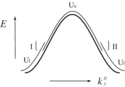
Now let us calculate the contribution of the $r$-th band to the Hall conductance,

$\displaystyle\sigma^{(r)}_{xy}$

$\displaystyle=$

$\displaystyle-\frac{e^{2}}{h}\frac{1}{2\pi}\int\int dk_{x}dk_{y}^{0}(\nabla_{\bm{k}}\times{\bm{A}}({\bm{k}}))_{z}.$

(124)

Here the integration of (124) is performed on the first magnetic Brillouin zone, and ${\bm{A}}({\bm{k}})$ is defined as

$\displaystyle{\bm{A}}({\bm{k}})=-i[u^{*}({\bm{k}})\nabla_{\bm{k}}u({\bm{k}})+v^{*}({\bm{k}})\nabla_{\bm{k}}v({\bm{k}})],$

(125)

where $(u({\bm{k}}),v({\bm{k}}))$ is the wave function for the $r$-th band constructed above. For the present purpose, it is convenient to consider the rectangle region given by $-\pi\leq k_{x}<\pi$ and $0\leq k_{y}^{0}<2\pi/q$, which is equivalent to a pair of the first magnetic Brillouin zone. Performing the integral (124) in this region and dividing it by 2, we have

$\displaystyle\sigma^{(r)}_{xy}=-\frac{e^{2}}{h}\frac{1}{4\pi}\int_{-\pi}^{\pi}dk_{x}\int_{0}^{2\pi/q}dk_{y}^{0}(\nabla_{\bm{k}}\times{\bm{A}}({\bm{k}}))_{z}.$

(126)

From the Stokes theorem, one can show that only the transition function (123) in the center of the band contributes to this integral. Thus we obtain

$\displaystyle\sigma^{(r)}_{xy}=-\frac{e^{2}}{h}\frac{1}{4\pi}\int_{-\pi}^{\pi}dk_{x}\partial_{x}\theta(k_{x})\times 2=-\frac{e^{2}}{h}(t_{r}-t_{r-1}).$

(127)

(The factor 2 arises because we have the transition function (123) twice in the integral region of (126).) When the Fermi surface is in the $r$-th gap from the bottom, we have the formula (3),

$\displaystyle\sigma_{xy}=\sum_{r^{\prime}=1}^{r}\sigma_{xy}^{(r^{\prime})}=-\frac{e^{2}}{h}t_{r}.$

(128)

Let us now determine the Hall conductance. As we showed above, the Hall conductance in units of $-e^{2}/h$, namely $t_{r}$, satisfies the Diophantine equation. By combining with the perturbation theory, the Diophantine equation enables us to determine the Hall conductance algebraically.

Before giving a rule to determine the Hall conductance, we briefly summarize properties of the Diophantine equation which we shall use later. First, the Diophantine equation has an infinite number of solutions: If we have a solution $(s_{r},t_{r})$ for a given $r$, then $(s_{r}-lp,t_{r}+lq)$ for any integer $l$ is also a solution. Second, the minimal value of $|t_{r}|$ among the solutions satisfies $|t_{r}|\leq q/2$. We denote a solution with the minimal $|t_{r}|$ by $(s_{r}^{0},t_{r}^{0})$. Third, except when $q$ is an even integer and $|t_{r}|=q/2$, $(s_{r}^{0},t_{r}^{0})$ is uniquely determined. When $|t_{r}|=q/2$, we have two solutions: $t_{r}^{0}=\pm q/2$.

As we denoted in Sec.III.1, $|t_{r}|$ is an order of the perturbation. So one naively expect that the size of the $r$th gap from the bottom and its Hall conductance are given by its minimal value $t_{r}^{0}$. But this is not always correct. The reason why is that if an intermediate state in the $|t_{r}^{0}|$th order perturbation has the momentum ${\bm{k}}$ with $\Delta^{(0)}({\bm{k}})=0$, (namely ${\bm{k}}$ with $k_{y}=\pi/2$ $(\mbox{mod $\pi$})$, then the transition amplitude becomes zero. For example, let us consider a gap at $k_{y}=(r/2q)\pi$ with $r=q+4p$. (We assume that $q\gg p$.)

In this case, the minimal value of $|t_{r}|$ is given by $t_{r}=4$, so a naive expectation is that the gap opens in fourth order perturbation. In Fig.5, we illustrate intermediate states. As is seen there, we have to pass through either $\alpha_{m-2}$ or $\beta_{m-2}$ as an intermediate state, and both of them have $k_{y}=\pi/2$. From (51) and (53), the transition amplitude to the intermediate state $\alpha_{m-2}$ is proportional to

$\displaystyle v_{+}^{(0)}(k_{x},k_{y}^{0}+\pi\Phi(m-2))\propto\Delta^{(0)*}(k_{x},\frac{\pi}{2}),$

(129)

and that from $\beta_{m-2}$ is proportional to

$\displaystyle u_{-}^{(0)*}(k_{x},k_{y}^{0}+\pi\Phi(m-2))\propto\Delta^{(0)*}(k_{x},\frac{\pi}{2}),$

(130)

and both of them are zero since $\Delta^{(0)}({\bm{k}})=0$ at $k_{y}=\pi/2$. So the matrix element between $\alpha_{m}$ and $\alpha_{m-4}$ vanishes. As a result, no gap opens in the fourth order perturbation. The gap opens in a higher order perturbation.

Now let us derive a condition that the transition amplitude in $|t_{r}^{0}|$th order perturbation vanishes. Without losing generality we can assume that $t_{r}^{0}\neq 0$ since $t_{r}^{0}$ becomes zero only for a gap at $E=0$, which closes when $\xi\rightarrow 0$. We also assume that $|t_{r}^{0}|\neq q/2$. The case of $|t_{r}^{0}|=q/2$ is discussed later. Consider the mixing between $k_{y}$ and $k_{y}^{\prime}$ with

$\displaystyle k_{y}=\left(\frac{r}{2q}\right)\pi,\quad k_{y}=k_{y}^{\prime}+\pi\left(\frac{p}{q}\right)t_{r}^{0},\quad k_{y}=-k_{y}^{\prime}+\pi s_{r}^{0}.$

(131)

There are $|t_{r}^{0}|-1$ intermediate states, and since $k_{x}$ and $k_{x}^{\prime}$ are given by

$\displaystyle k_{y}=\frac{\pi}{2}s_{r}^{0}+\frac{\pi}{2}\left(\frac{p}{q}\right)t_{r}^{0},\quad k_{y}^{\prime}=\frac{\pi}{2}s_{r}^{0}-\frac{\pi}{2}\left(\frac{p}{q}\right)t_{r}^{0},$

(132)

they have momenta

$\displaystyle k_{y}^{\prime\prime}=\frac{\pi}{2}s_{r}^{0}+\frac{\pi}{2}\left(\frac{p}{q}\right)(t_{r}^{0}-2l),$

(133)

where

$\displaystyle l=\left\{\begin{array}[]{ll}1,2,\cdots,t_{r}^{0}-1,&\mbox{for $t_{r}^{0}>0$},\\ -1,-2,\cdots,t_{r}^{0}+1,&\mbox{for $t_{r}^{0}<0$}.\end{array}\right.$

If $k_{y}^{\prime\prime}$ in (133) becomes $\pi/2$ $(\mbox{mod $\pi$})$, then the transition amplitude in the $|t_{r}^{0}|$th order perturbation vanishes. In order for $k_{y}^{\prime\prime}$ to be $\pi/2$ $(\mbox{mod $\pi$})$,

$\displaystyle\left(\frac{p}{q}\right)(t_{r}^{0}-2l)$

(137)

must be an integer at least. And to satisfy this $t_{r}^{0}-2l$ is needed to be a multiple of $q$ since $p$ and $q$ are co-prime integers. But because $t_{r}^{0}$ satisfies

$\displaystyle|t_{r}^{0}-2l|\leq|t_{r}|\leq\frac{q}{2},$

(138)

this is possible only when $t_{r}^{0}-2l=0$. Thus $t_{r}^{0}$ must be even. Furthermore, $s_{r}^{0}$ must be odd in order for $k_{y}^{\prime\prime}$ to be $\pi/2$ $(\mbox{mod $\pi$})$ since $k_{y}^{\prime\prime}=(\pi/2)s_{r}^{0}$ when $t_{r}^{0}=2l$. Therefore only when $t_{r}^{0}$ is an even integer and $s_{r}^{0}$ an odd one, the transition amplitude vanishes. Otherwise, we have a nonzero transition amplitude in the $|t_{r}^{0}|$th order perturbation in general.

When $t_{r}^{0}$ is an even integer and $s_{r}^{0}$ an odd one, a nonzero transition amplitude is obtained in the next leading order. The next minimum value of $|t_{r}|$ is given by

$\displaystyle t_{r}=\left\{\begin{array}[]{ll}t_{r}^{0}-q,&\mbox{for $t_{r}^{0}>0$},\\ t_{r}^{0}+q,&\mbox{for $t_{r}^{0}<0$}.\end{array}\right.$

The intermediate states in this order have momenta

	$\displaystyle k_{y}^{\prime\prime}$	$\displaystyle=$	$\displaystyle\frac{\pi}{2}s_{r}+\frac{\pi}{2}\left(\frac{p}{q}\right)(t_{r}-2l)$		(142)
		$\displaystyle=$	$\displaystyle\frac{\pi}{2}s_{r}^{0}+\frac{\pi}{2}\left(\frac{p}{q}\right)(t_{r}^{0}-2l)$

with $s_{r}=s_{r}^{0}+p$ $(s_{r}=s_{r}^{0}-p)$ for $t_{r}^{0}>0$ $(t_{r}^{0}<0)$ and

$\displaystyle l=\left\{\begin{array}[]{ll}-1,-2,\cdots,t_{r}^{0}-q+1,&\mbox{for $t_{r}^{0}>0$},\\ 1,2,\cdots,t_{r}^{0}+q-1,&\mbox{for $t_{r}^{0}<0$}.\end{array}\right.$

This $k_{y}^{\prime\prime}$ can not be $\pi/2$ $(\mbox{mod $\pi$})$: In order for $k_{y}^{\prime\prime}$ to be $\pi/2$ $(\mbox{mod $\pi$})$, $t_{r}^{0}/2-l$ must be a multiple of $q$, but this can not be met from the restriction $0<|t_{r}^{0}/2-l|<q$.

Now we summarize a procedure to determine the Hall conductance for the $r$th gap from below under a magnetic field $\Phi=p/q$.

1. 1.

   First, find a solution of the Diophantine equation, $(s_{r}^{0},t_{r}^{0})$, which satisfies $|t_{r}^{0}|\leq q/2$.

2. 2.

   Then if $t_{r}^{0}$ is an even integer and $s_{r}^{0}$ an odd one, the Hall conductance is given by

   $\displaystyle\sigma_{xy}=\left\{\begin{array}[]{ll}-\frac{e^{2}}{h}(t_{r}^{0}-q),&\mbox{for $t_{r}^{0}>0$},\\ -\frac{e^{2}}{h}(t_{r}^{0}+q),&\mbox{for $t_{r}^{0}<0$},\end{array}\right.$

   The size of the gap is an order $t_{a}^{q-|t_{r}^{0}|}$.

3. 3.

   For the other cases, the Hall conductance is given by

   $\displaystyle\sigma_{xy}=-\frac{e^{2}}{h}t_{r}^{0},$

   (149)

   and the size of the gap is an order of $t_{a}^{|t_{r}^{0}|}$.

Finally, let us discuss the case of $|t_{r}^{0}|=q/2$. This is possible only when $q$ is even and only for gaps with $r=q/2$ or $r=3q/2$. Although we have two solutions of the Diophantine equation, $t_{r}^{0}=\pm q/2$, the Hall conductance is determined uniquely if $q/2$ is an even integer. Since $p$ is odd when $q$ is even, it can be shown that one of these solutions has an odd $s_{r}^{0}$ and the other has an even $s_{r}^{0}$. So from the argument above, it is found that if $q/2$ is an even number, the solution with an odd $s_{r}^{0}$ has vanishing transition amplitude in the $(q/2)$-th perturbation. Thus the Hall conductance is given by the solution $t_{r}^{0}$ with an even $s_{r}^{0}$.

References

- [1] K. S. Novoselov, E. McCann, S. V. Morozov, V. I. Fal’ko, M. I. Katsnelson, V. Zeitler, D. Jiang, F. Schedin, and A. K. Gein, Nature 438, 197 (2005).
- [2] Y. Zhang, Y. W. Tan, H. L. Stormer, and P. Kim, Nature 438, 201 (2005).
- [3] V. P. Gusynin and S. G. Sharapov, Phys. Rev. Lett. 95, 146801 (2005).
- [4] Y. Zheng and T. Ando, Phys. Rev. B 65, 245420 (2002).
- [5] N. M. R. Peres, F. Guinea, and A. H. C. Neto, Phys. Rev. B 73, 125411 (2006).
- [6] K. S. Novoselov, E. McCann, S. V. Morozov, V. I. Fal’ko, M. I. Katsnelson, U. Zeitler, D. Jiang, F. Schedin, and A. K. Geim, Nat. Phys. 2, 177 (2006).
- [7] M. Oshikawa, Phys. Rev. B 50, 17357 (1994).
- [8] Y. Hatsugai, T. Fukui, and H. Aoki, Phys. Rev. B 74, 205414 (2006).
- [9] R. Rammal, J. Phy. (Paris) 46, 1345 (1985).
- [10] Y. Hasegawa and M. Kohmoto, Phys. Rev. B 74, 155415 (2006).
- [11] B. A. Bernevig, T. L. Hughes, S. C. Zhang, H. D. Chen, and C. Wu, Int. J. Mod. Phys. B 20, 3257 (2006).
- [12] Y. Hasegawa, R. Konno, H. Nakano, and M. Kohmoto, Phys. Rev. B 74, 033413 (2006).
- [13] P. Dietl, F. Piéchon, and G. Montambaux, Phys. Rev. Lett. 100, 236405 (2008).
- [14] A. H. MacDonald, Phys. Rev. B 29, 3057 (1984).
- [15] S. Aubry and G. André, Ann. Isr. Phys. Soc. 3, 133 (1980).
- [16] D. J. Thouless, M. Kohmoto, M. P. Nightingale, and M. den Nijs, Phys. Rev. Lett. 49, 405 (1982).
- [17] M. Kohmoto, J. Phys. Soc. Jpn. 61, 2645 (1992).
- [18] P. Středa, J. Phys. C 15, L717 (1982a).
- [19] P. Středa, J. Phys. C 15, L1299 (1982b).
- [20] M. Kohmoto, Ann, Phys. (N.Y.) 160, 343 (1985).
- [21] J. E. Avron, R. Seiler, and B. Simon, Phys. Rev. Lett. 51, 51 (1983).
- [22] M. Kohmoto, Phys. Rev. B 39, 11943 (1988).
- [23] B. I. Halperin, Phys. Rev. B 25, 2185 (1982).
- [24] Y. Hatsugai, Phys. Rev. B 48, 11851 (1993a).
- [25] Y. Hatsugai, Phys. Rev. Lett. 71, 3697 (1993b).
- [26] X.-L. Qi, Y.-S. Wu, and S.-C. Zhang, Phys. Rev. B 74, 085308 (2006).
- [27] Y. Zhang, Z. Jiang, M. S. Purewal, Y. W. Tan, M. Fazlollahi, J. D. Chudow, J. A. Jaszczak, H. L. Stormer, and P. Kim, Phys. Rev. Lett. 96, 136806 (2006).
- [28] Z. Jiang, Y. Zhang, H. L. Stormer, and P. Kim, Phys. Rev. Lett. 99, 106802 (2007).