Up-and-Down and the Percentile-Finding Problem \AuthorAssaf Peretz Oron \Year2007
Statistics
A dissertation
submitted in partial fulfillment of
the requirements for the degree of
\ChairPeter D. HoffAssociate ProfessorStatistics
\SignaturePeter D. Hoff \SignaturePaul D. Sampson \SignatureBarry E. Storer \signaturepage
\doctoralabstractquoteslip
Up-and-Down (U&D), a popular sequential design for estimating threshold percentiles in binary experiments, has not been a major subject of statistical research since the 1960’s. U&D application practices have stagnated, and significant gaps in understanding its properties persist. The first part of my work aims to fill critical gaps in U&D theory. All U&D variants studied generate Markov chains of treatments. New results concerning stationary distribution properties are proven. A commonly used U&D variant known as “fixed forced-choice staircase” or “k-in-a-row” (KR), is proven to have a single-mode stationary distribution – contradicting recent remarks about it in literature. Moreover, KR is shown to be the best-performing design in terms of convergence rate and estimation precision, compared with other designs targeting the same percentiles. A second focus of this study is nonparametric U&D estimation. An improvement to isotonic regression called “centered isotonic regression” (CIR), and a new averaging estimator called “auto-detect” are introduced and their properties studied. Interval estimation solutions are also developed for both estimators.
Bayesian percentile-finding designs, most notably the continual reassessment method (CRM) developed for Phase I clinical trials, are also studied. CRM is believed to converge to exclusive allocation to a single optimal level, but to date, this belief had not been substantiated by extensive proofs. Here I add several proofs, expanding the understanding of when CRM might converge. In general, CRM convergence depends upon random run-time conditions – meaning that convergence is not always assured. Small-sample behavior is studied as well. It is shown that CRM is quite sensitive to outlier sub-sequences of thresholds, resulting in highly variable small-sample behavior between runs under identical conditions. Nonparametric CRM variants exhibit a similar sensitivity.
Ideas to combine the advantages of U&D and Bayesian designs are examined. A new approach is developed, using a hybrid framework, that evaluates the evidence for overriding the U&D allocation with a Bayesian one. This new design, called “Bayesian Up-and-Down” (BUD), is shown numerically to be more robust than CRM, and moderately outperforms either CRM or U&D in terms of estimation.
Acknowledgements.
This work started out in fall 2003 as a routine consulting task at the University of Washington Departments of Statistics’ consulting service, headed by Paul D. Sampson. I thank Prof. Sampson, the consulting client Dr. M.J. Souter (who approached us with the idea of using Up-and-Down for his experiment), consulting team leader Nancy Temkin of the Biostatistics department, and colleague David Dailey for arousing my initial interest and curiosity regarding the Up-and-Down design. During 2004 I was able to continue working on Up-and-Down and support Dr. Souter’s anesthesiology experiment, thanks to the work’s designation as a dependent data (“stochastic”) preliminary exam project, under the guidance of Prof. Sampson. Profs. Galen Shorack and Matthew Stephens were members of the exam committee. In summer 2005 I decided to turn the project into my dissertation, even though I was working with my advisor, Prof. Peter Hoff, on a rather different topic at the time. I thank Prof. Hoff and graduate coordinator Prof. Jon Wellner for the openness and flexibility they showed in supporting the transition. Thanks to my full doctoral committee - Profs. Hoff, Sampson, Wellner, GSR Nancy K. Rivenburgh of Communications and Margaret O’Sullivan Pepe and Barry E. Storer of Biostatistics and the Fred Hutchinson Cancer Research Center. Thanks to Marloes Maathuis who provided valuable and patient help with isotonic regression theory. Finally, thanks to my fellow students – especially to my study pal Veronica Berrocal – and to department staff, who were there to lend a helping hand along the way. Former graduate student advisor, the late Kristin Sprague (1947-2006), is fondly remembered. \dedicationTo the memory of my grandparents Lotte Lieberman-Oppenheim (1908-1989) Julius Oppenheim (1904-1993) Esther Berger-Hochman (1904-1980) Yehoshua-Shiyye Hochman (1906-2005) and my step-grandmother Mania Kalmanovich-Hochman (1917-2007) To my parents Rachel and Moshé Oron and parents-in-law Bat Sheva and Shimon Eliyahu, and most of all to my wife Orna Eliyahu-Oron and sons Daniel, Guy and Ben, who have tolerated and supported me through this journey. \textpagesChapter 1 Preface and Introduction
1.1 Preface
In many binary-response experiments, researchers are not interested in finding the entire treatment-response curve, but only a single representative value, which can be described via a percentile of the underlying threshold distribution . This percentile can represent (for example) the sensory threshold, the of a toxic substance, or the maximum-tolerated-dose (MTD) of a medication. Such experiments are typically limited to a sample of several dozen trials or even less, and with little prior knowledge about the form of . An additional, rather common constraint is that treatment levels are limited to a fixed, discrete, finitely-spaced set.
Statisticians have been developing designs to answer this type of challenge for at least two generations. Yet, interestingly, if an applied researcher were to seek statistical consulting on this problem, he or she would receive wildly differing recommendations, depending upon which field they work in or which statistician happened to be the consultant. Moreover, an applied statistician wishing to consult a client on this issue would discover, upon a cursory literature search, that any clear, well-tested and practical guidelines (if they exist) are drowning in a sea of contradictory “best practices” recommendations, antiquated references, unverified claims and controversy. In short: until quite recently, there was no up-to-date, standard reference for this problem.11 1 Apparently, I am not the only person to have noticed this. Chevret (2006) is a recent attempt to fill the gap. Pace and Stylianou (2007)’s review is an attempt to update the anesthesiology community with recent statistical developments relevant to their needs.
These are not hypothetical statements; this is exactly what happened to me in late 2003, when I was enlisted to help Dr. M. J. Souter design an anesthesiology percentile-finding experiment (Oron, 2004; Bhananker et al., 2007). My search for solid and reliable solutions has evolved into the dissertation you are reading. After this tortuous journey, I find it important to repeat in this introduction a well-known truism, which is somehow forgotten in this field’s prevalent patterns of debate. Here it is, in the form of a disclaimer:
Constrained by the binary response, a small sample size, an unknown response threshold distribution and a discrete treatment set, the quality of information the experiment can provide is limited. Failed experiments (however one chooses to define ”failure”) are far from unlikely. The degree of confidence expressed by many statisticians promoting this or that method is exaggerated.22 2 Fisher (2007), in a recent Anesthesiology editorial, voiced similar concerns regarding the use of ‘Up-and-Down’ methods.
Keeping this perspective in mind, there is quite enough room for theoretical insight and methodological developments. The next section will expand and clarify these statements.
1.2 Introduction
1.2.1 Conceptual Framework
As the opening paragraph explains, we are looking for a treatment value that will generate positive response with probability . We assume that this probability is monotone increasing in . Furthermore, we assume that the response is deterministically triggered via an underlying population (sub)distribution of response thresholds , with a density .33 3 This last assumption is often wrong, especially in psychophysical experiments to find the sensory threshold of a single subject. In that field, it is common to apply fixes such as added parameters for the false positive and false negative rates. However, the simplifying assumption allows us to treat and as one and the same, and focus on the core features of the problem. We aim to estimate , known as the target percentile, or simply the target.
An excellent, perhaps ideal experiment, would be to directly sample the thresholds themselves, . If this is possible, then without knowledge of a good target estimate would be , the sample -th order statistic (or -th percentile). For large , is approximately normal with asymptotic variance
| (1.1) |
This can be perceived as a rough precision benchmark for the percentile-finding problem.
Our conditions, however, are far from ideal. Rather than the thresholds themselves, we observe binary responses that can be interpreted as censored current-status information: at a given trial indexed with treatment , we know that if the response was ‘yes’ and if it was ‘no’. If we pool all our treatments to the same value , we can estimate with variance . This is not a very impressive feat; for example, unless is close to or , we need to get a CI of for . And the best we can achieve this way, is knowing whether , , or (if we are lucky) . It is no wonder that in the related problem of binary-response opinion polls (which are analogous to estimating at a single specified ), the minimal acceptable sample size is several hundred.
If we try to cover a larger range of treatments by splitting the sample equally between levels , we will obtain even less precise point estimates, with many observations taken quite far from – indicating a waste of resources. The MLE with no knowledge of ’s shape is not much more than an interpolation between these rather blunt point estimates (this is examined more closely in Chapter 3). Taking the range-covering approach further, if we could let vary randomly and continuously, the nonparametric MLE of for current-status data converges – both globally and locally – only at an rate (Kim and Pollard, 1990; Groenenboom and Wellner, 1992).
In short, the problem’s properties imply that our prospects for solidly successful target estimation are not very promising.
A way out of this quagmire would be some “intelligent” sequential scheme, that would lead us to collect most of our information in the vicinity of -- even though before our first trial we have little knowledge where that target might be -- and then allow for reasonably useful estimation.44 4 Observing (1.1), the concentration of observations around target is tantamount to artificially increasing – with a linear effect on estimation error. Again, as hinted previously, statisticians and others have suggested many such schemes, but the most widely used methods fall almost exclusively into one of two groups. These are Markovian or Up-and-Down (U&D) designs, and Bayesian schemes.
I shall revisit this generic sampling perspective occasionally throughout the dissertation.55 5 See Sections 2.2.1,3.2.1,4.2.5, 4.3.1 and 5.3.1. To complete this bird’s-eye view of the dissertation, I also suggest Section 3.6 – which summarizes my U&D-related findings in the form of practical recommendations – and the conclusions. Typically, these will also be the only places where the response threshold distribution might be referred to as . Otherwise, because of the threshold-triggering assumption spelled out above, I will refer to the threshold CDF as : an (indirect) function of treatments.
1.2.2 Some Definitions and Constraints
Before we proceed further, it may be a good idea to define the two design approaches. The following definition is broad enough to include all methods discussed in the thesis, and is in the spirit of Storer (2001); Potter (2002) and Ivanova and Flournoy (2006).
Definition 1
(i) An ‘Up-and-Down’ (U&D) or algorithm-based design is any percentile-finding, binary-response sequential experimental design with treatments and responses , respectively; with fixed, discrete treatment levels and sequential treatment allocation rules, which are functions of and possibly also , a set of fixed parameters.
(ii) A Bayesian or model-based scheme is as in (i) above, but the allocation rules are functions of , and a statistical model , where is a set of data-estimable parameters.
As Definition 1 indicates, the dissertation will only deal with designs constrained to a fixed discrete set . This excludes methods such as stochastic approximation and its descendants (Robbins and Monro, 1951; Lai, 2003). Additionally, we will usually assume that is evenly spaced (whether on the original or on a transformed scale), with level spacing .66 6 In some cases we will assume is finite and in others not, depending upon context. Usually the difference between the two cases is more notational than substantial. Other simplifying assumptions are that the underlying threshold CDF is continuous strictly increasing, that it has a density , and that thresholds in the experiment’s trials are i.i.d. draws from .
These assumptions will save a great deal of burdensome notation, and should help us focus on essential design and estimation properties rather than on terminology.77 7 Most results discussed here can be easily extended to cases when one suspects to behave otherwise, or wishes to run the experiment on an unevenly spaced .
1.2.3 Audience and Scope
Percentile-finding is an application encountered in many research fields. However, two fields have dominated the design debate. In one of them (psychophysics or sensory studies), it is because the field’s most routine experiment - determination of sensory thresholds - is modeled as a percentile-finding problem. Proper treatment of the sheer wealth and breadth of percentile-finding designs used in psychophysics may take several books. Fortunately, the constraints outlined above already filter out a large part of these designs.
The second field (Phase I clinical trials) is dominant not so much because of its prevalence, or because of the wealth of designs. In fact, the vast majority of Phase I trials still appear to use conservative protocols, which most statisticians (myself included) view as outdated. The ‘Phase I’ application has dominated debate mostly because of the large amount of resources and statistical attention commanded by clinical trials in general.
The typical practical constraints in these two fields are very different. In psychophysics, most experimental runs are carried out on a single subject. Sample size and trial cost are usually not a problem, and in principle the treatment can vary continuously (though most designs prefer to stick to a discrete set). The sensory threshold itself is also defined quite flexibly: anything from the median to the th percentile may be commonly encountered. By contrast, Phase I trials are limited to small sample size (), and are usually carried out in cohorts of patients. The target is typically between the th and rd percentile, and due to toxicity concerns it is preferably approached from below.
In between, the “vanilla” engineering and scientific applications are usually median-targeting, size-constrained, and for lack of statistical attention have continued to plough along with 1940’s to 1960’s methodology. The three application types are summarized in Table 1.1.
| Application | Psychophysics | Phase I | General Engineering |
|---|---|---|---|
| Target | Median or above | th to rd Percentile | Median |
| Cohort Size | 1 | 2 – 6 | 1 |
| Major Constraints | Simplicity, response fatigue/reliability | Toxicity, medical ethics, volunteers, duration | Simplicity, cost, duration, toxicity (in some cases) |
| Currently Popular Designs | A large variety, including U&D and Bayesian designs | ‘3+3’ protocol, with Bayesian designs increasingly popular | U&D |
My approach has been to steer clear of complete commitment to a single field’s specific needs. The rationale is that this is precisely a statistical researcher’s role: to look at the generic problem, examine and formulate solutions to it - solutions useful for all applications. From these generic solutions, it should not be difficult to tailor specific applications. All that being said, given the medical motivation that introduced me to the problem, the terms and concerns encountered in medical literature are more prevalent in this thesis than those of other fields.
1.2.4 Thesis Layout
The thesis focuses on the most veteran family of U&D designs, which includes the original 1940’s method (Dixon and Mood, 1948). Chapter 2 tackles the designs themselves, while Chapter 3 is devoted to estimation. In recent decades, Bayesian model-based designs known under acronyms such as QUEST and CRM (Watson and Pelli, 1983; O’Quigley et al., 1990) have quickly eclipsed U&D in the number of statisticians studying them (though not in their prevalence of use). These designs are discussed in Chapter 4. There have been some attempts to combine the two approaches, and I have devoted quite a bit of energy to this as well. Combined approaches are discussed in Chapter 5, which is followed by the conclusions. To minimize confusion between the thesis terminology and that of other publications, I will refer to the algorithm-based design family simply as U&D, and to the model-based family as CRM or “Bayesian”.
Rather than precede the thesis body with a long and tedious introduction to all these subjects, I have opted to start each chapter with an introductory section, which reviews the current state of knowledge on that chapter’s topic. Such sections are followed by sections with theoretical results, and then sections with new methodological developments. In Chapter 3, the dissertation’s largest chapter, there is also a separate section presenting numerical results 88 8 In other chapters, numerical results are embedded within the sections., a section reporting and analyzing the results of the motivating anesthesiology experiment, which has been recently completed (Bhananker et al., 2007) – and finally, a section summarizing Chapters 2-3 with a list of practical recommendations. At the end of Chapters 2, 3 and 4 the reader can find glossaries for these chapters.
1.2.5 The Role of Simulation
In fall 2003, while still on the anesthesiology consulting job, team leader Nancy Temkin suggested that I use computer simulation to see how different U&D designs pan out. I proceeded to do so, unwittingly following in the footsteps of Wetherill, who in the 1960’s traveled across the ocean to make use of computing resources not available at the time in Great Britain (Wetherill, 1963; Wetherill et al., 1966). This was such a novelty back in England, that the mere use of simulations became a major gossip topic during the customary Royal Society discussion appearing in Wetherill (1963). Ever since then, for better or worse, simulation has played a central role in evaluating percentile-finding designs and estimators. Sometimes this approach is taken to the extreme: recently, O’Quigley and Zohar (2006) in their mini-review of CRM claimed that numerical simulation should be the main approach in studying and evaluating designs for the small-sample percentile-finding problem.
I could not disagree more.
At their best, simulations can perform a role analogous to that of lab experiments – proving or disproving a theory, demonstrating a theoretical result, and revealing novel patterns that inspire further theoretical research. Much of the painstaking work carried out by García-Perez and colleagues over a decade, examining percentile-finding designs in psychophysics, belongs to this category (Garcìa-Perez, 1998; Alcalà-Quintana and Garcìa-Perez, 2004; Garcìa-Perez and Alcalà-Quintana, 2005).
Not at their best, simulations can be a lazy man’s escape from doing theory, producing individual trees that are then mistaken for a forest. A classic example is Wetherill’s “reversal” estimator (see Chapter 3), chosen in a large part because of favorable simulation outcomes (Wetherill et al., 1966). As Section 3.2 will show, in general this estimator is in fact inferior.
At their worst, simulations can be abused to further irrelevant agendas. Here the classic example is the rise of Bayesian designs for Phase I trials. Researchers have used simulations to “prove” this approach’s advantage over others, most notably U&D (O’Quigley and Chevret, 1991; Babb et al., 1998). Immediately upon presenting the first such simulation study, the authors openly called upon regulatory authorities to discontinue use of U&D (O’Quigley and Chevret, 1991). While this call was not heeded, such simulations and the confidence with which they were presented have doubtlessly played a role in shutting most of the statistical world off to U&D. But in both cases the comparisons have been “rigged” in several ways against U&D (see section 4.1 for details). More neutral comparisons (Garcìa-Perez and Alcalà-Quintana, 2005) have yielded an almost diametrically opposite conclusion. I hope this thesis would help explain why.
During my work on this problem, I have spent thousands of human and CPU hours on simulation. I tried to keep simulations “at their best” as defined above. Many times I have found myself to be lazy, discovering that months of simulations have saved me… minutes of theory. I have been quite wary, and hopefully have succeeded, in keeping myself from abusing simulations, as happened in the cases mentioned above.
As the thesis materialized, I have tended to base more and more of my results on theory and not on simulation. This has been a mostly successful endeavor. Simulation in this thesis is confined mainly to illustrating the pros and cons of different designs and point estimators under different scenarios, or for such essential technical tasks as evaluating the coverage of interval estimators. There are one or two exceptions, where the numerical pattern strongly suggests a theoretical result, but my quest for that result has been incomplete (U&D convergence comparison in Section 2.2, smoothed isotonic regression in Chapter 3). Here I have to cling to the well-worn, job-security cliché: hopefully future work will find that proof.
Chapter 2 The Up-and-Down Design and Some Variants
2.1 Description and Current Knowledge
2.1.1 Basic Terminology
Let be some experimental treatment with a binary response . We assume is continuous and strictly increasing. Researchers look for , the -th percentile (or -th quantile) of . Treatments are administered sequentially: both treatments and responses are indexed . Following trial , the next treatment is determined by some subset of all previous treatments and responses , and by the specific method’s transition rules. In U&D methods, experimental treatments are restricted to a fixed set of levels , with level spacing .11 1 However, since is continuous, we shall sometimes refer to as a continuous variable when studying properties of . The subsequent discussion focuses on targets at or below the median, but all results can be trivially translated to targets above the median.
2.1.2 History
The up-and-down (U&D) sequential method was developed in the 1940’s (Dixon and Mood, 1948; von Bekesy, 1947; Anderson et al., 1946). It is designed to estimate the median threshold, under constraints of moderate sample size and a discrete set of treatment levels. It is still in use today in its original applications - finding the median sensitivity of explosives to shock loading (Chao and Fuh, 2003) and estimating sensory thresholds (Treutwein, 1995; Garcìa-Perez, 1998). It can also be found in a wide array of applied research fields - including fatigue testing in metallurgy and material science (Lagoda and Sonsino, 2004), testing of dental restorative materials (Scherrer et al., 2003), breakdown voltage estimation in electrical engineering (Komori and Hirose, 2000), animal toxicity response (Sunderam et al., 2004), and anesthesiology (Capogna et al., 2001; Drover et al., 2004). In numerous applications, U&D is considered a standard method (JSME, 1981; ASTM, 1991; OECD, 1998; NIEHS, 2001). Note on terminology: the term “up-and-down” used to refer only to the median-finding design, but hereafter I shall use it in its more recent interpretation - any percentile-finding design that can be seen as an extension of the original method. That original method will be called ‘simple up-and-down’ (SU&D).
Methodological research during U&D’s early years (Brownlee et al., 1953; Derman, 1957; Wetherill, 1963; Dixon, 1965; Wetherill et al., 1966; Tsutakawa, 1967b) generated accepted practices for design and estimation. The first proper identification of the U&D treatment sequence as a Markov chain is credited to Tsutakawa (1967a); Tsutakawa (1967b). Paradoxically, just as this discovery was made, and as U&D was proliferating into more and more fields, statistical interest in the method had begun to dwindle. From the mid-1970’s until the late 1980’s, very few U&D theoretical or methodological studies were published. This gap has probably contributed to the rather uneven pattern of usage observed today. Different fields adhere to different practices, whose rationale has often been lost in the mists of time.
Sample size is a case in point. Dixon and Mood (1948) originally recommended a sample size of for median estimation. Shortly afterwards, there was a trend to tailor the method for smaller and smaller sample sizes, (Brownlee et al., 1953; Dixon, 1965). Nowadays, some military industries still use for median-sensitivity estimation (H. Dror, personal communication, 2006). Some groups in anesthesiology use a fixed sample size of for ED estimation (Capogna et al., 2001; Camorcia et al., 2004). In the same field, Paul and Fisher (2001) report that many anesthesiologists use the fourth reversal as a stopping rule – roughly equivalent to a dozen treatments (reversals will be defined later in this section). Meanwhile, many researchers in anesthesiology and elsewhere use for the same goal (Lichtman, 1998; Sunderam et al., 2004; Drover et al., 2004).
Since around 1990, methodological interest in U&D has been gradually picking up again. Practitioners in fields using U&D have expressed increased interest and skepticism about the method, leading to extensive studies – typically numerical – and to ad-hoc improvement suggestions (Garcìa-Perez, 1998; Zhang and Kececioglu, 1998; Braam and van der Zwaag, 1998; Lin et al., 2001; Paul and Fisher, 2001; Pollak et al., 2006). Several statistical teams have entered the fray as well, mostly in the context of Phase I clinical trials, which target the 20th to 33rd percentiles (Storer, 1989). This recent research has yielded results that incorporate advances in the study of Markov chains (Durham and Flournoy, 1994; Durham and Flournoy, 1995; Durham et al., 1995; Gezmu, 1996; Giovagnoli and Pintacuda, 1998; Ivanova et al., 2003; Bortot and Giovagnoli, 2005; Gezmu and Flournoy, 2006) and in estimation (Komori and Hirose, 2000; Chao and Fuh, 2001; Stylianou and Flournoy, 2002; Stylianou et al., 2003). Much of this progress is summarized by Ivanova and Flournoy (2006) and Pace and Stylianou (2007). All the same, some of the U&D’s basic properties are still seldom discussed.
But perhaps before everything else, the simple question of which U&D variant to choose for a given application, especially for non-median targets, has not been properly addressed. Since the 1950’s researchers have creatively proposed many dozens of non-median U&D variants (e.g., Wetherill et al. (1966); Storer (1989); Durham et al. (1995); Garcìa-Perez (1998); Ivanova et al. (2003); Bortot and Giovagnoli (2005)). Yet, only a handful of articles actually compare different U&D methods’ performance, and usually only via limited-scope simulations.22 2 The only exception that comes to mind is (Bortot and Giovagnoli, 2005), who prove that BCD is optimal among first-order Markovian methods. But applied researchers do not care about a method’s Markov-chain order; they would like to know which method is best for estimating a given percentile, under certain practical constraints. There are also many innovative non-U&D sequential designs to achieve the same goal (O’Quigley et al., 1990; Rosenberger and Grill, 1997), and one may legitimately question whether U&D is the best platform. But a comparison of U&D with other approaches means little, if the U&D design and estimation methods used are clearly inferior to other available U&D methods, of which the researchers were not aware.
Another interesting aspect of the historical gap in U&D research is the method’s perceived nature. U&D was originally tied to a parametric assumption: the thresholds were assumed to be normally distributed (Dixon and Mood, 1948; Dixon, 1965). Nowadays U&D is almost universally seen as a nonparametric design. There has been little theoretical exploration into the ramifications of this change in perception, regarding design and estimation as actually practiced in the field.
2.1.3 Transition Probabilities, Balance Equations and Stationary Formulae
The original, median-targeting simple up-and-down (SU&D) starts at an arbitrary level, and then moves up or down level, following ‘no’ or ‘yes’ responses, respectively. This makes SU&D a lattice random walk, with ‘up’ and ‘down’ transition probabilities and , respectively.33 3 On the boundaries, trivial “reflecting” conditions are imposed; this type of boundary conditions is assumed throughout the text, but explicit boundary details are omitted for brevity. Assuming , there is a stationary distribution (Tsutakawa, 1967b; Durham and Flournoy, 1995), obeying:
| (2.1) |
with straightforward normalization to determine . The symbol , hereafter termed “the stationary distribution profile”, is monotone decreasing in . Therefore, the stationary distribution has a single mode, including the possibility that the mode is on a boundary (Durham and Flournoy, 1995). The U&D treatment sequence is known as a random walk with a central tendency (see e.g., Hughes, 1995, Ch. 3.4). Durham and Flournoy (1994) prove that the stationary mode is at most one spacing interval away from the median.
This is the place to note that U&D’s basic properties, such as a single mode near target, are retained even under an infinite (unbounded) set of treatment levels. Since the profiles are monotone decreasing, with reference to the frequency at the mode the stationary frequencies form a sequence that decreases in a faster-than-geometric rate to either direction. Therefore, the overall sum of frequencies is a convergent series, even if carried to infinity, and always exists with a mode near target. Hence, distinguishing between a bounded set of treatments indexed , and an unbounded one indexed presents only a minor technical challenge and not a conceptual difference. Furthermore, as will be seen in Chapter 3, in some sense the unbounded-design version of U&D is the “pure” one.
Derman (1957) suggested modifying U&D via randomization in order to target non-median percentiles. However, the method now known as ‘biased-coin’ design (BCD) was developed independently by Durham and Flournoy (1994); Durham and Flournoy (1995). It is similar to SU&D, except that after a ‘no’ response the next treatment is determined using a random draw: with probability we go up one level, otherwise the level is unchanged (). Now , the probability of remaining at the same level for another trial, can be nonzero. The resulting transition probability rule as a function of is
| (2.2) |
The stationary distribution obeys (Durham and Flournoy, 1995)
| (2.3) |
Again, the walk has a central tendency and a single mode; it was shown (Durham and Flournoy, 1994) that the stationary mode is at most one spacing interval away from , which is the method’s designated target.
Another non-median U&D method is known as “forced-choice fixed staircase” or ‘k-in-a-row’ (KR) (Wetherill et al., 1966; Gezmu, 1996).44 4 In fairness, I should have used the term ‘staircase’ to refer to this method, since this is how most of its users (in psychophysics) know it. However, ‘k-in-a-row’ is shorter and more descriptive. Moreover, rigorously speaking, all U&D ‘flavors’ discussed here answer the definition ‘forced-choice fixed staircase’ (as contrasted with ‘adaptive staircase’, in which the ‘up’ and ‘down’ steps have different level spacing; see e.g. Garcìa-Perez (1998)). Here there is no random draw; instead, we must observe exactly consecutive ‘no’s at a given level before moving up (the ‘down’ rule remains as in SU&D). For , KR reduces to SU&D. Even though KR is by far the most widely used non-median U&D method and is arguably easier to administer than BCD (requiring no random draw), its Markov chain properties are more complex and have rarely been studied. KR’s transition probability matrix and stationary distribution were described by Gezmu in her unpublished dissertation (Gezmu, 1996). In numerical runs, KR has repeatedly exhibited advantages over similar-targeted BCD designs (Storer, 1989; Ivanova et al., 2003, see also). However, Gezmu and her collaborators have come to doubt the method’s theoretical properties, most notably the existence of a single stationary mode (Ivanova and Flournoy, 2006). This and other properties will be explored in the next section.
One aspect of KR that has been known since its inception (Wetherill et al., 1966) is its target: it is the solution to the equation 55 5 Paradoxically, Wetherill et al. (1966) derived KR’s target in an erroneous way: they calculated the target of a GU&D method to be presented below, and attributed it to KR.
| (2.4) |
Unlike BCD, KR can target only a discrete set of percentiles; for these are approximately and , respectively.66 6 In sensory studies the method is inverted: one ‘no’ response triggers an ‘up’ move, while consecutive ‘yes’ responses are required for a ‘down’ move. Hence the targets are , etc.
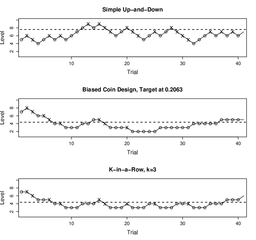
SU&D, BCD () and KR () are illustrated in Fig. 2.1 - where all three were run numerically on the same set of thresholds. As the figure shows, how closely an individual experiment’s chain tracks around depends upon ’s properties (the distribution used for Fig. 2.1 is relatively shallow), and also upon the “luck of the draw”: for example, between trials and , low thresholds were frequently encountered, and therefore the SU&D and KR chains remained mostly below target. For the BCD chain this was compounded by ‘unlucky’ randomization draws: between trials and , treatment escalations took , and successive ‘no’s, respectively, while the conditional escalation probability per trial (given a ‘no’ response) was in fact a little over . Note also that the -th treatment is determined by -th outcome, a property used for averaging estimators (see Chapter 3).
In group ‘up-and-down’ (GU&D) (Tsutakawa, 1967b) instead of a single trial, at each stage a cohort of simultaneous independent trials with the same treatment is performed. Probabilistically, GU&D does not use a binary-outcome trial, but rather the binomial outcome , the number of ‘yes’ responses observed in the cohort. GU&D transition rules stipulate a move up if , a move down if , and staying at the same level otherwise (obviously, ). As increases, the increasing number of possible combinations of and provides a large variety of targets (there are possible designs with cohort size ). Generic stationary formulae and other key properties of GU&D are detailed by Gezmu and Flournoy (2006). More recently, Ivanova et al. (2007) prove that GU&D’s mode lies at most spacing unit away from target.
Here we focus mostly on the GU&D subset with (hereafter: GU&D(k,0,1)), whose transition probabilities are equal to those of SU&D performed on a transformed CDF
| (2.5) |
(and with each single ‘transformed trial’ representing a cohort of actual trials). GU&D(k,0,1) targets are identical to those of KR with the same , thus enabling direct comparison between the three U&D variants described here.
Another interesting GU&D design family is GU&D(k,a,k-a), which targets the median (SU&D itself can be re-defined as GU&D(1,0,1) and therefore belongs to this family too). Gezmu and Flournoy (2006) found numerically that for a fixed cohort size , convergence accelerates with increasing , but the stationary distribution’s mode becomes more shallow (Ivanova et al., 2007, see also comment in). Finally, as Storer (1989), Ivanova and Flournoy (2006) and Ivanova (2006) note, the commonly used phase I cancer trial ‘3+3’ method can be modeled as an initial GU&D(3,0,2) stage, changing into a size cohort design before stopping. The convergence of GU&D(3,0,2) will be examined in the next section. That design’s target is .
2.1.4 The Convergence-Stationarity Tradeoff, Reversals and ‘Down-shift’ Schemes
In his seminal work, Wetherill (1963) noticed that U&D designs face an inherent tradeoff. Choosing a large spacing reduces the expected number of trials until the chain first reaches target, and hence speeds convergence. On the other hand, a smaller spacing generates a tighter distribution around target, once it is reached. The most obvious solution is to begin with a large spacing, then reduce it at some point (most conveniently by a factor of ).77 7 This can be seen as a crude attempt to utilize some of the advantages of stochastic approximation (Robbins and Monro, 1951), under the constraint of discrete levels. It can also be viewed as a simplified version of simulated annealing (V. Minin, personal communication, 2007). I shall refer to these spacing-reduction designs as “down-shift” schemes. The question is, what would be a good point to make the shift, if such a point exists.
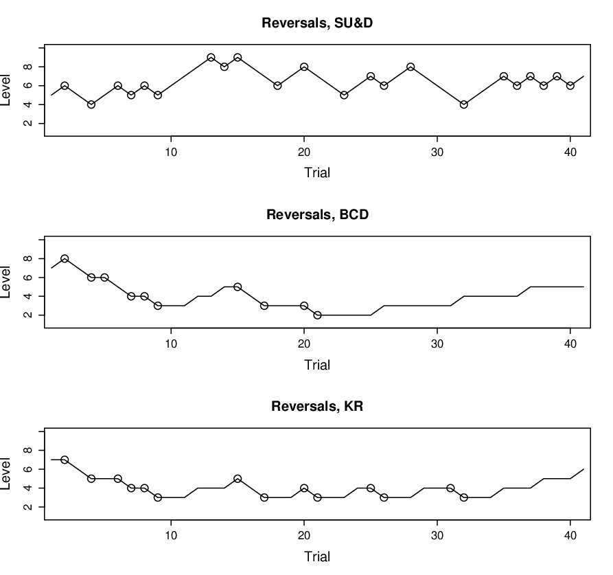
This is where the notion of “reversal” comes into play. A reversal is a point in the experiment, where the response is different from the previous, i.e. a reversal at means that . For SU&D, reversals are where the treatment chain reverses direction, hence the name. For the U&D variants described above, that is not necessarily the case; however, the term “reversal” has been used for them under the same definition. Brownlee et al. (1953) were the first to suggest discarding all data up to the first reversal, using ‘common sense’ arguments. Wetherill (1963) suggested “down-shifting” at the first reversal, an idea that has recurred in different forms since then. Interestingly, “down-shift” schemes triggered by the first reversal have been prominent in recent attempts to integrate U&D into model-based Phase I designs (Storer, 1989; Storer, 2001; Potter, 2002). In some fields, reversals are also used as a stopping rule, with the experiment length specified in reversals instead of trials (Garcìa-Perez, 1998; Paul and Fisher, 2001).
The benefit of using the first reversal as a down-shift point has not been verified theoretically. Numerically, both Garcìa-Perez (1998) and this author (Oron, 2005) have concluded that down-shift schemes are not a guarantee for performance improvement. More generally, the theoretical properties of reversals have not been studied since Wetherill (1963).
2.1.5 Other Up-and-Down Descendants
Beyond the straightforward modifications described above, U&D has spawned a wide variety of related designs over the years. Wetherill (1963) was the first to lay out a catalogue of such designs. In psychophysics, a popular family of related designs mandates a different step size for ‘up’ and ‘down’ transitions (Garcìa-Perez, 1998; Garcìa-Perez and Alcalà-Quintana, 2005). If the step size ratio is irrational, the range of levels becomes continuous. Another related family is that of Polyà urn schemes (Rosenberger and Grill, 1997). Here the transition probabilities vary as a function of prior responses, according to a predefined algorithm. That family has been less extensively studied.
Given the significant gaps in knowledge about the simpler Markov-chain U&D designs, these non-Markovian U&D descendants are outside the scope of my dissertation.
2.2 Theoretical Study
2.2.1 Conceptual Prelude
The U&D design family achieves a remarkable feat: it converts censored, binary-response (and therefore indirect) threshold sampling – a rather unfriendly turf for percentile estimation – back into direct sampling from a quantitative distribution on the threshold/treatment scale. This distribution is , the stationary distribution of treatments. Even better, appears to be centered near . These properties are even more remarkable, considering that the method was developed not from a deep understanding of Markov chains, but rather using ad-hoc intuitive innovation.
The properties of suggest a very natural estimator for : the empirical mean. How well such an estimator performs, depends on how quickly we can assume to be sampling from , and on how well is centered around target. These will be some of the topics discussed below. But first, for lack of a standard reference, some foundational definitions of basic concepts are needed – as well as a careful study of KR’s properties.
Notational comment: from here on, I will use as a shorthand for .
2.2.2 Definition of Target and Mode
The concept of U&D target has been somewhat ill-defined in research. Most (Gezmu and Flournoy, 2006, e.g.) are content with a general intuitive notion, similar to that of the method’s originators. Giovagnoli and Pintacuda (1998) attempted a more rigorous approach; however, they end up defining target only for a narrow (and somewhat contrived) subset of U&D designs, which does not cover KR or GU&D. I have found the following definition useful, broad and rigorous, and in the spirit of the original idea:
Definition 2
Consider an ‘Up-and-Down’ design with a stationary distribution , and with (marginal) stationary ‘up’ transition probabilities continuous monotone decreasing in , and ‘down’ probabilities continuous monotone increasing in , respectively. The design’s target is defined as the value such that
| (2.6) |
Ivanova et al. (2007), in a concurrent paper, have suggested a similar definition for GU&D’s target. In words, the target is the value from which marginal stationary ‘up’ and ‘down’ probabilities would be equal, had a design level been placed exactly there. It is straightforward to see that this definition does recover SU&D’s and BCD’s targets as the median and , respectively. It is also equivalent to the definition appearing in Giovagnoli and Pintacuda (1998) on the subset discussed there. The reason for including the terms “stationary” and “marginal” in the definition will become clear below.
This is also a good occasion for defining the notion of a single mode. The definition is followed by a useful result about the mode’s location w.r.t .
Definition 3
Let be an U&D (marginal) stationary distribution. Then will be said to have a single mode, if the set of indices and has either a single member or two members with adjacent indices .
Lemma 1
If a U&D (marginal) stationary distribution’s profile is continuous and strictly monotone decreasing in , then
(i) The distribution has a single mode.
(ii) If there exist two adjacent levels , such that , then the mode is either at or at .
Proof 2.2.1.
(i) If or , then the mode is obviously on the lower or upper boundary, respectively. In the remaining (and more interesting) case, there has to be some such that , with equality holding for at most one of the relationships. By the definitions of and of the mode, the mode is at , possibly with either or (but not both). Due to monotonicity, this mode is unique.
(ii) Note that the following inequality always holds for any (except on the lower boundary – a case that can be omitted here w.l.o.g.), under the specified conditions:
| (2.7) |
Therefore, for all , and for all , . Recalling (i), this means that the mode has to maintain . Together with ’s monotonicity, this forces the mode to be within of .∎
2.2.3 Basic Properties of ‘K-in-a-row’
We now return to the ‘k-in-a-row’ design (KR). Unlike SU&D, BCD and GU&D, KR does not generate a first-order random walk. A KR run can be described as a -th order random walk with two sets of transition rules, only one of which applies at each trial depending on the string of most recent treatments (Gezmu, 1996):
However, this description does not explicitly acknowledge the counting of ‘no’ responses before an up transition. For this and other purposes, it is more useful to view KR as generating a Markov chain whose treatments are paired with a sequence of internal states . Each internal state can take one of possible values , for a total of states (cf. e.g. Weiss, 1994, Ch.6). Under this internal-state formulation the transition rules become
| (2.8) |
Note that the terms still pertain to transition between physical treatment levels, and not between internal states. A few more notes on the internal-state formulation:
- •
The are uniquely determined by the ; hence, after the experiment is over it suffices to record , and then can be reconstructed.
- •
In the same vein, a subject receiving a given treatment is oblivious to , which has no practical effect upon trial itself.
- •
For this reason and also for comparison purposes, we ultimately focus upon marginal probabilities and distributions, i.e. values summed over all internal states. The marginal stationary frequency of level will be denoted .
Theorem 1.
(i) KR’s marginal stationary distribution profile is given by
| (2.9) |
(ii) Let the stationary marginal ‘up’ probability of a KR design be the weighted average . Then
| (2.10) |
.
(iii) KR’s marginal stationary distribution has a single mode, which is at most 1 spacing unit away from under the conditions specified in Lemma 1 (ii).
Proof 2.2.2.
(i) Taking the internal-state approach, the balance equations between adjacent treatment levels may be written as
| (2.11) |
Now, transitions between internal states of the same treatment level are possible only for single upward increments, each with probability . Therefore, to maintain balance at stationarity, the internal state frequencies must obey - a diminishing geometric sequence. This enables us to calculate relative internal-state frequencies, and specifically the upper state:
| (2.12) |
(ii) This result is immediate from (2.9).
(iii) Differentiating w.r.t to shows that it is monotone decreasing as increases (a more detailed derivation can be found in Appendix A). Since itself is monotone increasing in , and since is monotone increasing in , is monotone decreasing. Therefore, by Lemma 1, there is a single stationary mode at most spacing unit away from target.∎
A somewhat different proof for result (i) appears in Gezmu (1996).
Under stationarity, the frequencies of internal states within each treatment level form a decreasing geometric sequence. This means that the base () internal state is the most common. Intuitively, this is due to the fact that each level transition (whether up or down) resets the internal state to zero. It may be of interest to look at the distribution of these first visits - i.e., the stationary distribution of a KR chain for which each sojourn at a treatment level is collapsed to a single trial corresponding to the base internal state.
Corollary 2.2.3.
Consider a subset of any KR experimental chain, composed only of base-state trials, i.e. . The stationary profile of this subset is
| (2.13) |
That is, a profile identical to that of a GU&D(k,0,1) design with the same .
Proof 2.2.4.
Conceptually, we can explain this surprising identity: after deleting all trials with , one is left with an SU&D-like (or GU&D(k,0,1)-like) chain, in the sense that it never remains at the same level. Now, from a given level’s base state, the probability of the next transition being an ’up’ one is , and the move must be down otherwise - yielding exactly the transition probabilities of GU&D(k,0,1) (see (2.5)). This result will prove rather useful later on.
2.2.4 Location of the Stationary Mode
We have established that for all U&D variants discussed here, the stationary mode is one of the two levels closest to target. It turns out we can do even better.
Theorem 2.
(i) SU&D stationary mode is located at the level whose value is closest to .
(ii) GU&D(k,0,1) stationary mode is located at the level whose value (with defined in (2.5)) is closest to .
(iii) GU&D(k,a,k-a) stationary mode is located at the level whose value is closest to .
Proof 2.2.5.
(i) Let w.l.o.g. Then we can write , with . Now
| (2.14) |
Therefore, if and only if , with equality only if the two are equal. Since the mode is at one of these two levels, our proof is complete.∎
(ii) This part follows immediately from (i) and from the definition of .
(iii) First, note that for the binomial cohort-outcome r.v. defined in the previous section, . Moreover, both sides of the equation are monotone increasing in . Now using the same notation of part (i),
| (2.15) |
Again, if and only if , with equality only if the two are equal.∎
For median-finding U&D, the stationary mode is the closest to target on the response scale. For GU&D(k,0,1), this is true on the transformed scale of . Since is convex in , on the original response scale the transformed midpoint lies closer to , the lower of the two levels. This means that the “attraction basin” of the upper level is larger, and therefore if the target lies midway between levels on the scale, the mode would revert upward to . However, this asymmetry is relatively small: to first order in , the two “attraction basins” are equal in size.
If one wishes to measure closest treatment on the scale, exact results depend upon the form of . However, to first order in , it is straightforward to show that the treatment midpoint is the boundary between the two “attraction basins” for all designs covered by Theorem 2.
The mode location of the two remaining non-median designs is less symmetric.
Theorem 3.
(i) For BCD designs, and using the same terminology as in Theorem 2, the stationary mode would revert to unless is closer to by a factor greater than .
(ii) For KR designs, the stationary mode would revert to if .
| (2.16) |
and vice versa.
Proof 2.2.6.
(i) This follows directly from substituting from (2.2) in the formula for .
(ii) This follows directly from substituting the analogous KR formulae found in the previous subsection.∎
The KR formula is again more complicated; analysis to first order in yields the approximation
| (2.17) |
for the mode to revert to . For this yields approximately , , respectively, for the ratio at the “basin boundary”. The analogous factors for BCD are , , respectively. So both designs tend to create a mode below target more often than above it – a tendency opposite that of GU&D(k,0,1) – but KR’s tendency is quite a bit milder than BCD’s. This explains the numerical observations of Gezmu (1996), who noted that KR is ‘better centered’ on target than same-target BCD (see e.g. Fig. 2.3). As above, on the treatment scale these same ratios can be used as approximations to first order in .
2.2.5 More Stationary Properties
Peakedness of non-median-target designs
Due to limitations related to the unknown location of target relative to the fixed design levels, the notion of ‘peakedness’ is not easily converted to more familiar terminology used to describe dispersion (e.g. precision or variance), but it carries a similar meaning within the U&D context. The more ‘peaked’ a stationary U&D distribution is around its mode, the closer the method is to the ideal design, and percentile estimation precision will generally improve. Here is a rigorous definition of ‘peakedness’, following Giovagnoli and Pintacuda (1998).
Definition 4.
(i) For two ‘Up-and-Down’ designs, ”all other things being equal” will mean that both target the same percentile, the threshold distribution is the same, the treatment levels are the same and the initial conditions are the same.
(ii) (Giovagnoli and Pintacuda, 1998) Let designs and be two U&D designs. Then, all other things being equal, if for while for (i.e., design 1’s stationary distribution profile is steeper), then design and its stationary distribution are called more ‘peaked’.
Thus, for example, to compare KR and BCD we need to examine
| (2.18) |
Theorem 5.
For any , all other things being equal, KR designs are more ‘peaked’ than BCD designs.
Proof 2.2.7.
Proposition 6.
For KR and GU&D(k,0,1) with the same , neither design can be said to be more ‘peaked’ than the other.
Proof 2.2.8.
The ratio analogous to (2.18) is
The inequality results from the concavity of in . GU&D(k,0,1)’s stationary distribution profile is steeper to the left of the peak, while KR’s is steeper to the right of the peak.∎
Fig. 2.3 provides a numerical example of ‘peakedness’. The differences between methods do not appear to be dramatic. On the other hand, if the spacing is too coarse (e.g. on the left) the stationary peak is very broad and the method’s stationary properties offer only a modest improvement over standard, non-sequential treatment-response designs. As the spacing becomes finer (e.g. on the right), a sharp peak forms: under stationarity, all methods allocate of treatments to the two levels closest to target. Thus, finer spacing dramatically reduces the chance for treatments allocated too far from target. In the scenario illustrated in Fig. , with , ( roughly corresponds to the th percentile here) is to depending upon method, while with the analogous probabilities are to . The figure also shows (for ) BCD and KR’s tendency to have the mode below target, and GU&D(k,0,1)’s opposite tendency. Here and , so KR’s “basin boundary” falls just above target on the scale, while BCD’s and GU&D(k,0,1)’s boundaries are at a larger distance above and below target, respectively.

Peakedness of median-target GU&D designs
Another result related to GU&D ‘peakedness’ was numerically observed by Gezmu and Flournoy (2006): for median-targeting GU&D , the stationary distribution appeared more peaked with decreasing . Here is a general proof.
Theorem 7.
For GU&D designs , and all other things being equal, ‘peakedness’ increases with decreasing .
Proof 2.2.9.
Consider design with and design with , such that . Since the transition probabilities are ‘drawn’ from the same binomial model, they can be represented thus: , where . The ‘peakedness’ ratio is then
| (2.19) |
If (meaning that the target is exactly midway between the two levels if distance is measured on the response scale), the ratio is exactly . Focusing on the fraction on the right-hand-side, the ratio in the numerator is decreasing with while the one in the denominator is increasing. Therefore, the ratio would be with both levels below target and vice versa, and thus by definition design is more ‘peaked’. ∎
2.2.6 Convergence Rates
For U&D methods, the term “convergence rate” can be interpreted in a number of ways. In view of theoretical results about the stationary mode, one may be interested in the convergence of the probability that the empirical mode is the stationary mode, or more generally in the convergence of empirical frequencies to their stationary values. On the other hand, in view of the prevalence of averaging-based estimators, there is practical interest in the convergence of the empirical mean to the stationary mean. Fortunately, the three methods discussed here generate simple Markov chains with finite state spaces, and therefore all convergence rate comparisons should yield equivalent results. Here we focus on the empirical mean, which is the simplest, most intuitive, and carries a direct practical significance for most applications.
As Gezmu and Flournoy (2006) note, for finite-state Markov chains the exact treatment distribution after trials can be calculated, given knowledge of initial conditions and of , the design’s transition probability matrix (tpm):
| (2.20) |
where is an initial probability vector over the levels, is the transpose operator and is raised to the -th power. As , , regardless of . Convergence rates can be estimated using the tpm. The tpm’s of the three Markovian methods discussed here are stochastic and irreducible. Hence, the real parts of their eigenvalues are bounded between and , and are usually labeled in decreasing order: . If the tpm is also reversible, that is , then the eigenvalues are all real. In that case, it can be shown that the total variation distance between and converges to zero with a rate (Diaconis and Stroock, 1991)
| (2.21) |
where is a constant and . Thus, the rate of convergence is governed by the second-largest eigenvalue. For finite-state Markov chains, it is straightforward to show that the empirical mean would converge at half the rate of the total variation distance.
Unfortunately, comparing the methods cannot be trivially reduced to an eigenvalue problem: KR tpm’s (listing all internal sub-states as separate states) are irreversible matrices (Gezmu, 1996). On the other hand, all sub-states of the same external KR level actually represent the same experimental treatment. Therefore, a possible fix is to compare convergence by observing KR’s reversible matrix of marginal transition probabilities, using (2.10). This is analogous to assuming that in KR experiments internal-state balance is achieved much faster than external-level balance.
One relationship can be directly proven without resorting to eigenvalues.
Proposition 8.
Consider a KR and a GU&D(k,0,1) design with the same . Then, all other things being equal, the KR design converges faster to its stationary distribution.
Proof 2.2.10.
Recall Corollary 2.2.3 and the discussion following it, and observe the zero-state-only KR subchain. Its transition probabilities are identical to those of GU&D(k,0,1). However, while the latter must carry out a cohort of trials for each transition, the KR subchain may take anywhere from to trials – on the average, less than . Therefore, it would require less trials to achieve the same probabilistic convergence.∎
In order to investigate convergence rates more closely, an “all other things being equal” numerical time-progression was performed, as in (2.20).88 8 Two sets of initial conditions were examined: beginning at (similar to typical Phase I conditions) or at , over a variety of right-skewed, left-skewed and symmetric threshold distributions, values of and for BCD, KR and GU&D (k,0,1); a second comparison was performed between BCD and GU&D (3,0,2). Table 2.1 shows a subset of the data. The adjectives ‘tight’ and ‘disperse’ for the logistic and log-normal scenarios indicate smaller or larger scale parameters, respectively. Convergence rates were estimated via an exponential fit on the difference between the mean at time and the stationary mean. All calculations – here and in the rest of the dissertation – were performed in R (R Development Core Team, 2005). A summary of results for convergence ‘upwards’ from and some targets appears in Table 2.1 (’downward’ convergence was faster in most scenarios, but the overall pattern was not substantially different; data omitted here). Shown are the number of trials needed for the ensemble mean of the ’s to converge of the way from to the stationary mean. These numbers can be seen as a practical cutoff, beyond which the treatment chain is ‘as good as’ a sample from , at least for averaging purposes (one reason for choosing is because halving the numbers on Table 2.1 conveniently yields the number of trials needed to converge a more lenient of the way).
| “Trials to 99% Convergence” | |||||||||
|---|---|---|---|---|---|---|---|---|---|
| Distribution | Weibull (Shape Parameter) | Logistic | Log-Normal | ||||||
| 1 (Exp.) | 1.5 | 3.5 | 5 | ‘Tight’ | ‘Disperse’ | ‘Tight’ | ‘Disperse’ | ||
| SU&D | 12 | 9 | 6 | 10 | 7 | 9 | 6 | 9 | |
| BCD, | 19 | 17 | 15 | 17 | 14 | 17 | 13 | 16 | |
| KR, | 17 | 14 | 10 | 10 | 10 | 14 | 8 | 13 | |
| GU&D (2,0,1) | 20 | 16 | 12 | 10 | 12 | 16 | 12 | 16 | |
| BCD, | 18 | 15 | 12 | 12 | 12 | 15 | 10 | 14 | |
| GU&D (3,0,2) | 36 | 27 | 15 | 15 | 15 | 24 | 15 | 24 | |
| SU&D | 34 | 26 | 14 | 12 | 13 | 22 | 14 | 26 | |
| BCD, | 44 | 38 | 30 | 31 | 28 | 39 | 23 | 33 | |
| KR, | 39 | 32 | 21 | 21 | 20 | 32 | 17 | 27 | |
| GU&D (2,0,1) | 46 | 36 | 24 | 22 | 22 | 36 | 20 | 32 | |
| BCD, | 44 | 35 | 24 | 23 | 22 | 34 | 19 | 31 | |
| GU&D (3,0,2) | 81 | 57 | 33 | 30 | 33 | 54 | 27 | 51 | |
Some observations from Table 2.1:
- 1.
SU&D converges faster than any non-median method examined. This is intuitively expected, since SU&D requires a only single trial before transition in either direction.
- 2.
For a given target response rate , convergence rates are most strongly affected by a combination of distribution properties and spacing - specifically, by the difference in values between adjacent levels around target. For example, the “shallowest” CDF (exponential thresholds and ) causes the slowest convergence, and vice versa.
- 3.
Among the three non-median methods, KR is solidly ahead, while BCD is slowest. Based on these and other numerical runs not shown here, one could expect BCD to take around more trials than same-target KR to reach the same degree of convergence. The performance gap increases with .
- 4.
The number of trials to 99% convergence can be quite substantial when compared with the design limitations of applications such as Phase I clinical trials. Moreover, the Markovian method most closely resembling the ‘3+3’ design (GU&D(3,0,2)) converges very slowly - even slower than BCD. It takes GU&D(3,0,2) more trials than KR () to achieve the same degree of convergence, even though the former’s target is closer to the median. Furthermore, recall that these are ensemble averages and not single-run statistics.
Table 2.1’s convergence rate estimates are in rough agreement with eigenvalue predictions for BCD and GU&D (data not shown). KR rates show an agreement with the ‘marginalized’ tpm eigenvalue, indicating that indeed it is the between-level convergence that is rate-limiting.
Note that in agreement with Proposition 8, KR converges faster than GU&D(k,0,1). Furthermore, same-targeted BCD is the slowest-converging. This has been observed universally, over a much wider range of scenarios than is reported here. I have yet to find a rigorous proof why. Can a heuristic explanation be found?
The KR-BCD convergence gap recalls the observation by Gezmu and Flournoy (2006) that for median-targeting GU&D with fixed , convergence speeds up with increasing . In both cases, the (marginal) of the faster method are always as large or larger than those of the slower method – and in such a way that the difference is also larger. This means that both the “probability flux” in each direction, and the net flux in direction of target, are larger for the faster method. This is formalized in the conjecture below.
Conjecture 9.
Consider two U&D designs: design 1 with and design 2 with , and all other things being equal. If for all levels, and when are both below or above target, then design 1 converges faster.
Note the similarity to and difference from the ‘peakedness’ definition, Definition 4. Here and there we compare up and down probabilities between adjacent levels. However, ‘peakedness’ is related to the probability ratio, while the convergence conjecture is related to the probability difference (or ‘flux’). In the median-targeting GU&D case, increasing increases the difference while making the ratio smaller; therefore for this design family one faces a tradeoff between fast convergence and sharp stationary distribution. On the other hand, KR maintains both a greater ratio and a larger difference between up and down probabilities, compared with BCD – so it has a performance edge on both aspects.
2.2.7 Bias of Early Reversals
First Reversal
From this chapter’s theoretical analysis, it is now clear that the number of trials to the first reversal is a random variable. Of practical interest is the location of first reversal, denoted , conditional upon starting point . Those who use the first reversal as a cutoff or transition point, implicitly assume that this location is close to target. Let us examine this for GU&D(k,0,1) and KR. For both of them, assuming a start from the lowest level , the distribution will be
| (2.22) |
This distribution is reminiscent of a generalized geometric r.v., with the reversal defined as ‘success’, and with monotonically decreasing ‘failure’ (i.e., passage) probabilities at each trial. If is sufficiently small w.r.t. the slope of , then in the vicinity of the ‘up’ passage probability is approximately . This means that conditional upon reaching , the level immediately below , before the first reversal, the expected additional number of levels traversed is less than - landing us very close to target. However, the expected location of is a weighted average of this and of the expectation conditional upon not reaching :
| (2.23) |
Therefore, under typical design scenarios, if , should be expected to be well below target. Now, suppose , with . Then (2.23) still holds, but now the second term includes the possibility that the chain’s first move would be downward. So again, if is or more levels below target, should also be below target. The same conclusions hold for BCD since eventual transition probability without a reversal is also on target, and is monotone decreasing with increasing . On the other hand, if is close to target, the first reversal will be approximately ‘right on’.
If the experiment begins at the top level , for SU&D the outcome will be similar to that when starting from bottom. For the non-median methods, downward transition probabilities will become at the median - long before reaching target. Therefore, if is at or above the median, the upward bias of should be even greater than the downward bias when starting below target.
This asymmetry suggests that perhaps the interpretation of reversal for non-median-target designs may be wrong. Perhaps, instead of “a point where a change in response is observed” we should define reversal as a point where a change in chain direction is observed, i.e. a move up when the last move was down (ignoring trials that mandate no change). For SU&D the two definitions are equivalent. It is easy to see that for non-median-target designs the second definition causes a symmetry in behavior, as far as first reversal bias is concerned. However, a closer look reveals that direction changes are more likely than reversals to occur far from target (to either side; more about this on Section 3.2). All in all, the potential benefit from this changed definition is not clear, and is outweighed by the added complication. Hence it is more useful to understand the properties of reversals as they are currently defined, and plan our design accordingly.
To sum it up, the location of is in general biased towards , and is not guaranteed to be close to target unless itself is close.
Subsequent Reversals
So we have just learned that unless is very close to target, the point of first reversal is likely to be on the same side of target as (though closer on the average). Since is between and , the second reversal is an even worse choice for cutoff or transition. However, the expected net movement away from target between first and second reversals, is obviously smaller than the expected gain between starting point and first reversal (since probabilities for moving away from target are smaller than for moving towards it). This makes the third reversal an interesting cutoff-point candidate. The next potential candidate is naturally the fifth reversal. Choosing a cutoff point beyond the fifth reversal may be too late for many sample-size restricted applications.
Glossary for Chapters 1-2
Glossary is alphabetically ordered, starting with acronyms, then mathematical symbols (Roman letters first, Greek following). There are additional glossaries for Ch. 3 and Ch.4-5, but this one is the most extensive.
Note: in order to keep the glossary manageable and informative, I chose to omit some symbols which make a one-time appearance somewhere in the text, if they have no general significance.
- BCD:
The Biased-Coin Up-and-Down design developed by Durham et al. (1995).
- GU&D:
The Group Up-and-Down design first developed by Tsutakawa (1967b).
- KR:
The “k-in-a-row” Up-and-Down design, first developed by Wetherill et al. (1966); Markov-chain properties first described properly by Gezmu (1996). The name KR is taken from Ivanova et al. (2003); I use it because it better distinguishes KR from other U&D variants.
- SU&D:
The original median-targeting Up-and-Down design described by Dixon and Mood (1948).
- U&D:
Up-and-Down. In this thesis, I use the name U&D to refer to the family of designs that generate Markov chains whose stationary distribution is centered on the target percentile. Includes (though not limited to) BCD, GU&D, KR and SU&D.
- :
The lower and upper transition criteria parameters in group U&D designs. If ‘yes’ responses are observed in the -sized cohort, a move ‘up’ is mandated, and if are observed a move ‘down’ is mandated.
- :
The CDF of thresholds; throughout the thesis, assumed to be strictly increasing and to have a density.
- :
The threshold density; first derivative of .
- :
The value of at treatment level .
- :
A transformed CDF of thresholds for a certain family of GU&D designs (see text for details). The concept of “transformed CDF” was first offered in this context by Wetherill et al. (1966), where it was used erroneously for KR-type designs.
- :
Used for indexing trials and responses.
- :
The number of consecutive ‘yes’ (’no’) responses needed for a move ‘up’ (’down’) in below-(above-)median KR designs; the cohort size in group U&D designs.
- :
Treatment level, indexed .
- :
The number of treatment levels (if finite)
- :
Ensemble size (i.e., number of individual runs) used in simulations.
- :
Sample size of a single experiment.
- :
The target response rate.
- :
The transition probability matrix (tpm) of an U&D design.
- (indexed):
The U&D ‘up’, ‘down’ and ‘stay the same’ probabilities, respectively, at level .
- :
The -th quantile (or -th percentile) of . , with specifically the target response rate, is the experiment’s target.
- :
Index denoting the location (between and ) of the -th reversal point.
- :
The spacing between adjacent treatment levels (assuming levels are evenly spaced).
- :
The response-threshold r.v. Viewing a binary-response experiment as thresholds being triggered by the treatments, underlies the entire statistical approach to the percentile-finding problem. Individual thresholds are then assumed to come from some (generally unknown) distribution with a density .
- :
Actual values that takes.
- :
Used for indexing treatment levels.
- :
The internal state at trial in a KR experiment, so that the current state of the experiment is fully described by the pair . can take integer values from to .
- (generic):
The treatment as an independent variable (in the algebraic sense).
- (indexed):
The treatment value at trial of an U&D design.
- (indexed):
The binary response at trial .
- :
The cohort response variable in group U&D experiments. It is binomial rather than binary.
- :
The BCD “biased-coin” parameter. It is equal to , but is retained here for terminological compatibility with other publications.
- :
The “stationary profile”: the ratio between adjacent stationary frequencies, .
- :
The “stationary profile” as an algebraic function of the independent variable .
- :
The -th eigenvalue of the tpm , arranged in decreasing order.
- :
The stationary and/or limiting distribution of treatment allocations.
- :
The probability distribution of treatments (across levels) at trial .
- :
Used for indexing internal states in KR designs.
Chapter 3 Nonparametric Up-and-Down Estimation
3.1 Existing Estimators and Current Knowledge
Nearly all U&D target estimators can be divided into two groups: averaging estimators, making direct use of the treatment chain only; and response-based estimators, making use of both treatments and responses. This chapter will discuss each type separately, in alternating order. Only the numerical study (Section 3.4) will compare them to each other. As the chapter’s title indicates, the focus is solely on nonparametric estimators.
3.1.1 Averaging Estimators
History and Basic Description
Early U&D estimators were modified averages of the treatment chain, with the modification coefficients based on normal theory (Dixon and Mood, 1948; Brownlee et al., 1953; Dixon, 1965). Tsutakawa (1967b) studied the properties of an average of all trials beginning with , and found a nonparametric expression for its variance (see further below). However, the U&D estimator of choice in most fields is reversal averaging, introduced by Wetherill and aptly named (Wetherill et al., 1966).11 1 Interestingly, Wetherill’s reasoning for favoring reversals over all treatments was less theoretical than numerical: this estimator performed somewhat better in simulation. The estimator is a somewhat modified arithmetic average of at reversal points (reversals were defined in Section 2.1):
| (3.1) |
where is the number of reversals. A straightforward reversal average is known as , introduced by Choi (1971). Estimators belonging to the or type (i.e., some average of treatments at reversals only, beginning from a certain cutoff point) appear to be the most commonly used U&D estimators in median-finding applications across most relevant fields, and in psychophysics experiments using KR. From here on I will refer to this estimator family as .22 2 It should be noted that according to Pace and Stylianou (2007)’s recent meta-analysis of 16 U&D anesthesiology experiments published in 2000-2006, half the studies still used Dixon and Mood (1948)’s original estimator, with only second in popularity. As Choi (1971) pointed out, for SU&D is identical to the simpler when is even, and differs from it by when is odd. For KR and other non-median methods, this is not the case, but the two are still very closely related.
Considering its prevalent use, has received very scant theoretical attention in its years of existence. In the 1980’s, Kershaw (1985); Kershaw (1987) looked at stationary properties, especially variance, and concluded that is in fact inferior to Dixon and Mood’s original estimator. Kershaw’s conclusions were largely ignored, and continues to be the most popular U&D estimator. More recently, Paul and Fisher (2001) conducted a numerical study of in the context of anesthesiology experiments. They concluded that or more reversals are needed for reliable estimation, contrary to a prevalent practice by some groups in that field that use only .
Dixon (1965) claimed without proof, that SU&D’s empirical mean (apparently under stationarity) is unbiased if has a symmetric density. Garcìa-Perez (1998) simulated stationary SU&D and KR runs (using the last reversals from runs having reversals each), finding that for KR is biased towards the median (a bias that is of course zero for SU&D).
Finally, the empirical mode can be seen as related to averaging estimators. Markov-chain studies (Durham et al., 1995; Giovagnoli and Pintacuda, 1998) prove that the empirical mode converges to the stationary mode, which is guaranteed to be one of the levels closest to target. However, we saw in Section 2.2 that the stationary mode may end up being only the second-closest level to target, especially for BCD and KR designs. Additionally, the mode is restricted to be at a treatment level, while averages can vary on a finer scale and hence are more precise. It is therefore not surprising that numerical studies find this estimator performs poorly (Durham et al., 1997; Stylianou and Flournoy, 2002; Oron, 2005). The empirical mode will not be discussed further.
Mitigating The Starting-Point Effect
Perhaps the most obvious problem with averaging estimators is starting-point bias. The first treatment is completely arbitrary (even if determined with good judgment). Then, somewhere during the experiment, the chain begins meandering around target. But at what point does the chain become “good enough” to include in an averaging estimator? Since during U&D’s formative years it was not understood to generate a Markov chain, solution approaches had developed gradually and intuitively. Brownlee et al. (1953) recommended discarding (they were also the first to note that is uniquely determined by the experiment, and incorporated it into the estimate instead). Dixon (1965) and then Wetherill et al. (1966) recommended starting from the first reversal. Much more recently, Garcìa-Perez (1998), based on extensive KR simulations, recommended starting from the 2nd or 3rd reversal. In practice, most researchers use all reversals for , but some discard the first .33 3 Garcìa-Perez (1998) tabulates a meta-analysis of KR vision research experiments published in the mid-1990’s. The vast majority of the 82 studies used some form of reversal averaging. Out of 60 reversal-averaging studies for which information was available about initial-sequence removal, 32 removed no reversals, 14 removed the first 1-2 reversals, 12 removed 3 or more reversals, and 2 used some other criterion.
In the previous chapter, we have seen that in general the first reversal point is quite likely to occur while the starting-point bias is still substantial. We will revisit this issue, and novel ways to tackle it, later on.
Mitigating The Boundary Effect
When the treatment set is finite and lies too close to a design boundary, averaging estimators will display a strong bias away from that boundary (this point will be explained in more detail in the next section). Garcìa-Perez (1998) offers an interesting fix for this problem, dubbed “layover boundary conditions”: one continues the experimental bookkeeping (for averaging purposes) as if there was no boundary. However, in case levels beyond the boundary are indicated, the boundary treatment is administered. For example, if , and the transition rules indicate an upward move, the next treatment will be recorded as but administered at . Afterwards, the chain will have to move back down “through” before reaching .
Layover boundary conditions are equivalent to assuming that remains constant outside the design boundaries. The treatment chain becomes infinite-state, but since transition probabilities beyond the true boundaries are equal to those at the boundaries, the stationary frequencies of the ‘phantom’ levels constitute a diminishing geometric sequence, and so still exists. This issue, too, will be inspected more closely later on.
3.1.2 Response Based Estimation: Isotonic Regression
Response-based averages use , the empirical binomial point estimates of at design points, created by tabulating the responses:
| (3.2) |
Probit and logit regression are occasionally enocountered in U&D applications (Storer, 1993; Camorcia et al., 2004). Being parametric, they exhibit the usual pros and cons, with their quality depending mostly on whether the model family provides a fair approximation of . Parametric U&D estimators will not be discussed here.
A nonparametric response-based estimator - isotonic regression, which is in fact the NPMLE - was recently introduced to U&D in the Phase I context, and has been recommended by the NIH (Stylianou and Flournoy, 2002; Stylianou et al., 2003; NIEHS, 2001). This innovation has yet to reach all other fields using U&D; and perhaps for the better, since it was not directly compared with which it aims to replace. This comparison appears further below in the numerical study.
Isotonic regression (IR) is a well-known nonparametric solution for a variety of statistical problems (Barlow et al., 1972; Robertson et al., 1988). IR can be produced via a couple of lengthy-named algorithms (pool-adjacent-violators-algorithm, or PAVA; least-convex-minorant), but in fixed treatment-response design context it boils down to a set of binomial point estimates: the original point estimate wherever there is no monotonicity violation, and an estimate pooled from the responses at adjacent levels in case of a violation. The procedure is described in Algorithm 1 below.
PAVA replaces any subsequence of it deems “violating” by a sequence that is a repetition of a single value (which in the case of treatment-responses designs is simply the overall proportion of ‘yes’ responses over the subsequence). This means that the IR estimate of is constant over any interval of values covered by a violating subsequence. In intervals between non-violating design points, IR provides no unique estimate. Since in order to find the percentile one has to perform an inverse estimation, we need a (forward) estimate of over the entire range. In treatment-response applications this problem is commonly solved by linear interpolation (Dilleen et al., 2003; Stylianou and Flournoy, 2002, e.g.).44 4 apparently, in some fields people still believe that a straight line is the simplest way to connect two points. So statisticians have their work cut out for them :).
| Treatment | Raw Input | IR Output | Raw Input | IR Output | ||||||||
| Yes | No | Yes | No | Yes | No | Yes | No | |||||
| (Simulation Run 14) | (Simulation Run 9) | |||||||||||

The operation of IR on treatment-response data is illustrated in Table 3.1 and Fig. 3.1. Shown are two simulated runs, in each of which there was a single violating pair. Assuming the target is , in Run 14 (LHS of both table and figure) exactly; however, . Therefore, technically we cannot determine a unique estimate via linear interpolation between values; and conceptually, neither nor can be fully “trusted” without more information. IR resolves this by pooling the data from points together; the final estimate for is to the right of point . In Run 9 (RHS) we see an (extreme, but possible whenever is rational) example for IR’s limitations: the flat stretch produced by the process lies exactly at , and therefore IR does not provide a unique inverse estimate without some additional convention (taking the highest/lowest/midpoint of possible estimates, etc.). These two numerical examples will be revisited in Section 3.3.
Why is IR the NPMLE for our application? Let us examine U&D’s nonparametric likelihood; it can be written as
| (3.3) |
where the were defined above in (3.2). The derivation uses the following properties:
- •
Given each treatment , the corresponding response depends on no other treatment or response, since the underlying threshold sampling is i.i.d.;
- •
Given all previous treatments and responses, can be found either deterministically, or (for BCD) using a separate, independent random draw which is unrelated to .
Hence, the “const” appearing in the equation is either a product of functions of the biased-coin parameter (for BCD), or simply (for all other designs).
The form of (3.3) is identical to a product of binomial likelihoods, except for having different constant coefficients (the binomial likelihood has combinatorial coefficients). A product of binomials is the nonparametric likelihood of a standard non-sequential treatment-response experiment. Note that the nonparametric approach yields a likelihood that can be interpreted parametrically, as having parameters representing the true values .
Now, since the log-likelihood takes the form
| (3.4) |
the unconstrained NPMLE is of course just . Under monotonicity constraints, proceeding recursively from the first monotonicity-violating pair of values and treating one pair at a time, it can be easily shown that the constrained NPMLE is identical to PAVA’s output. More detailed derivations appear in standard references (Barlow et al., 1972; Robertson et al., 1988).
The “flat” intervals produced by PAVA in case of a monotonicity violation in appear to hurt estimation performance, both forward and inverse. I will inspect this suspicion more closely in the next section.
3.1.3 Interval Estimation
Nonparametric U&D interval estimation has been even more seldom studied than point estimation. However, interest in this topic as well has been picking up recently.
SD-Based Approaches
Dixon and Mood (1948)’s original averaging estimator came with a variance estimator based on normal theory. Pollak et al. (2006), using numerical simulations of material-fatigue SU&D testing, show that this variance estimator performs very poorly, and is strongly dependent upon the spacing . They suggest a 3-parameter empirical correction function fitted to their data.
In anesthesiology, some researchers using SU&D with report confidence intervals. In calculating standard errors, they seem to count each pair of reversals as a single independent observation, and assume asymptotic normality of the average, hence the method’s name: “independent paired reversals” (Capogna et al., 2001; Camorcia et al., 2004).55 5 To be honest, up till now (summer 2007) I have yet to find a full documentation, nor a reference for “independent paired reversals”. The observation reported here is based on “reverse engineering” of reported estimates in anesthesiology articles using the raw data, and I am not sure that it is correct.
Tsutakawa (1967b) pursued a Markov-chain based approach. He noted that a stationary Markov chain can be split into subchains, identified by successive hitting times at a given state - i.e., the points at which the treatment chain visits the state. The lengths of these subchains, , are i.i.d. random variables, as is any algebraic functional on the treatments, calculated separately per subchain. Tsutakawa (1967b) then goes on, basing his calculations on Chung (1960, Ch. 1), and claims that
| (3.5) |
as . Therefore, he proposes the LHS of (3.5) as an estimator of the variance for the empirical-mean estimator. However, from data tables in that article, as well as my own numerical trials, it seems that the LHS approaches the limit from below, and therefore the resulting CI’s are too optimistic.
Another approach to averaging-estimator confidence intervals was presented by Choi (1990). Starting from first principles, the variance of the average of r.v.’s is
| (3.6) |
Now, being part of a Markov chain, values at reversals are clearly dependent. Assuming that they are identically distributed and that dependence follows an AR(1) autoregressive form, Choi (1990) obtains formulae for the s.e. of as a function of the threshold s.d. and the autocorrelation coefficient . Additionally assuming normally-distributed thresholds, CI’s can be calculated. Choi (1990) found them to be overly optimistic, but better than Dixon and Mood’s original CI’s.
Bootstrap Approaches
Recently, use of the bootstrap for U&D CI’s was explored – both for parametric estimation (Chao and Fuh, 2001) and for for isotonic regression (Stylianou et al., 2003). The bootstrap approach for U&D is to simulate chains of length , with transition probabilities determined via some estimate of (IR or a parametric regression). In both cases, however, the bootstrap was used not for CI’s around , but for CI’s around the forward estimate of at the closest design level. Chao and Fuh (2001) used the ordinary bootstrap and bootstrap-, while Stylianou et al. (2003) used the bias-corrected bootstrap (see Davison and Hinkley, 1995, Ch. 5). Pollak et al. (2006) explored using the bootstrap combined with their empirical fix to Dixon and Mood (1948)’s formula, and reported good results.
Use of Current-Status Theory
Recalling that U&D is a special case of current-status data, there is a wealth of theoretically-derived interval estimation knowledge in that field (Banerjee and Wellner, 2005). However, U&D appears to be too special a case: under the typical current-status assumptions, treatments are random with a continuous CDF. This leads to an rate of convergence everywhere for the NPMLE. U&D, though its treatments are random, is more akin to standard treatment-response designs in that treatments are limited to a discrete finite grid – while the continuity of treatments is a key assumption in most current-status CI discussions. As a result, the point estimates converge with an rate, and the linearly-interpolated IR used in U&D converges at the same rate - but not to , but rather to - a linear interpolation of between the design points. Therefore, it appears that current-status CI theory is not applicable to U&D interval estimation.
3.2 Theoretical Study
3.2.1 Conceptual Prelude
We have at our disposal two nonparametric approaches to U&D estimation. The response-based one is generic to any binary-outcome design. It does not make direct use of the properties of , but benefits indirectly from having more precise estimates in the vicinity of . Averaging estimators, on the other hand, are intimately related to the peculiar properties of U&D sampling.
Considering the stationary properties already discussed here, one can say that some sort of empirical treatment mean is the “natural estimator” for U&D designs. I put forward this rather strong statement, in order to re-emphasize the conversion trick that underpins averaging estimation. U&D converts censored sampling back into direct sampling – which, as suggested in Section 1.2.1, would be far more desirable than indirect, binary censored sampling.
However, to utilize the potential of averaging estimators, we need to better understand the properties of and of random-walk sampling from it. Unfortunately, since the averaging estimators currently in use were developed without the Markovian perspective, they do not utilize the full estimation potential. In particular, choosing to average reversal points means that we are not sampling from itself, but from its “sibling”: the stationary distribution of reversals. Much of this section will be devoted to untangling the peculiar properties of such sampling, and to suggesting other approaches.
Meanwhile, even though isotonic regression is not “natural” in the sense discussed above, this also means that it suffers less from U&D’s peculiarities and limitations, such as starting-point bias or boundary effects. Therefore we expect it to be more robust, and will look at its properties more carefully later on.
3.2.2 Estimation Properties of Treatment Means
Bias of the Stationary Mean
We have already seen that for median-targeting designs and for GU&D(k,0,1), the stationary mode is on the closest treatment to target on the response scale - which is also the closest on the threshold or treatment scale (to first order in ). BCD and KR tend to shift the mode somewhat to the left of target. One could expect, therefore, that with the former variants the stationary mean would show little or no bias w.r.t. , while with the latter there would be a downward bias, or more generally, a bias away from the median.
More insight into stationary biases can be gained via a telescopic-series analysis. First, note that in the limit of infinitely fine design (), the stationary biases of BCD and KR, too, should vanish. Therefore, we may expect the bias magnitude to be related to . In the subsequent discussion, we assume that there are no design boundaries (i.e., the treatment set is potentially infinite) that is twice continuously differentiable in , and also – for convenience – that falls exactly on (letting land midway between design levels is nearly as convenient).66 6 Numerical runs (data not shown) seem to indicate that biases related to design offset w.r.t to target are much smaller than the spacing-related bias discussed here. One can then express the stationary mean as a telescopic series around target:
| (3.7) | |||||
Since the stationary frequencies diminish in a faster-than-geometric rate away from , the sum is typically dominated by the first summand pairs. The pairs are composed of opposite-sign terms, which may nearly cancel out. We now carry out a detailed calculation of the first pair for SU&D.
First, note that if has a symmetric density, for SU&D the terms in each pair will cancel each other exactly. So apart from design-offset biases, SU&D averaging estimation is indeed unbiased as claimed by Dixon (1965). For asymmetric distributions, we would need standard Taylor expansions around target:
| (3.8) | |||||
where is the threshold density and its derivative. Substituting this and setting , the first summand pair then becomes
| (3.9) | |||||
The first-order terms cancel out, and we are left with a bias that is second-order in with a sign opposite that of (for unimodal or monotone-decreasing threshold densities, this means a bias in the direction of ’s skew). It is quite straightforward to show that all summand pairs in (3.7) for SU&D give similar negative second-order terms when thus expanded. Therefore, it appears that SU&D’s stationary mean is a biased estimator of for asymmetric densities. However, this bias can be kept very small under reasonably fine spacing.
The same analysis for BCD yields
| (3.10) | |||||
and for KR
| (3.11) | |||||
In both cases there is a downward (i.e., away from median) first-order bias. BCD’s bias term is larger than same-targeted KR, by a factor of about (the exact ratio as a function of is found by substituting KR’s target (2.4) for ). GU&D(k,0,1) “inherits” the properties of SU&D, meaning that its bias is only second-order and therefore usually smaller than that of the other two methods. For symmetric or upward-skewed threshold distributions (a realistic assumption when dealing with positive thresholds), GU&D(k,0,1)’s bias is positive, i.e., towards the median.
So we have seen that stationary biases are approximately first-order or second-order in the spacing, depending upon the design. All these finds are in line with numerical observations such as Fig. 2.3 and with the theory in Section 2.2. Numerical results indicate that for all four variants, stationary biases are quite moderate except when using very coarse spacing.
3.2.3 Averaging All Treatments or Only Reversals?
The simplest candidate to replace the reversal average is some average of all treatments (possibly starting from a certain cutoff point); let us call this latter estimator . Wetherill et al. (1966)’s simulations showed as having smaller MSE than , and this is why it was chosen. Since then, other simulations (Kershaw, 1985, e.g., ) have shown the opposite. Can we make a more theoretical comparison between the two options?
Reversals as a Filter
Assuming stationarity, the frequency of reversals at each level should also become stationary. However, the stationary distribution of reversals is not necessarily identical to . We can calculate it using and the balance equations:
| (3.12) | |||||
where we implicitly assumed that ‘up’ and ‘down’ transitions occur only after a ‘no’ or a ‘yes’, respectively, and that staying at the same level (if possible) also follows a ‘no’. Conveniently enough, the (relative) stationary reversal frequency at a given level is a linear function of at the same level. This means, that picking only reversals can be viewed as a secondary, linearly filtered sampling from .
For SU&D, (3.12) translates to
| (3.13) |
where the normalizing proportionality factor has been omitted. So the filter is distorting: levels far from the median are over-sampled compared with those near the median, by a factor of up to - which means that the stationary variance of reversals is larger than that of the entire chain. If the threshold density is exactly symmetric, the sampling does not induce a bias to the averaging estimator. But if it is asymmetric, the sampling induces a slight bias in direction of the distribution’s skew – i.e., in the same direction as the stationary-mean bias.
For BCD, is proportional to
| (3.14) |
which reduces to (3.13) under . The sampling coefficient’s minimum point, as a function of , is at
| (3.15) |
The minimum moves to the left of as decreases; it is positioned at zero for . Thus, for most or all of ’s range, sampling probability increases with - meaning that BCD reversal averaging induces a bias towards the median. Here, too, we expect to have larger variance, since the filtering is more aggressive near target.
For KR we get
| (3.16) |
Again, the formula reduces to (3.13) for . KR sampling has the same qualitative properties as BCD (i.e., bias towards the median and a larger stationary variance), albeit milder. The filtered sampling coefficient has a minimum slightly to the left of target.
Note that for BCD and KR, ’s additional bias is in the opposite direction of ’s stationary-mean bias. This leads to the interesting question whether the two cancel out. First-order analysis indicates that the reversal bias may be of comparable magnitude, but is generally smaller than the stationary-mean bias. The exact interplay between the two would depend upon specific distribution and spacing conditions.
Variance Comparison
One way to generically describe the variance of a dependent-sample average is
| (3.17) |
where is an effective sample size, usually smaller than . We have seen that under stationarity, for reversals is larger than for all trials. What about ? This is a measure of the information content in the sample about the distribution of trials (or reversals). But reversals are a subset of the sample used for ; their information content cannot be larger. Therefore, .
Instead of this intuitive and not quite rigorous approach, it is also possible to obtain the same result via a direct and more tedious approach for some of the designs.
Proposition 10.
For SU&D and GU&D(k,0,1) designs, under stationarity .
Proof 3.2.1.
We slice the chain into subchains, each beginning with a reversal and ending right before the next reversal. For each subchain indexed , let be the subchain’s treatment mean. A simple average of is equal to which is known to be equivalent to . Meanwhile, is an average of the ’s, weighted by the subchain length . Which one has smaller variance?
If shorter subchains have a higher probability of being farther away from , the population mean of the ’s (which is equal to ), then definitely , since the latter down-weights them. Now, at a given level , the length of a subchain ending with the next reversal is a generalized geometric r.v. with increasing “success” probabilities (”success” being a reversal). However, the subchain-terminating “success” probabilities are always larger in the direction away from , which (ignoring boundary conditions) is very close to . Therefore, subchains are expected to be shorter, the farther their center is from , and hence .∎
For BCD and KR, this approach encounters some difficulties. Now is not a weighted average of ’s, but somewhat smaller than that average because ascent subchains are “bottom-heavy” (recall that is biased upwards w.r.t ). Subchains still tend to be shorter when they are oriented away from , but because of the upward bias we are not quite sure how close is to . However, since the biases (of w.r.t to and of w.r.t ) are opposite in sign, there is little reason to expect a different relationship between the two variances for BCD and KR.
3.2.4 Isotonic Regression and Bias
As detailed in Section 3.1, whenever isotonic regression (IR) departs from simple linear interpolation, it produces constant intervals. Besides being problematic for inverse estimation of quantiles, since we assumed to be continuous strictly increasing this may generate biases. Specifically, if is as assumed, then any estimator producing a constant interval is either unbiased only at a single point on , or is biased across the entire interval. Common sense suggests that if IR is based on unbiased estimates , then the former case is far more likely. This can in fact be proven in some specific scenarios, such as normal errors with variance inversely proportional to the IR weights.
The proof requires two preparatory lemmas.
Lemma 11.
Assume that at each treatment level we have a raw point estimate , which is normal with mean and variance , and that all point estimates are mutually independent. Then for each sequence of points indexed which are replaced by a single value in the PAV algorithm (hereafter: a violating interval), the pooled IR estimate is independent of the degree of the last violation in the sequence, i.e.
| (3.18) |
where denotes a weighted average of values from through .
Proof 3.2.2.
Let be independent normal r.v.’s with variance
Then , a linear transformation of , , will be normal with variance . Specifically, , with some constant, will have a variance
Therefore, .
Now take a violating interval extending from to , and set . Then
while
The two are independent, and
i.e., an average of the two with weights inversely proportional to variances. By the proof above, this average is independent of the difference , which in our case denotes the degree of last violation in the sequence.∎
Lemma 12.
Under the same assumptions, the weighted average is independent of the event that the points indexed are part of a violating sequence starting at .
Proof 3.2.3.
By induction. Let the event in question be denoted . For , the identity follows directly from Lemma 11.
For , assume , and prove for . Due to the independence of the -s, trivially . Now the event . But by Lemma 11, . Therefore it is also independent of the intersection of these two events and the proof is complete.∎
These two lemmas show that weighted averages such as those produced by the PAV algorithm, are invariant to monotonicity violations (under the specified distributional assumptions). This clears the way to a simple and useful fix to IR’s flat-interval problem.
Theorem 13.
Under the same assumptions as above, for each violating interval from to , PAVA produces an estimate which is biased upward at and downward at from its unconditional expectations , respectively.
Proof 3.2.4.
From Lemma 12,
the weighted average of over the violating design points. By the strict monotonicity of , .∎
So, for these particular distribution assumptions on point estimates, we have “nailed” the IR estimate to be unbiased somewhere within the flat interval. It follows naturally, that percentile (inverse) estimates around the interval must be biased away from the interval to either direction.
Of course, in a treatment-response case the binomial estimates are not normal. However, the scenario covered by Theorem 13 approximates their asymptotic behavior as , especially if the binomial variance factor is changing slowly over the violating interval.
Therefore, it may be useful to see where in the interval, according to that scenario, the IR estimator is unbiased. The answer is quite simple:
Theorem 14.
Under the same assumptions as above, and if is twice continuously differentiable in , then – the PAVA estimate for a violating interval from to – is unbiased to (Taylor) first order in segment length , only at the weighted-average point
| (3.19) |
Proof 3.2.5.
First, from ’s continuity, strict monotonicity and Theorem 13 we know that there is exactly one point at which is the true value of , and that this point is in .
Now can be written as a first-order Taylor expansion from a single reference point :
| (3.20) |
where are points between and . At , the first-order term vanishes, and therefore to first order,
Clearly, this is also the only location in the interval that removes the first-order term.∎
This result will be used in the next section to improve upon IR.
3.3 New Methodologies
3.3.1 Averaging Estimators
Overview
Averaging estimators are not just commonly used in U&D; surprisingly or not, their performance is also pretty hard to beat under the popular SU&D and KR designs. The convergence of Markov chains implies , the stationary mean, with asymptotically normal behavior and without any further parametric assumptions on . Averaging estimators typically have the smallest variance, and more often than not it is the variance term that dominates estimation performance. Averaging estimators’ major drawback, as the previous section indicated, has to do with biases. Here is a summary of potential averaging estimators biases:
- 1.
Bias towards the starting point .
- 2.
Bias away from the closest boundary.
- 3.
Theoretical bias of itself, as exposed in Section 2.2.
- 4.
If a reversal-only average is used, an additional reversal-sampling bias.
Since there are so many biases in potentially different directions, sometimes they neutralize each other to a certain extent. This is why the reversal-only average occasionally outperforms the all-treatment average in numerical simulations. This phenomenon will be observed numerically later on, in Section 3.4.
Items 2 and 3 on this list can be managed by choosing a sufficiently fine spacing (which unfortunately increases the magnitude of item 1) – and by not imposing unnecessary boundaries. Additionally, for KR designs there is a potentially interesting fix to item 3 (stationary bias). Recall from Section 2.2 that KR’s sub-chain of base states (i.e., picking only the first trial of each visit to a treatment level) has an identical stationary distribution to that of GU&D(k,0,1). This means that averaging only over the zero-state sub-chain may help us get rid of KR’s first-order stationary bias.
for general designs, the first item on the list – the starting-point effect – has received the most attention in devising new estimators.
Let be the average of all reversal points from reversal onward; according to Garcìa-Perez (1998), this is the most popular estimator in vision research for KR designs. Our analysis up to now indicates that it should be outperformed by , the corresponding all-treatment average starting from the same reversal point. How should be chosen? This is a classic bias-variance dilemma: the farther out we push the cutoff point, the starting-point bias w.r.t decreases, but the variance increases.
Or perhaps there is another way out? Are reversals a good cutoff choice at all? The previous section showed that under stationarity reversals have a larger variance than a randomly-chosen treatment. This means their expected distance from is larger. Since stationarity is in fact a best-case assumption, it seems that reversals are not a very good choice for cutoff.
A New Adaptive Estimator
Another approach seeks to adaptively identify the length of the initial transition phase. The underlying assumption is that the latter phase of the chain resembles a sample from . If so, the average of the chain’s “tail end” is close to . Meanwhile, the “head” or starting point is arbitrarily fixed to .77 7 A similar situation is encountered in MCMC simulations, where a variety of diagnostics have been developed to determine stationarity. However, MCMC usually involves a very large sample and the ability to run several parallel instances of the same run – privileges not available in the small-sample percentile-finding application. The auto-detect estimator chops off this biased “head”, exactly at the first point in which the chain traverses to the other side of the “tail end” average, compared with the starting point - and then proceeds to average the rest of the chain. Symbolically this estimator can be described as
| (3.21) |
The location of the cutoff point is illustrated in Fig. 3.2
Sometimes, the “tail end” of the chain is an “unlucky draw” containing an excursion far from target; sometimes the entire chain converges more slowly than expected by the experiment’s designers. The auto-detect method would usually identify such cases by placing the transition point relatively late. From an overall performance perspective, using a late auto-detect point is not advisable; the probability that the auto-detect scheme has been fooled by an excursion – conditional upon the value of – increases sharply as approaches . one should therefore set a maximum cutoff , so that if we use as our cutoff. This critical value should definitely be less than . Since it can be argued that the “tail end” needs to be sufficiently longer than the transition phase in order to serve as a reference, values around or seem reasonable. Thus, the auto-detect estimator would be guaranteed to include at least the final two-thirds or three-quarters of the treatment chain.
If one wishes to be even more efficient, this critical value can be compared with the number of trials required to reach the boundaries from (if there are no physical boundaries, visualize “virtual boundaries” around the range in which you realistically expect to fall). Allow for one “switchback” of falling back one level towards before resuming progression. If such boundary-related predictions can be made, then resulting cutoff should be compared with or , and the smaller of the two chosen for For example, if the design is KR with and the boundaries extend levels in each direction, then one needs trials to reach the bottom end including one “switchback”, but trials to reach the top end. Then, if , one can use instead of or , and improve precision.88 8 Clearly, this indicates that for below-median targets should be positioned above the middle of the “effective range”; see Section 3.6.

Conversely, if sample size is flexible, the auto-detect properties can be used to formulate a stopping rule. The experiment should continue until , or until passes a certain value - in both cases promising a sufficient sample size of approximately stationary sampling.
For KR designs, we may also wish to look at – the auto-detect estimator taken only on the zero-state sub-chain. It promises to mitigate both the starting-point and stationary-mean biases simultaneously. This idea has not been explored in detail in this thesis, and may merit further examination.
A Geometrically Weighted Estimator
Instead of trying to locate a cutoff point, we can weight the chain according to convergence theory. In Section 2.2, we saw that
| (3.22) |
where , and is the second-largest eigenvalue of . This justifies the following weighted-average estimate:
| (3.23) |
The weights should be a function that starts near zero, then increases until some transition point where we suspect the bias term becomes small compared to the variance term. The location of this point can be estimated by comparing the standard error of some raw form of with some order-of-magnitude estimate for starting-point bias.
Of course, we do not know and its eigenvalues; however, can be nonparametrically estimated from . provides a nice complement to : the former uses responses to evaluate convergence, while the latter tracks the treatment chain.
Two implementation notes:
- •
The -derived tends to produce optimistic rates, or even no rates (in case there is only one point estimate of falling in ). It is therefore recommended to weight with a prior estimate, say uniform. A Bayesian saturated model, or any other parametric model, are also an option (see Section 4.1). However, there is no reason to ‘overkill’ this estimate of with sophisticated procedures, as it is only used as an aid to determine weights.
- •
Another implementation option is to multiply the decay factor by an ‘acceleration’ factor somewhat greater than . This ensures that the initial run’s weight is indeed smaller than its impact on bias.
At bottom line, has many more “moving parts” than other estimators. Since numerical trials did not indicate an overall performance improvement over the simpler options described above, it will not be discussed again below.
Mitigating the Boundary Effect?
If is less than away from a hard boundary, bias source 2 on the list at the beginning of the section can overwhelm all the rest. The best fix is prevention: not to place a boundary, unless it is physically impossible to continue moving up or down. If treatments are positive, consider placing on a log-transformed scale (as is the default in sensory studies). If they are proportions, consider a log-ratio transform. This is not as cumbersome as it sounds: phrase the treatment levels as parts component B to one part component A, etc. Yet another alternative is to halve the spacing if a boundary seems to play a dominant role; a trigger for halving could be the nd visit to the same boundary, or the first transition decision violates the boundaries. Of course, this would have an impact only if the halving occurs relatively early in the experiment.
Sometimes none of these fixes are available, and we are stuck with a real physical boundary. One existing fix was described in Section 3.1 (Garcìa-Perez, 1998) - continue administering treatments on the boundary, as a proxy for levels beyond it. This fix has the property of over-assigning treatments on the boundary. An alternative, milder fix would be to impute following the experiment by adding virtual treatments at wherever a move ‘up’ was mandated from , and at wherever a move ‘down’ from was mandated (these virtual ‘treatments’ would of course never be administered, only added to the average). the number of treatments added would follow the transition rule (e.g., for KR, virtual treatments would be added each visit to , but only at ). This imputation is equivalent to assuming at the two boundaries. The imputation fix requires no change in experiment planning.
It turns out, again, that neither of these fixes works as well as one might expect. This is because both increase the averaging-estimator variance – an increase which is not necessarily offset by a substantial bias reduction. It seems that, if the chain runs dangerously close to a boundary, one should turn to response-based estimation – which, coincidentally, is our next topic.
3.3.2 Centered Isotonic Regression
Due to the theoretical results on IR bias, culminating in Theorem 14, we may attempt to modify isotonic regression by replacing each constant interval with a single point at the location prescribed by (3.20). To be coherent, the new estimator would perform the same action at intervals that were originally constant as well. Algorithm 2 describes this estimator, dubbed “Centered Isotonic Regression” (CIR).
CIR’s point-estimate output is used to estimate and its quantiles via linear interpolation, including at original design points which have been removed. The following observations may help clarify some more major similarities and differences between PAVA and CIR.
- 1.
CIR produces the same set of unique values (point estimates) as PAVA, but under CIR each value appears only once.
- 2.
Unlike PAVA, CIR requires values as inputs, and modifies them in the same manner as the values. As a result, each unique weighted-average value is assigned to the corresponding weighted-average value.99 9 The point placement prescribed by (3.20) is optimal for the normal-error scenario and seems to work well for the treatment-response case as well. For other scenarios (e.g. a current-status dataset copmosed of 1’s and 0’s only), the formula for the optimal point may be different.
- 3.
CIR identifies ties, too, as violations since they violate strict monotonicity.
- 4.
In the absence of strict monotonicity violations, the two algorithms return the original data.
- 5.
In the presence of strict monotonicity violations, CIR returns a smaller number of points than the input.
Due to the last property, sometimes a boundary point may be removed by CIR. Suppose w.l.o.g. that the original has been removed, and now some is the smallest value for which a CIR estimate exists. Then complementing the CIR output with a constant interval on is equivalent to the IR output on the same interval, and should be regarded as the default. However, in case prior knowledge exists regarding on or outside the boundaries (e.g., ), then it should be incorporated either into CIR’s input (when an appropriate weight can be assigned) or into its output.
Conceptually, the CIR process is analogous to saying: “We have this sequence of point estimates, each perfectly valid on its own, but as a sequence they are suspect due to monotonicity violations. We can pool them together to get a single, more believable estimate; however, this is still a point estimate only, and deserves to be placed at a single point rather than occupy a complete interval.”
Under the normal-error scenario described in Section 3.2 and some additional assumptions, it can be proven that CIR yields a smaller overall estimation MSE than IR, but the calculation is rather cumbersome and uninteresting. In nearly all numerical U&D simulations I have carried out, CIR clearly outperforms IR for quantile estimation (some data will be presented below in Section 3.4). The only case when CIR is not recommended, is when the researchers suspect may resemble a staircase function. In that case, IR’s piecewise-constant output is obviously more appropriate then CIR’s linear smoothing.
| Treatment | Raw Input | CIR Output | Raw Input | CIR Output | ||||||||||
| Yes | No | Yes | No | Yes | No | Yes | No | |||||||
| (Simulation Run 14) | (Simulation Run 9) | |||||||||||||

We now revisit the two data examples from Table 3.1 and Fig. 3.1. Table 3.2 and Fig. 3.3 show the same data, estimated via CIR. Since CIR’s output is strictly monotone (at least between its output point estimates), the quantile estimate for Run 9 (RHS) is now unique. Note that CIR is not a risk-free fix. For example, in Run 9 the CIR estimate of at is , while was only . This is because the new estimate is a weighted average of and – the latter being equal to . From a least-squares perspective (i.e., least-square distance from the original point estimates), CIR is clearly not better than IR. However, with respect to the true the pulling-in of neighboring values to smooth out the estimate in violating intervals (where point estimates are more suspect) seems to pay off.
A Combined Estimator?
Averaging estimators and CIR appear to complement each other: the former typically have smaller variance, and the latter smaller bias. This suggests the simple fix of using their average as a combined estimator. Unfortunately this fix is not successful, because the two estimator types are highly correlated (numerical ensemble correlations are typically around or more). This means that a simple average of CIR and an averaging estimator is likely to have higher variance than the averaging estimator alone. Since estimation error is dominated by the variance term (often over of the MSE is due to variance, see below in Section 3.4), the improvement in bias may be insufficient to offset the variance hit.
Why are averaging estimators and CIR so correlated? Suppose w.l.o.g. that we observe a sequence of above-average thresholds. The response rate at most treatments will be below the population expected values, pushing downward and CIR inverse estimates upward. At the same time, the negative responses will also push the treatment chain itself upward, and with it the averaging estimators.
3.3.3 Interval Estimation
Confidence Intervals for Averaging Estimators
For averaging estimators, our rationale is that we sample from and try to estimate the standard error of the running sample mean. Trials before the cutoff point (be it a reversal or the auto-detect point) are discarded. A simple estimate for the standard error could be of the form
| (3.24) |
where is the sample standard deviation of the sub-chain used for averaging, and is an estimate of the effective sample size – which should be smaller than the sub-chain length, since the sampling is dependent. We can estimate using the approach offered by Choi (1990), again with some convenient simplifications. We assume an AR(1) structure. The variance of an averaging estimator is then
| (3.25) |
| (3.26) |
where is the first-order autocorrelation and is the chain length used for averaging. The approximation in (3.26) is conservative. So our autocorrelation-based sample size estimate is . Since the variance is estimated from the data, we should use a -multiplier with d.f. (or d.f. if ).
A rather different approach follows Tsutakawa (1967b)’s observation that intervals between hitting times are i.i.d. Tsutakawa (1967b) used the complicated formula (3.5) to directly estimate the variance; however, as mentioned earlier this appears to be overly optimistic. Instead, we estimate ’s variance from first principles. Let be the length of hitting-time interval , and let be the treatment mean over the interval (Ideally, we use hitting times at the level closest to target, ). Then each r.v. is i.i.d. across intervals.1010 10 We employ a convention that avoids gaps or overlaps, e.g. that each interval begins with the treatment following the hitting time. Additionally, for KR each sub-state should be viewed as a separate state. Hence, we look only at the first visit to each level (i.e., at visits to only), since those are the most numerous. Now, neglecting possible “leftovers” before the first interval and after the last, averaging estimators can be expressed as
where , as before, is the sample size used for averaging (i.e., from the cutoff point onward). Neglecting the randomness of ,1111 11 For fixed-sample applications this is not a bad assumption. Of course, an approach using hitting-times or reversals (which are related to them) as stopping rules will have to account for ’s variability. we focus on the numerator. For a single interval,
| (3.27) | |||||
where is the stationary variance and is the level used for determining the intervals. Summing over all intervals, normalizing and replacing population parameters by estimates, we obtain the estimate
| (3.28) |
where is the level closest to the point estimate, at which the hitting-times are counted; is the number of hitting-time intervals, is the sample variance of the chain used for averaging, and and are the sample mean-square and variance of interval lengths, respectively. As above, we use a -multiplier with d.f. (or d.f. if ).
Based on bot h theoretical appeal and numerical trials, I chose the second, hitting-time-based S.E. estimate (3.28). In general it is quite conservative. One reason for choosing the more conservative option, is that estimates the stationary mean and not , and therefore the interval will inevitably be somewhat shifted. Sometimes, when the shift is too large (i.e., one of the bias sources mentioned at the top of this section is too dominant), no interval would do the job. This again points to the importance of averaging-estimator bias reduction.
Confidence Intervals for CIR
CIR’s intervals (and also IR’s) can also be approximated using a simpler and more direct approach than the bootstrap. Consider the CIR interpolated quantile estimate . Suppose w.l.o.g. that the it falls between the CIR-output treatment values and . The estimation variance can be approximated by
| (3.29) |
Now, the forward estimate of is simply a weighted average of binomial point estimates. Obviously
Nearly always, the level with higher variance is the one with a smaller sample size, assume w.l.o.g. it is . Recalling that the are random,
| (3.30) | |||||
Note that the second term on the RHS is zero because remains (at least to first order) regardless of sample size. Estimating the expectation of is generally infeasible without knowledge of , but due to Jensen’s inequality we can see that the variance is always larger than in the fixed-assignment case, as it should be. Note that this expression still does not account for the total variance in the CIR inverse estimate, since different runs may lead the estimate to fall in different intervals, i.e., different values of .
In any case, a simple way to continue from here is by using binomial quantiles for . We convert the standard piecewise-constant binomial quantile function, whose properties are strongly dependent upon the specific (and random) value of , into a strictly increasing , which is the linear interpolation between the exact-probability points , where are defined via . This piecewise-linear quantile curve is then re-centered around the expectation for symmetry. One way to then account for the inflated variance of (3.30), is to offset the curve by to each direction away from . Finally, divide by to normalize.
The resulting curve is always more conservative than standard binomial quantiles (see Fig. 3.4); however, at extreme percentiles it still suffers from the limitations of the binomial quantile function, and does not increase fast enough, considering that the experiment’s sequential nature may generate heavy-tailed sampling distributions. Numerical trials show that the linearized function does not provide enough differentiation between the th percentile and th percentiles, and therefore CI’s are overly conservative or CI’s lack in coverage (or both).
Recall that rare-event binomial probabilities can be approximated by Poisson probabilities with rate , and note that the Poisson variance is always greater than the approximated binomial’s variance. Therefore, using Poisson for the binomial tail is generally conservative for our purposes. We employ the same linearization method as above in order to avoid step-function artifacts, and additionally symmetrize the quantile curve by using a mirror image of the higher-probability tail in lieu of the less conservative lower-probability tail.
The binomial-derived and Poisson-derived functions are compared on Fig. 3.4, for two different small-sample scenarios. Even though the Poisson curve may be less conservative than the standard binomial for some middle percentiles, and is generally less conservative than the linearized binomial for all but the most extreme percentiles, it does provide a better (and more realistic) distinction between percentiles on the tail. If negative values for binomial or Poisson quantiles (as happens on the lower tail) seem counter-intuitive, recall that we are not really sure between which two treatment levels the true quantile falls.

3.3.4 Down-Shift Schemes Revisited
In the previous chapter I mentioned the popularity of designs for which transition rules change at some point, most commonly the first reversal. In particular, down-shift schemes cut the spacing by half at the first reversal. The analysis presented since then indicate that a reversal, and surely the first reversal, does not possess good properties for a transition point. They are quite likely to be far removed from target. Numerical experimentation confirms this: while under some conditions a reversal-based down-shift scheme provides for estimation performance improvement, overall it is less robust. Using the third reversal improves robustness, compared with the first reversal, though it does not solve the issue of reversal variance under stationarity.
The hitting-time analysis performed earlier suggests another direction. Clearly, levels near target are hit more frequently (in probability). Therefore, one can use trial as a transition point, where is the index where the most frequently-hit level is visited for the -th time. The natural choice for appears to be : a smaller value does not preclude a possible early excursion, and a larger value pushes the transition too far into the experiment. Numerical runs indicate that this scheme is roughly equivalent to using the third reversal in a reversal-based scheme; both provide overall performance (as measured via empirical MSE) somewhere between that of the original and the halved spacing. Due to space limitations, down-shift schemes are not part of the extensive numerical study presented in the next section.
3.4 Numerical Study
3.4.1 Simple Comparisons
IR and CIR
The theoretical results about IR and CIR in Section 3.2 were for a related limit case of normal errors; however, the logic underlying them should hold for a wider array of scenarios and hence we may expect CIR to perform better. Even though CIR is a bias-reducing correction on an individual run basis, in ensemble-level simulation analysis the benefit should manifest itself in estimation variance reduction. For different runs, IR’s flat intervals may occur to the right or left of target, throwing the inverse estimate off either upward or downward of target, respectively. Over a large ensemble, the individual-run offsets may balance each other out – but would inflate ensemble variance instead.
This is indeed what Table 3.3 and Fig. 3.5 show. The empirical efficiency gains of CIR over IR are quite substantial.1212 12 Keep in mind that the two estimate differ only over about half the runs; if one compares MSE only over runs producing monotonicity-violations, the efficienty gain is about double that shown on the table. In general, they increase as increases (data not shown). For exponential thresholds one can discern an average upward shift associated with CIR (right-most frame in Fig. 3.5), and for logistic thresholds a downward shift (middle frame). This is because, being concave around target in the exponential case and convex in the logistic case, the forward IR/CIR would under/over-estimate , respectively – resulting in an inverse (quantile-estimation) bias in the opposite direction. IR’s flat intervals mitigate this bias, while CIR’s interpolation increases it. However, this bias increase is more than compensated by the variance reduction.
| Distribution | Sample Size | Violation Frequency | Bias | Std. Dev. | E.E.R. | ||
|---|---|---|---|---|---|---|---|
| IR | CIR | IR | CIR | ||||
| ‘Nice’ Logistic | |||||||
| ‘Upward’ Logistic | |||||||
| Exponential | |||||||

Reversal-only and All-trial Averaging
For averaging estimators, we expect reversal-averages to be shifted upward and have larger variance than otherwise-identical all-trial averages . This is indeed demonstrated in Table 3.4 and Fig. 3.6. In one scenario, ’s upward bias offsets some of the downward starting-point bias, yielding roughly equal performance for the two estimators. An important detail to note is that, in spite of averaging-estimators’ plethora of bias sources, it is still the variance term that dominates performance.
| Distribution | Sample Size | Bias | Std. Dev. | E.E.R. | ||
|---|---|---|---|---|---|---|
| ‘Nice’ Logistic | ||||||
| ‘Upward’ Logistic | ||||||
| Exponential | ||||||

BCD , KR, GU&D(k,0,1)
I end this simulation hors d’œuvre with some cursory method comparisons. From my theoretical work, one would expect KR to show a clear advantage over BCD for averaging estimators, but also for CIR due to its sharper stationary distribution. As Table 3.5 shows, the averaging-estimator gap is more pronounced ( to difference in MSE); the CIR performance gap between designs is much less dramatic, but is still observed across the board (including in many numerical runs not shown here).
| Estimator | Distribution | Sample Size | Bias | Std. Dev. | E.E.R. | ||
|---|---|---|---|---|---|---|---|
| BCD | KR | BCD | KR | ||||
| ’Nice’ Logistic | |||||||
| ’Upward’ Logistic | |||||||
| Exponential | |||||||
| CIR | ’Nice’ Logistic | ||||||
| ’Upward’ Logistic | |||||||
| Exponential | |||||||
The GU&D(k,0,1) vs. KR comparison is less clear-cut (Table 3.6). KR does have an edge with averaging estimators: in spite of GU&D’s smaller stationary bias, the GU&D experiment is composed of a small number of same-treatment cohorts – causing a “grainy” averaging estimator with increased variance. And again, it is variance that dominates performance. Using CIR, the two designs run neck-and-neck with GU&D having a slight edge in these particular scenarios.
The bottom line from these comparisons (and others, not shown here but reported in earlier work: Oron (2005)), is that KR appears preferable over BCD – especially if we can make averaging estimators work. Between GU&D(k,0,1) and KR, the decision would probably depend upon whether a cohort design is required, desired or feasible – since the performance differences are small. Also, clearly for BCD and GU&D, CIR appears to be the preferred estimator.
| Estimator | Distribution | Sample Size | Bias | Std. Dev. | E.E.R. | ||
|---|---|---|---|---|---|---|---|
| GU&D | KR | GU&D | KR | ||||
| Lognormal | |||||||
| Normal | |||||||
| Gamma | |||||||
| CIR | Lognormal | ||||||
| Normal | |||||||
| Gamma | |||||||
3.4.2 Detailed Estimator Study
We can be reasonably confident that CIR performs better than IR, that the KR design has an edge over similarly-targeted BCD, and that reversal-averaging tends to shift the estimate upward and has a larger variance than all-trial-averaging. This, however, leaves many design decision questions unanswered.
Many factors affect estimation performance – spacing, the starting-point offset , the distribution’s shape and scale, the location of boundaries, the sample size and so forth. I have chosen to demonstrate the sensitivity of various estimators to the first two factors (spacing and the starting-point effect), by neutralizing all others or holding them constant.
In order to make the results intuitively meaningful and more general, both and , as well as estimation bias and standard deviation, were normalized by ’s standard deviation. The following series of figures shows 2-D contour maps of estimator performance. The comparison is between (top left), (top right), (bottom left) and CIR (bottom right).
SU&D, Normal Thresholds
SU&D, Normal Thresholds, Empirical Bias,

We begin from the most favorable U&D scenario, for which the method was originally designed. The normal scenario is favorable for several reasons:
- •
is symmetric, and hence for SU&D the stationary bias of is negligible;
- •
The curvature of around target is very mild, and therefore CIR is also expected to have very little bias;
- •
is thin-tailed, and therefore within-run excursions are less common.
These advantages are borne out in Fig. 3.7, mapping estimation bias for .1313 13 All scenarios illustrated in Figs. 3.7 through 3.15 were also mapped for half the sample size, but those maps were omitted here for brevity. Contours are color-coded to enhance interpretation: in general, “green is good” – i.e., a small bias magnitude. Blue indicates negative bias and yellow positive bias.
The dominant effect is starting-point bias, which gets worse with smaller . The auto-detect estimator (bottom left) mitigates the effect rather well. Note that the bias contours of (top left) and (top right) are almost identical: as we found in Section 3.2, for SU&D the only shift between these two estimators would be due to skew, and here there is no skew.
The starting-point effect even spills over to CIR (bottom right): with small and and large offset, most of the information about is gathered somewhere between and ; since away from target does have a substantial curvature, the resulting linear inverse interpolation is therefore systematically biased towards .
If bias was the only “game in town” (and normal the only “distribution in town”), one would be led to believe that coarse spacing and CIR are the way to go. Fig. 3.8 maps the other component of estimation error - standard deviation - in the same units used for bias. Note that here the y-axes show absolute offset w.r.t. , because of the symmetry of both SU&D and . Color-coding here still follows “green is good”, with the SD becoming yellow, then brown as it increases. The same color-coding is used for MSE contours in subsequent figures.
The first observation is that for most design conditions, estimation SD dominates bias – for normal thresholds, by a factor of about (compare SD magnitudes with Fig. 3.7). Next, we see that as increases, so does the SD. Finally, note that the estimators have a clear ranking w.r.t. SD - tightest, followed by , and CIR, whose SD is larger than ’s by about .
SU&D, Normal Thresholds, Empirical SD,

Next, we look at overall estimation MSE (Fig. 3.9). In the figure, the MSE is normalized by the asymptotic, direct-sampling, threshold percentile estimation error (1.1), given in the introduction. Note that when all stars are aligned correctly – no starting-point offset, fine spacing, tight estimator – we can sometimes observe what seems like “superefficiency”: an error smaller than the asymptotic direct-sampling expression. This happens especially with averaging estimators, through which U&D converts percentile-finding into a potentially more efficient averaging process.
Since the SD dominates estimation, the less variable or provide better overall performance. The former holds an edge for coarse spacing (), where starting-point bias is small. On the other hand, the auto-detect estimator, since it mitigates starting-point bias while retaining a relatively small SD, offers the best overall combination of performance and robustness around – a factor of smaller than the optimal spacing usually quoted in literature. CIR’s large SD bars it from being competitive under this favorable normal-thresholds scenario.
SU&D, Normal Thresholds, Empirical MSE,

SU&D, Exponential Thresholds
What happens when the distribution is highly asymmetric? I chose the exponential with location parameter and scale parameter (equal to the threshold SD). The estimation SD plot has been omitted, since the patterns observed in Fig. 3.8 are largely distribution-independent. The bias magnitude is larger now (Fig. 3.10). Averaging-estimator bias is positive almost across the board, since the second-order skew term is positive; it also increases with increasing . Starting-point bias still takes its toll on the finest-spacing designs, but now also -- albeit more mildly -- on coarser designs.1414 14 The latter effect is due to the interaction between starting-point and ’s skewness and restricted range. Unlike the simpler starting-point bias, this one can only be positive under exponential thresholds. The auto-detect scheme can do nothing about the stationary skew-related bias, and therefore ’s bias map shows vertical iso-bias contours.
CIR, too, has a positive spacing-dependent bias – because is concave (when ’s linear interpolation runs below the true curve, the bias is positive and vice versa). However, CIR’s bias is certainly smaller in magnitude.
In spite of larger biases, the magnitude of estimation SD is still typically about twice as large. The best combination of robustness and performance seems to be offered by (Fig. 3.11, lower left), in the to range – closely followed by CIR. Note that the “sweet spot” of quasi-superefficient estimation has moved to the lower left-hand corner, where the negative starting-point bias nearly cancels out the positive stationary biases.
SU&D, Exponential Thresholds, Empirical Bias,

SU&D, Exponential Thresholds, Empirical MSE,

KR, Normal Thresholds
We move on to non-median targets. The data shown here are for KR, . We look at bias and MSE w.r.t. to and not the exact formal target of , since there is little applied interest in the latter (the difference is quite small in any case). CIR estimates were, indeed, performed for – giving that estimator a slight a priori edge.
The starting-point biases make their appearances again, and are greater in magnitude than for SU&D – which is expected since KR converges more slowly (Fig. 3.12). The other dominant feature for or are vertical iso-bias contours. This is the effect of ’s first-order stationary bias. As found in Section 3.2, this bias is negative and linear in . CIR shows a negative spacing-dependent bias as well, because is locally convex near . The reversal-average shows very little of this effect; it appears that with normal thresholds, ’s bias is almost perfectly neutralized by reversal-averaging’s positive bias.
Looking at estimation performance, the picture is now more complex (Fig. 3.13). Because of the stationary bias, is less attractive. Its performance deteriorates quickly as increases; around it is matched or beaten by CIR. Moreover, at somewhat larger spacing, as the starting-point bias diminishes and stationary biases kick in, reversal-average suddenly appears like a viable option.
However, while ’s and CIR’s advantages are grounded in their theoretical robustness, the reversal-averaging surprise is more of a numerical coincidence related to a particular form of , as we shall soon see.
KR (), Normal Thresholds, Empirical Bias,

KR (), Normal Thresholds, Empirical MSE,

KR, Exponential Thresholds
Using exponential thresholds, the bias picture changes yet again (Fig. 3.14). Now, the first-order spacing-dependent stationary bias has all but disappeared (it is still somewhat visible in the auto-detect map for ). This bias seems to be neutralized by ’s upward skew, which would of course affect the telescopic sum (3.7). This allows the starting-point bias to dominate averaging estimation again.
As far as estimation goes, now is by far the worst among the four. and CIR are nearly equivalent with fine spacing ( to ). As increases, there is a narrow window in which appears to overtake them, before the first-order downward bias finally kicks in and hurts all three averaging estimators.
So for KR, normal and exponential thresholds produce almost the opposite outcomes, with different bias sources neutralizing each other for different estimators, depending upon the form of . Note that overall, relative performance with KR is somewhat worse than with SU&D (when normalized by the asymptotic direct-sampling efficiency) .
The same qualitative patterns were observed for simulation results as well, but have been omitted for brevity.
KR (), Exponential Thresholds, Empirical Bias,

KR (), Exponential Thresholds, Empirical MSE,

3.4.3 Interval Coverage
Table 3.7 compares the three interval-estimation options for CIR discussed earlier in the chapter, using data from SU&D runs. Even though the bootstrap was never used for inverse estimation in the U&D and IR context (at least not in published literature), it has been recommended for forward estimation by Stylianou et al. (2003). They used the bias-corrected bootstrap; here, after some experimentation with various bootstrap variants, I opted for bootstrap-, which is considered relatively robust and with a rate- accuracy (Davison and Hinkley, 1995, Ch. 5).
The bootstrap results are quite disappointing (the same level of coverage was observed with other bootstrap variants, but not shown here). A possible explanation is that the bootstrap process fails to reproduce the hierarchical nature of variability (in sampling, and then in values). On the other hand, the approach developed in Section 3.3 using linearized quantile functions and allowing for the added variability in allocation, seems to be quite conservative with satisfactory overall coverage. As explained earlier, the binomial option fails to distinguish well between quantiles on the tail; the Poisson option does the job better while sacrificing little in coverage. Therefore, subsequently I have used the linearized-Poisson approach for CIR intervals.
Table 3.8 surveys coverage performance across a wider variety of designs, for both CIR and the averaging estimator . For the latter, the hitting-time approach outlined in Section 3.3 was used (see equation (3.28)). Overall, coverage is good, tending to be on the conservative side. Even in cases when the average coverage appears to dip below the nominal level, it is usually due to a single difficult scenario out of used for calculations; for all other scenarios coverage was close to, or above, the nominal level.
The interval estimators have their vulnerabilities: CIR coverage suffers as becomes shallower, since then the -s would show many monotonicity violations, resulting in fewer points in CIR’s output, points whose location would vary from run to run.1515 15 Using IR would hardly alleviate this: with IR, the output would have wide flat intervals, with inverse estimation highly variable as a result. If around target is very shallow indeed, the coverage method would break down; this seems to occur somewhere below between levels.
Averaging-estimator CI’s break down most conspicuously when the estimator’s bias (whether due to starting-point or to boundary effects) is too large. Cases when target lies on the boundary are not reflected in the averaging-estimator coverage statistics reported here. On the other hand, CIR coverage is quite resistant to boundaries.
| Coverage of Confidence Intervals: CIR for SU&D | |||||
|---|---|---|---|---|---|
| Distribution Scenario Code | |||||
| Interval Method | “gam5090” | “gam1090” | “log0280” | “norm3330” | |
| Bootstrap- | 70.6% | 70.4% | 71.2% | 73.6% | |
| 79.3% | 78.7% | 80.1% | 78.9% | ||
| Linearized Binomial Quantiles | 96.7% | 92.1% | 95.2% | 94.8% | |
| 97.2% | 94.4% | 95.5% | 95.3% | ||
| Linearized Poisson Quantiles | 92.1% | 90.1% | 92.1% | 91.6% | |
| 96.8% | 93.9% | 95.3% | 95.1% | ||
| Coverage of Confidence Intervals: CIR for SU&D | |||||
| Distribution Scenario Code | |||||
| Interval Method | “gam5090” | “gam1090” | “log0280” | “norm3330” | |
| Bootstrap- | 78.9% | 77.7% | 77.9% | 79.4% | |
| 85.5% | 84.7% | 85.8% | 86.1% | ||
| Linearized Binomial Quantiles | 96.9% | 93.1% | 96.2% | 95.9% | |
| 97.9% | 95.4% | 97.1% | 96.6% | ||
| Linearized Poisson Quantiles | 95.8% | 93.4% | 95.8% | 95.3% | |
| 98.4% | 96.4% | 97.5% | 97.2% | ||
| Confidence Intervals | |||||
|---|---|---|---|---|---|
| Design and Estimator | Mean | S.D. | Min. | Max. | |
| KR () and CIR | 89.2% | 2.6% | 86.3% | 93.1% | |
| 92.1% | 3.2% | 86.5% | 95.5% | ||
| GU&D(2,0,1) and CIR | 94.7% | 3.3% | 89.6% | 99.5% | |
| 95.7% | 1.6% | 93.8% | 98.5% | ||
| KR () and | 94.8% | 3.0% | 89.2% | 97.1% | |
| 95.8% | 2.7% | 92.2% | 99.6% | ||
| SU&D and | 91.8% | 4.1% | 84.9% | 97.1% | |
| 96.6% | 3.7% | 90.0% | 99.7% | ||
| Confidence Intervals | |||||
| Design and Estimator | Mean | S.D. | Min. | Max. | |
| KR () and CIR | 93.3% | 2.2% | 90.4% | 95.8% | |
| 95.4% | 2.4% | 91.4% | 97.8% | ||
| GU&D(2,0,1) and CIR | 97.1% | 1.8% | 94.8% | 100.0% | |
| 97.5% | 1.3% | 95.5% | 99.4% | ||
| KR () and | 95.5% | 2.6% | 90.7% | 97.9% | |
| 97.9% | 1.4% | 96.4% | 99.9% | ||
| SU&D and | 94.7% | 2.3% | 90.6% | 97.5% | |
| 98.2% | 2.0% | 94.7% | 99.9% | ||
3.5 The Anesthesiology Experiment
As explained in the introduction, this study has been motivated by a consulting collaboration on a real experiment plan (Oron, 2004). The experiment has eventually been carried out from late 2004 to early 2007, and initial results are being presented (Bhananker et al., 2007). Dr. M.J. Souter has kindly allowed me to present the data here as well. This will help illustrate the theoretical features described so far, and to demonstrate the inevitable gap between theory and practice.
3.5.1 Background
Propofol is the current anesthetic agent of choice for routine surgical procedures in the industrialized world. It has replaced previous agents such as thiopental, because it has no adverse effects on blood pressure like other agents, it enables faster patient recovery from drowsiness after the procedure, and for other reasons. However, propofol has a very unpleasant – and paradoxical – side effect: in the minutes before passing out, many patients feel intense pain. Several studies and meta-analyses estimate the overall population frequency of pain responses at (Picard and Tramér, 2000). Devising methods to alleviate this side effect is an ongoing practical and academic endeavor.
One interesting approach has been to mix propofol with thiopental – an older agent with less favorable overall outcomes, but without the pain side-effect. Several studies have shown that the primary therapeutic (anesthesizing) effect for such mixtures is additive – meaning that efficacy is not adversely affected (Vinik et al., 1999) – and that the prevalence of pain responses is reduced (Pollard et al., 2002). However, to date no study had yielded a clear, definitive recommendation for mixture proportions to the general patient population. Being familiar with U&D, which is used extensively in anesthesiology for median-finding (Capogna et al., 2001; Camorcia et al., 2004; Fisher, 2007), Dr. Souter approached our Consulting Service to inquire whether U&D methodology can be used to find a propofol/thiopental mix that reduces pain response frequency to under .
3.5.2 Design Constraints and Initial Recommendations
Since propofol is used in routine surgery, and since the proposed treatment mixes it with another FDA-approved agent, this experiment was relatively free of the typical ethical and sample-size constraints encountered in medical research.1616 16 Of course, an appropriate IRB was submitted and approved. In practice, any adult (within certain health and age boundaries) assigned to surgery, who agreed to participate in the experiment could be recruited. On the other hand, this walk-in recruiting suggested that indeed, a sequential design such as U&D would work better than a non-sequential one.
Our initial recommendations to Dr. Souter were based upon a literature search and numerical simulations. The search has turned up both KR and BCD. KR exhibited superior performance across the board in simulated runs, in line with the few numerical comparisons appearing in literature. The runs also indicated that for an estimation with CI’s of about , sample size should be quite larger than those discussed in the papers presenting BCD (Durham and Flournoy, 1995; Durham et al., 1995) - closer to than to the samples of simulated there. Additionally, the convergence-stationarity tradeoff with respect to spacing was identified. I recommended (targeting ), narrowly over , both because of somewhat better simulation results and to make sure the target is below . I also recommended a spacing of and a starting point somewhere near the middle of the range between and propofol.
3.5.3 Raw Results
The experiment went underway in fall 2004 at Harborview Hospital in Seattle, with a KR () design, starting point of , and spacing. Treatment assignments were double-blind, and there was a single designated observer to evaluate whether pain response had occurred. The first stage was characterized by very low incidence of pain responses. After patients, and after several rounds of consultation, the pain evaluator has changed and the design was switched to , continuing from the point at which the experiment was at that time ( propofol), until trial when the experiment ended. Trials will be referred to as Stage 2. Some sample demographics are summarized in Table 3.9. The two stages’ chains are illustrated in Fig. 3.16, and the treatment-response summary tables are shown in Table 3.10 .
| Stage 1 (trials 1-58) | Stage 2 (trials 59-90) | ||
| Gender | Female | ||
| Male | |||
| Age | Minimum | ||
| First Quartile | |||
| Median | |||
| Mean | |||
| Third Quartile | |||
| Maximum |

| Propofol | Stage 1 (trials 1-58) | Stage 2 (trials 59-90) | Overall | ||||||
|---|---|---|---|---|---|---|---|---|---|
| Pain | No Pain | Pain | No Pain | Pain | No Pain | ||||
| Total | |||||||||
3.5.4 Conceptual Interlude
The experiment’s rationale can be summarized as follows: we assume there is some general population of potential patients, whose sensitivity to pain given a certain propofol/thiopental mix can be modeled via an overall threshold subdistribution , monotone increasing with the proportion of propofol, and reaching at a propofol-only treatment. We are looking for the th percentile of , or more precisely, for an easy-to-administer mix just below that percentile. Since the experiment was performed at a single convenience-chosen hospital, the sampling population is not the general population. However, pain at propofol-only treatment is a rather universally well-established figure, and Dr. Souter’s prior experience at that hospital had been compatible with this frequency as well. Hence, we had no reason to expect sharp deviations from the general-population baseline.
Pain evaluation presents another difficulty. It is not measured via a standard instrument, but evaluated by a subjective observer; thus actually describes reported pain outcomes from the population of potential patient-evaluator pairs. Therefore, from a statistical point of view we should ideally sample (or randomize) several evaluators simultaneously with the sampling of patients. However, the experiment design was constrained to a single, specifically-trained evaluator, with a scheduled change of evaluators at a certain time point. The two stages are in effect samples from two different threshold-evaluator sub-populations, with subdistribution functions and .
To sum it up, the experiment does not sample the general population of pain thresholds and pain evaluators. Fortunately, the goal is not a purely academic exercise of studying , but the practical determination of a mix that might reasonably work for general samples out of . Our hope is that the samples from and would show a behavior sufficiently compatible with what we know about , to make our percentile estimate practically useful for the general population.
3.5.5 Analysis and Estimation
The results from Stage (the first trials) raise concerns regarding this compatibility. In particular, beginning with subject there were consecutive trials with no pain response, culminating in no-pain trials at propofol-only treatment before finally observing pain on the fifth. Given our knowledge of we’d expect a pain probability of for that treatment. For a geometric r.v. with success probability , there is less than chance of observing or more failures before the first success. A more comprehensive sensitivity analysis incorporating all Stage trials within a Bayesian framework was carried out, using various functional forms for , and a prior distribution calibrated to predict . The results strongly suggest that Stage data are not compatible with the population baseline (Fig. 3.17, top). In fact, posterior medians for are around .

Later upon closer examination, it was found that Stage 1’s patients included subjects aged and , who should definitely have been excluded from the experiment due to old age, and more patients years or older whose inclusion was marginal. None of them exhibited pain.1717 17 The common assumption is that the nervous system loses its sensitivity with age, and hence pain incidence would decrease. The oldest patient out of all trials to exhibit a pain response was years old. Since the design was sequential, this affected allocation to all subsequent patients, hence distorting all averaging estimators. Since Stage 2 had no patients older than , this presents yet another difference between and .
Stage 2 exhibited a rather different response pattern from Stage 1, a pattern reasonably compatible with the population baseline – though still a bit on the low side (Fig. 3.17, bottom).1818 18 A label-permutation test showed some evidence for different evaluation sensitivities between the two evaluators, even after removing the two oldest patients (). However, the evidence for this is confounded by the differences in age and gender composition between the two stages (cf. Table 3.9). Therefore, we decided to estimate for the general population using only Stage 2 data.
This estimation is quite straightforward: since is monotone, the IR and CIR estimates are identical - yielding a point estimate of propofol for pain response, with a CI of . The auto-detect averaging estimator identifies the stage’s third trial as the averaging starting point, while the first and third reversals occur on the second and fourth trial, respectively. and the reversal-cutoff estimates are and propofol, respectively – very close to the IR/CIR estimate. The CI for is .1919 19 It seems that the IR/CIR interval estimate is a bit too optimistic, because of the steep slope of between and propofol. Considering convenience of application, my clinical collaborators therefore decided to recommend a parts () propofol, part thiopental mix for reducing pain response frequency to around .
3.6 Optimizing Up-and-Down: A Practical Summary
Chapters 2-3 have traversed a wide range of U&D topics. It is time to tie back the loose ends. The optimization recommendations below are split into “Clearly Indicated” – meaning that solid theory and/or across-the-board numerical results support the conclusion, and “Recommended” – meaning that my work suggests this direction, but it is not as clear-cut. Within each category, conclusions are arranged by subtopics.
3.6.1 Clearly Indicated
Method and Sample Size
- 1.
Designs with super-small should be avoided. Even though SU&D is fast-converging, that convergence is probabilistic and does not apply deterministically to each individual run. Under the recommended design decisions (see below), SU&D convergence would typically take up (on the average) at least half a dozen trials, and at least twice that for other U&D variants.
From the theoretical and numerical results presented here, a reasonably minimalist sample-size range would be for SU&D, and around times for KR designs.2020 20 The reason for the factor is that to move ’up’ and back ’down’ requires at least trials.
- 2.
For non-median targets, KR is clearly recommended over BCD, unless the target percentile cannot be approximated by a KR design.
Design: Spacing, Boundaries, Stages
- 1.
Boundaries should be avoided. In case there is a real physical boundary (e.g., at zero), a logarithmic (or log-ratio) treatment scale should be used if feasible. If boundaries are unavoidable, then either use a scheme that halves the spacing given some trigger, and/or estimate with the more robust CIR.
- 2.
The recommendation, dominant since Dixon and Mood (1948), to set , is wrong. The indicated spacing magnitude is about half that, or even a bit smaller. Conceptually, this is because U&D’s stationary advantages do not kick in unless has a clearly defined, sharp peak. For SU&D with , – the number of levels where is substantially different from or – is about , too little to guarantee such a peak. Technically, the spacing effect manifests itself in estimation variance and bias which both increase with . The main adverse effect of smaller is larger starting-point biases – but there are solutions that mitigate much of this effect.
Overall, with knowledge of one should set a spacing somewhat smaller than , and yet a bit smaller for non-median targets. Without such knowledge, aim for to be somewhere between and (for non-median target, one should estimate as the number of levels where we expect to be solidly within the interval ). If one prefers the approach, that is, set w.r.t to the expected increment of between levels around target, then the recommendations are equivalent to the range to (the currently recommended spacing translates to ).
- 3.
The optimal starting point minimizes the expected number of trials to target. Whether design boundaries exist or not, visualize a “realistic range”: the range in which you realistically expect the target might be. The starting point should then be the treatment from which the chain would take the same number of steps to either end. For example, with , should be of the way up that range (see Section 3.5 for my mistaken placement of in the anesthesiology experiment, which cost about a dozen trials).
Estimation
- 1.
Centered Isotonic Regression (CIR) is clearly preferred over IR, unless one knows that resembles a stair-step function. Even though the bias reduction was proven only for an approximate limit case, the logic underlying the correction is generic, and numerical results point to a or even greater improvement in efficiency under most scenarios.
- 2.
BCD and GU&D should be used with the CIR estimator and not with averaging estimators – the former because of its slow convergence, and the latter because of the graininess of cohort-based chains.
- 3.
For SU&D and KR, the reversal-average should be abandoned in favor of -type estimators averaging all treatments from a cutoff point. They have smaller variance, and one bias source less to worry about.
- 4.
The first reversal is too early for such a cutoff point, as it is far from guaranteeing removal of the starting-point effect. Alternatives will be discussed below under “Recommended”.
3.6.2 Recommended
Method and Sample Size
- •
Regarding cohort-based group U&D (GU&D) designs: designs with ( being the “remain at the same level” probability) at all levels should inherently converge faster. Conversely, the stationary profile becomes steeper (more “peaked”) as increases. The GU&D(k,0,1) design, examined here numerically, seems to be a reasonable candidate for Phase I trials (with or ). Note the comment above regarding GU&D estimation.
- •
The question of whether better U&D methods can be found or whether an optimal one can be formulated – briefly treated by Bortot and Giovagnoli (2005) for second-order methods using a BCD-type randomization scheme – remains open. However, it appears that the combination of simplicity, performance and usage track record offered by SU&D and KR, would be hard to beat.
Design: Spacing, Boundaries, Stages
- •
The “layover” boundary conditions suggested by Garcìa-Perez (1998) to mitigate the boundary effect, do not appear to be advantageous on the whole. Whatever bias reduction they offer in some scenarios, is offset by opposite bias in scenarios where the underlying assumption (that remains constant beyond the boundary) does not hold – and by increased variance. The milder “imputation” fix suggested here suffers from the same problems. Again, the best way to deal with a boundary is to avoid having it, to half the spacing upon brushing up against it, and to estimate using a boundary-resistant estimator such as CIR.
Estimation, Stopping Rules, Multistage Schemes
- •
Instead of the first reversal, one should set the cutoff point for averaging estimators either at the auto-detect point developed here, or possibly at the third reversal. The AD point has the advantage of being adaptive: in case the starting-point effect is small, the AD point will happen early – while the other alternatives would lose efficiency. However, AD should be used with care: the AD point is not to be allowed to be greater than , or than the number of trials required to reach each end of the “realistic range” (described above) – leaving room for one “switchback” along the way. For example, for SU&D if that range is levels from , then the AD point should not be later than steps later, i.e, no later than . Clearly, if is too small to allow for meeting the latter criterion, then it should probably increased (or the spacing made coarser).
- •
For KR designs, one may wish to explore incorporating the AD estimator over the zero-state sub-chain only – an estimator which gets rid of the first-order stationary bias, and introduces a second-order bias in the opposite direction (perhaps some average of and can be used).
- •
The AD point could also be used for a stopping rule, by mandating that the experiment continue until AD analysis yields trials used for averaging.
- •
For interval estimation, the bootstrap based on point estimates of does not appear to capture the magnitude of U&D’s inverse-estimation variability. The more direct methods developed here are suggested instead.
- •
Regarding multistage schemes: here, too, using the first reversal as a transition point seems too risky. Either the third reversal, or the third or fourth hitting-time at the most frequently visited level are more robust alternatives. Since these events typically occur only a dozen or more trials into the experiment, one should probably refrain from multistage schemes unless is large enough to a allow for a substantial part of the experiment to take place after the transition point.
Additional Glossary for Chapter 3
Note: some terms appearing only in the sequence of proofs leading up to Theorem 13 are omitted here. They are of no interest beyond that particular result, where they are explained.
- CIR:
Centered Isotonic Regression.
- IR:
Isotonic Regression.
- NPMLE:
The nonparametric MLE.
- PAVA:
Pooled Adjacent Violators Algorithm. The algorithm used to produce IR estimates.
- :
An average of “” values, from to . “” here is a dummy stand-in for any value which is indexed over levels, trials, etc., such as , , and so on. Also, the average may be weighted if applicable.
- :
The location (as index in the treatment chain) of the averaging cutoff point identified by the auto-detect estimation method.
- :
The binomial point estimate of at , obtained simply by calculating the proportion of positive responses at accumulated until the point in time at which the estimate is taken.
- :
The linear interpolation of between design points.
- :
The general meta-population (or hyper-population) of potential reported pain outcomes, out of the overall population of patients and pain evaluators. A concept used to interpret the meaning of the anesthesiology experiment in Section 3.5
- :
The likelihood.
- :
The length of a monotonicity-violating interval identified by the PAVA or CIR algorithms.
- :
The effective sample size: the number of hypothetical i.i.d. observations needed to achieve the same rate of variance reduction for the sample mean as that observed.
- :
Arithmetic average of all treatments, beginning with the “auto-detect” point; a suggested estimator of .
- :
Arithmetic average of all treatments, beginning with the -th reversal; a possible estimator of .
- :
Arithmetic average of treatments at reversal points only, beginning with the -th reversal; a popular estimator of .
- :
Similar to , except that the average is somewhat modified. This was Wetherill et al. (1966)’s original reversal estimator (now less commonly used than ).
- :
A value used to denote the running estimate of during the PAVA and CIR algorithms. Its initial value is equal to .
- :
The mean of the stationary distribution.
- :
The length (in trials) of the interval between the -th and -th hitting times at a certain Markov-chain state.
- :
The treatment chain’s -th order autocorrelation coefficient. If is omitted, refers to the first-order coefficient (note the difference from the use of in Chapter 2).
- :
The standard deviation of thresholds.
- :
The standard deviation of .
- :
The weight given to a point estimate at (usually proportional to in the context of PAVA/CIR).
Chapter 4 Bayesian Percentile-Finding Designs
4.1 Overview
4.1.1 History
There is evidence for earlier sources, but credit for the first massive and practical introduction of Bayesian designs to percentile-finding goes to Watson and Pelli in psychophysics, circa 1980 (Watson and Pelli, 1979; Watson and Pelli, 1983). Their algorithm, nicknamed QUEST, is widely used (though perhaps not as widely as U&D-descended designs) and even implemented into automated experiment control software. However, the current statistical debate is dominated by QUEST’s younger relative CRM (Continual Reassessment Method) – a design using the same principles, developed independently vis-a-vis the Phase I application (O’Quigley et al., 1990).11 1 Interestingly, O’Quigley et al. did not cite QUEST, and were probably not aware of its existence. In that latter paper, the motivation and principles were clearly described, and CRM’s advantage over both the ‘3+3’ Phase I design and U&D was forcefully argued. The main argument is that using only the outcomes of a single cohort to determine allocation is inherently inferior to model-based allocation using information from all trials.
CRM’s essential features have not changed much since 1990. However, some modifications have been suggested to cope with what appears to be CRM’s greatest obstacle: its perception as risky by the medical community (see, e.g., Palmer (2002)). This is not only a perception problem: in statistical literature, as well, researchers showed that CRM may escalate doses too quickly (Korn et al., 1994). The simplest fix - limiting transitions to level (Goodman et al., 1995) - has been widely accepted, but unconstrained CRM is still practiced by some leading biostatisticians (Mathew et al., 2004; Pisters et al., 2004). Similar concerns have surfaced with respect to QUEST in psychophysics (Alcalà-Quintana and Garcìa-Perez, 2004; Garcìa-Perez and Alcalà-Quintana, 2005). Recent CRM designs seem to focus on more sophisticated solutions to this problem. One of them, Escalation with Overdose Control (Babb et al., 1998, EWOC,) will be discussed in the next subsection. Both CRM and EWOC are available online as software packages (Xu et al., 2007). An article titled “CRM tutorial” for general audiences, including discussion of its modifications, has been recently published (Garrett-Mayer, 2006). Two nonparametric or “model-free” approaches to CRM have also been suggested – one of them still using the Bayesian framework with prior and posterior distributions, but with a saturated model (Gasparini and Eisele, 2000), and one where allocation decisions are based solely on a nonparametric local estimate of (Leung and Wang, 2001; Yuan and Chappell, 2004; Ivanova et al., 2007, see below in Section 4.1.3).
The current popularity of Bayesian approaches in the statistical community notwithstanding, the relative merit of Bayesian percentile-finding designs is hard to assess, especially for Phase I trials. Phase I clinical trials is not an application that easily accommodates repeated or large-scale comparative experiments. To date, the only clear theoretical result regarding CRM properties, is that one-parameter models converge to optimal allocation (to be defined later) under rather restrictive conditions on (Shen and O’Quigley, 1996; Cheung and Chappel, 2002). In most other CRM publications, claims for a given design’s advantage are usually supported by logical arguments or by simulation comparisons with competing methods. A recent mini-review co-authored by one of CRM’s developers (O’Quigley and Zohar, 2006) even claims that numerical simulations are the recommended approach to compare percentile-finding designs.
Unfortunately, simulations are prone to ‘rigging’, whether intentional or unintentional. The most common ‘rigging’ in favor of parametric designs is to choose scenarios in which is correctly specified (or very closely approximated) by the author’s parametric model (Babb et al., 1998). Another fallacy is using the wrong estimator for the ‘competitor’ methods. This is almost always the case whenever U&D appears in CRM publications - not intentionally, but out of ignorance among statisticians regarding common U&D usage. For example, the paper introducing EWOC (Babb et al., 1998) claims its advantage over a host of competitors, including stochastic approximation, CRM, the ‘3+3’ protocol, GU&D(3,0,2) and KR with . However, all simulation scenarios were generated via the location-scale logistic model used by the authors’ EWOC, and U&D ‘estimation’ was defined as the dose allocation following the last trial. By contrast, a recent comparative simulation study in psychophysics, performed by researchers who contributed to both U&D and Bayesian designs and who are acquainted with ‘best practices’ in both, has yielded the conclusion that QUEST is the worst of the five designs tested, especially as far as robustness (or in their terminology, ‘usability’) is concerned (Garcìa-Perez and Alcalà-Quintana, 2005).
In general, the safe assumption (lacking a clear and verified scientific model for ) is that any parametric model used is misspecified. Therefore, when examining the properties of CRM or other parametric designs, our attention will focus on what happens when the model is misspecified.
4.1.2 Description of Common Bayesian Designs
Definition and Terminology
Definition 15.
Let a CRM scheme be a generic Up-and-Down design (see 1 (i)), also having:
- 1.
A response model , which is a (sub)distribution function on for any , and a strictly monotone22 2 Shorthand for: strictly monotone in each holding and the other parameters constant. continuous algebraic function of , with continuous first and second partial derivatives everywhere in (hereafter: the CRM model). The family of possible curves for a given model will be referred to as .
- 2.
A prior distribution for the model’s parameters.33 3 The lower-case , usually used to denote prior and posterior in Bayesian literature, has already been taken in this text for denoting stationary distributions.
- 3.
A two-stage decision rule for allocating the next treatment , using the posterior distribution of , .
- 4.
A stopping rule.
The monotonicity in each parameter is needed for model identifiability. The allocation rule will be further defined and refined in the next section. There has been some work regarding CRM stopping rules (Zohar and Chevret, 2003, e.g. ); however, here I assume for simplicity that the stopping rule is “stop after the fixed-size allocated sample is exhausted” – which is still the most commonly used rule.
Unlike U&D, Bayesian designs almost always assume a finite set of treatment levels.
Allocation rules
QUEST’s original rule is
| (4.1) |
with the maximum taken over design points only. That is, allocation goes to the (discrete) posterior mode over design points.44 4 Doubtlessly, this rule was chosen for computation reasons. It allowed calculation to proceed as a simple updating of the previous posterior, instead of tedious integrals (MCMC in its current form did not exist at the time). So this was probably the only option enabling individual researchers to use QUEST for their experiments. The original CRM rule is
| (4.2) |
or in words: allocate the next treatment to the level ‘closest’ to ’s posterior mean (O’Quigley et al., 1990). ‘Closest’ may be measured either on the treatment scale or on the response scale. Technically, the estimate is calculated either by viewing as an algebraic function of and estimating , by calculating at ’s posterior estimates at design points, or directly by looking at ’s posterior distribution.
Following concerns regarding potential jumps by CRM to high-toxicity territory (Korn et al., 1994), Goodman et al. (1995) suggested modifying this rule to: move one level in direction of ’s posterior mean (or no move, if the current level is the closest). EWOC’s rule is even more conservative: after setting an acceptable risk level , allocation is
| (4.3) |
or in words: allocate the next treatment to the largest level whose posterior probability of exceeding is not greater than the predetermined risk level (Babb et al., 1998).55 5 EWOC’s originators actually assume a continuous treatment range, in which case the next dose can be allocated so that the risk is exactly .. This allocation rule can be traced to the asymmetric loss function
| (4.4) |
EWOC’s originators used a risk level of . Note that since is monotone in , the EWOC estimator allocates to the level just below the percentile of ’s posterior distribution. Therefore, using median instead of mean with the ‘plain’ CRM approach is basically equivalent to using EWOC with , showing that these two CRM variants are very closely related.
Models and estimation
QUEST was introduced with a -parameter Weibull model.66 6 Two of these parameters are the ‘false positive’ and ‘false negative’ rates used in psychophysics, and two are the familiar shape and scale Weibull parameters. By contrast, the original model used by O’Quigley et al. was a one-parameter “hyperbolic tangent” or “power” model, which is essentially a -parameter logistic model with location and scale fixed and a free shape parameter. Since then, O’Quigley and others have repeatedly argued in favor of a one-parameter CRM and against using more parameters. The reasoning is that since is a single parameter, using more than parameter in the model that tracks it down is dangerously redundant and less robust. A currently popular one-parameter CRM model is , where the values at design points are determined according to prior knowledge, and is a single parameter (Mathew et al., 2004). Clearly, the original “power” model is a special case of this family. Another variation is one-parameter scale logistic, with fixed location (Garrett-Mayer, 2006). However, many other CRM researchers use the 2-parameter, location-scale logistic model, perhaps simply because it is the most commonly used model in medical dose-response applications, and can be generalized to logistic regression. EWOC developers recommend this model as well.
Following the CRM experiment, estimation is a straightforward: most often, CRM estimation is simply the next allocation. This is in stark contrast to U&D, where allocation and estimation are quite separate. Sometime minor variations appear, such as using the MLE for estimation (which is equivalent to a uniform prior), but the principle remains the same. The practice of using allocation for estimation may seem self-evident, but it may also raise questions, especially with regards to CRM. CRM’s developers still claim that a one-parameter model should be used, regardless of researchers’ beliefs about the properties of the true . This is understandable for allocation, but once the experiment is over one would think that the final estimate should be generated using the most realistic model, not the one deemed most effective for mid-experiment allocation. However, that point is not often debated nowadays.
4.1.3 Nonparametric CRM
A radically different modeling approach was recently suggested: here the main argument is that misspecified models impose too many constraints, preventing the CRM scheme from adapting to the data (Gasparini and Eisele, 2000). The proposed solution is to use a saturated model: a model with parameters, that can exactly match on . This model has not been generally accepted in CRM circles, and its performance is not quite spectacular, even in the simulations presented by its originators. One counter-argument to saturated CRM was that saturated models, too, imposed constraints via the model’s prior - as claimed by O’Quigley (2002) in a direct rejoinder to Gasparini and Eisele (2000) – but that unlike parametric models, these constraints are less easily tractable.
A truly nonparametric approach was suggested by Leung and Wang (2001). Here, instead of a Bayesian posterior estimate, the point estimates to be used at each stage are derived from isotonic regression. At each step, the next level is chosen from the current level and its two immediate neighbors, according to whose IR estimate is closest to . This design can also be seen as a constrained CRM with a saturated model and no prior (i.e., a constrained MLE-based allocation).
Two modifications to this design have since appeared, both of them relaxing the conditions somewhat to include an interval of values that allows remaining at the same level. Yuan and Chappell (2004) suggest the interval , tailored to very low targets. Ivanova et al. (2007) suggest a more generic window: . For convenience, the authors preferred to use . Recommended values for were determined by intense numerical scenario searches run on the tpm’s of GU&D designs with increasing cohort size (the authors view a decision at as a GU&D decision with a cohort size equal to ). For , ; and . This design has been dubbed Cumulative Cohort Design (CCD), and will be discussed later on.
4.2 Theoretical Study: Convergence
As CRM researchers admit, since the application is a small-sample one good asymptotic properties are no guarantee for actual performance. On the other hand, convergence properties may help us understand important aspects of small-sample behavior. The main existing result regarding CRM convergence, from Shen and O’Quigley (1996), deals with misspecified one-parameter models. These models can guarantee to match the true at one point;77 7 It is possible that more points would match, but this would be a lucky coincidence, not a matching guaranteed by the model. the hope is that the CRM scheme ensures this point will be the design point closest to . Shen and O’Quigley (1996) were able to prove convergence to this point almost surely as , only by assuming that the family of curves be “close” enough to , so that no matter which value of is matched by , the optimal level is still allocated. Cheung and Chappel (2002) illustrate this restriction, noting that it is quite unrealistic for one-parameter models; essentially, it means that the model is only “mildly misspecified.” They conjecture that the condition may be relaxed, but do not present a proof. As far as I know, no convergence result exists for multi-parameter models.
During my work I have attempted to find more general CRM convergence proofs, as a tool to better understand the properties of this design approach. Following is a summary of my main results, beginning with one-parameter models. For the remainder of this section, I assume that in all cases, regardless of the allocation method, there is only a single optimal level (i.e., we rule out ties). Additionally, I assume that the design is constrained CRM (i.e., CRM limited to transitions of level), rather than the original unconstrained design.88 8 It can be proven that the two become equivalent as increases, and therefore the proofs hold for both; but this thesis has enough text in it already, and unconstrained CRM is not recommended in any case.
4.2.1 Preamble
First, I find that CRM’s input data are better described by running proportions and point estimates than by the treatment and response chains.
Lemma 16.
The proof follows easily from the factorization theorem.
Next, we look more closely at the CRM allocation rule.
Definition 17.
The CRM allocation rule is composed of two stages:
- 1.
A point estimate , generically defined as
(4.6) must be a continuous function of , with continuous first-order partial derivatives.
This estimate is then used to generate and . Or, these statistics can be estimated directly from their posterior distributions, in such a way that they obey the same smoothness requirements w.r.t. .
- 2.
A distance-based allocation . Common options include
- (a)
“Closest treatment”: ;
- (b)
“Closest response”: ;
- (c)
“Just under”: .
- (a)
Part 1 of this definition ensures that the CRM estimate is a smooth function of the sufficient statistics. If one takes the posterior mean, median or (continuous) mode of to estimate , this smoothness condition should hold.99 9 If for some reason it does not, then probably that specific CRM scheme is inadequate for use.
Finally, let us define a key property of parametric models in general and of CRM in particular.
Definition 18.
- •
A CRM model will be said to have degrees of freedom (d.f.), if for any , any set of indices and any set of corresponding real numbers , there exists a domain , containing a -dimensional open rectangle, such that . Also, .
- •
A CRM model will be called economical if is equal to the number of parameters.
- •
A CRM model will be called misspecified if there exists , such that there is no for which , where is the true response-threshold CDF. Otherwise, the model will be called correctly-specified.
In words, a model with d.f. can always fit up to values of arbitrarily closely at any given time. All CRM models discussed here are assumed to be economical, i.e. that equals the number of parameters. Typical standard parametric models usually answer this requirement. For example, the -parameter shape logistic model known as “power” (O’Quigley et al., 1990) has , a standard location-scale logistic or normal model has , and a shape-scale Weibull model has if responses are known to be positive.1010 10 Note that in literature one may encounter non-economical model choices - for example, the -parameter scale logistic (O’Quigley and Chevret, 1991), for which a careless choice of , the fixed location parameter, can prevent the model from fitting all design levels as . Such a model will have d.f. Clearly, a CRM model with d.f. cannot be misspecified. The case is of course a saturated model.
4.2.2 Convergence Proofs for Misspecified One-Parameter Models
Note that the posterior distribution
| (4.7) |
can be written as
| (4.8) |
where , a shorthand for the marginal distribution of the data, is not a function of . As , the prior’s relative weight diminishes, and the posterior’s form converges to that of the likelihood for all parameters about which our information continues to increase. Therefore, Bayesian estimators – whether the mean, mode or a given posterior percentile – will converge to the MLE. Moreover, this means that asymptotically it does not matter whether the statistics are estimated directly or via . With one parameter this assumption always holds, and it has been used by Shen and O’Quigley (1996) in their proof.1111 11 I will discuss the multi-parameter case more carefully later on. Similarly, my inspection of CRM asymptotics will be likelihood-based.
Shen and O’Quigley (1996) have shown that correctly specified and “mildly misspecified” CRM schemes with converge almost surely to the optimal allocation. Instead of constraining , I now constrain the treatment chain.
Lemma 19.
Suppose that a CRM experiment has a limiting distribution (in the sense that as , in probability; of course, ). Then at most elements of are nonzero, and the corresponding levels must be adjacent to each other.
Proof 4.2.1.
Let us first assume allocation according to the “Closest treatment” or “Just under” rules. We use the properties of outlined in Definitions 15,17. Since both are continuously (partially) differentiable in , as the former tend to a limit so will they: , and in particular , in probability. Therefore, for every there is an such that for all , . But all points in this interval imply an assignment by stage in Definition 17 either a single level or to one of two adjacent levels. Thus, at most levels have a nonvanishing probability of being assigned. As to the “Closest response” rule, the conditions on imply that as well, and therefore allocation would behave in a similar manner.∎
The proof’s rationale is illustrated in Fig. 4.1. Note that the lemma says nothing about whether the method converges correctly.

Lemma 19’s proof emphasizes the importance of checking the model ’s properties. If we are not assured that outputs (estimates) are smooth in the inputs (raw data), as specified in Definition 17, we cannot guarantee convergence. This is because the maximal-likelihood set may include a positive-measure region in . If the allocation’s first step hops arbitrarily within that region, the allocation itself may end up spread out across several levels. Fortunately, a posterior-based decision process (posterior mean, percentile or mode) should usually fulfill the necessary requirements.
Another consequence of Lemma 19 is that for every there is a sufficiently large , such that the score equations can be rewritten as
| (4.9) |
assuming of course that the two nonzero elements are .
Now, recall that for a given curve family , only a single curve can (via the likelihood equation) be guaranteed to pass through a specified point . Let this curve be called the CRM curve that matches at .
Theorem 20.
For a CRM scheme with , assume a limiting distribution exists. Then:
(i) If has exactly two nonzero elements indexed , and if all CRM curves matching in obey (i.e., the model is “shallower” than the true curve in the vicinity of ), then must be the two levels around target.
(ii) Under the “Closest response” or “Just under” allocation rules, if has a single nonzero element indexed , and if the model is “shallower” than the true curve in the vicinities of and , (assuming w.l.o.g. ), then the scheme converges in probability to optimal allocation, i.e. allocation only to the closest level to target.
Proof 4.2.2.
(i) Since there are two elements, the solution to the score equations (4.9) tends to a limit curve obeying
for some positive constant . Clearly, must match somewhere in . Since all curves answering this criterion are “shallower” than in the vicinity of this segment, we have and . Now assume by contradiction and w.l.o.g. that and , so that are not the design points around target. Then, obviously, . The probability of assigning diminishes, reaching a contradiction.∎
(ii) The proof here is for the “Closest response” rule, but it can be easily tailored for the “Just under” rule as well. Since is the dominant element, will match exactly at . Now, assume by contradiction that this is not the optimal level, and further assume w.l.o.g. that is closer to target. This means that . Since , is closer to target than . becomes a superior assignment under , reaching a contradiction.∎
The proof’s rationale for part (i) is illustrated on Fig. 4.2.

4.2.3 Convergence Proofs for Multi-Parameter Models
First, we must note that the likelihood-based approach to analyze CRM convergence is not automatically correct with . We also need that will be a nontrivial function of all parameters at all design points. I will assume this is the case (though it may not be true for some saturated model forms), and continue using the likelihood-based approach. Then Lemma 19’s result can be further strengthened with or more d.f.
Lemma 21.
Suppose that a CRM experiment has a limiting distribution . Then for d.f., only a single element of is positive (i.e., it is equal to and the rest are zero).
Proof 4.2.3.
Following Lemma 19, let us assume that the only nonzero elements are . For every and sufficiently large , the score equations can be approximated by (4.9). The MLE is found by setting the score to zero. Since there are such equations, the MLE converges to the degenerate solution . This means that as , . Since we have ruled out ties in the introduction to this section, one of these level is closer to the true target . Therefore, for sufficiently large , this level would dominate.∎
The proof’s rationale is illustrated in Fig. 4.3. Note that here, too, the lemma says nothing about whether the method converges correctly.
We are now ready to prove convergence for misspecified-model CRM using the limiting-distribution approach, under certain conditions – regardless of how misspecified the model is.
Theorem 22.
Suppose that a CRM experiment has
- 1.
A limiting distribution ;
- 2.
degrees of freedom;
- 3.
The “Closest response” or “Just under” allocation rule; and
- 4.
If , then and (when applicable) also belong to , defined as
(4.10)
Then , with being the index of the level closest to target. In other words, the CRM scheme converges to optimal allocation.
Proof 4.2.4.
Again by contradiction.
First, note that a level belonging to does not automatically have a positive stationary frequency; all we know is that it is allocated infinitely often. In fact, due to Lemma 21, we know that only a single level, say , has (in fact, ).
Now assume w.l.o.g. that , meaning that . Since
(the relation is introduced here as a shorthand for as ), we can show using similar reasonings to that used above in Lemma 21, that . Therefore, and . Now, can only be allocated if , and can only be allocated if . Hence, not only (given), but also . So if any contradiction can arise, it can do so only from allocations to . We focus our attention there.
Since , can match in at least two points – the first being of course . Since , matching at (rather than at ) will yield higher likelihood. At the same time, since (given), . Since it is given that is closer to target, then (again similarly to Lemma 21’s proof) , meaning that CRM allocations to will eventually dominate allocations to – producing a contradiction.∎

The rationale for this proof, as well, can be understood via Fig. 4.3.
Why does Theorem 22 not apply to the “Closest treatment” allocation rule? Because then the allocation is based on modeling between design points, where we have no direct information. A misspecified model would in general model the curve incorrectly. Even when at the two design points around , the misspecification error between them can be large enough to perceive the second-closest level as closest. However, it can be shown that under the “Closest treatment” rule and assuming all other conditions hold, we can do no worse than second-closest.
Lemma 21 and Theorem 22 hold regardless of whether the model is correctly specified. Can we do better assuming the model is correctly specified - as is the case with ?
In this problem, the difference between misspecified and correctly-specified models boils down to the number of values that can be simultaneously fitted – up to for misspecified models, and up to for correctly-specified models. For the latter, one would expect that the MLE’s consistency – a standard textbook result – would guarantee CRM’s optimal allocation convergence. However, the textbook result refers to i.i.d. sampling. Consistency under U&D sampling was proven by Tsutakawa (1967a); the key to the proof was the fact that allocation proportions converge to , similarly to the condition used in the misspecified-model proofs above.
Our case is yet a bit more different. For U&D, every treatment level for which has a positive . For CRM, we have just proven that if exists then it has only nonzero element if . This means that for we cannot rely on the likelihood equations to provide a consistent MLE for , because there is no identifiability. With over one d.f. you can run an infinite number of curves through a single point. So at present, Theorem 22 is the most I can offer using the limiting-distribution approach, regardless of whether or not the model is correctly specified.
4.2.4 Nonparametric CRM-type Models
Finally, we turn to the nonparametric CRM-style designs mentioned earlier. Leung and Wang (2001)’s “isotonic regression” design can be seen as a special (prior-less) case of a CRM scheme. Since there is no prior, the likelihood-based anlysis used here is applicable. However, as discussed above, the addition of more degrees of freedom beyond the second one does not appear to help guarantee convergence; in fact, it may hinder it due to premature over-fitting (see further below). Regarding the more sophisticated CCD scheme and similar designs (Ivanova et al., 2007; Yuan and Chappell, 2004), I have the following result.
Theorem 23.
Schemes that repeatedly allocate level as long as , and move “up” or “down” if is below or above this interval, respectively, will converge optimally if is the only level whose true value is in the said interval.
Proof 4.2.5.
Assume the condition specified in the theorem holds. Then, any level that is allocated infinitely often will ultimately see . If lies outside the interval, allocation will eventually move away from – upward if is below the interval, and vice versa. As , this will happen for all levels except .∎
4.2.5 Conceptual Interpretation of the Results
The various proofs may leave worrying about conditions like “having an asymptotically dominant level, whose neighbors still receive allocations infinitely often” being too vague, not directly observable from the design or perhaps even circular.
First, let us frame this in context. As far as I know, to date, a full generation since Bayesian percentile-finding schemes were first implemented, there has been one (1) convergence proof published (Shen and O’Quigley, 1996), with much narrower applicability and under conditions more restrictive than those postulated here (Cheung and Chappel, 2002). Moreover, this proof -- and the subject of CRM proofs in general -- has not played a central role in the CRM debate.1212 12 According to an August 14, 2007, ISI Web of Science search, 151 articles have cited O’Quigley et al. (1990), CRM’s “founding manifesto”, since 2000. Over the same time period, only 23 articles cited Shen and O’Quigley (1996), the paper presenting the above-mentioned proof – and 9 of these were co-authored by O’Quigley. This compares, e.g., with 85 articles citing Goodman et al. (1995) and 49 citing Babb et al. (1998) – two other key CRM articles published around the same time frame. The absence of theoretical results may indicate that they are not easy to come by, or that they require inconvenient conditions such as those I used.
For example, the existence of was specified as a condition, though it perhaps can be proven in some cases. At face value, it may be hard to envision a treatment chain for this application that does not converge to some ; however, quasi-periodical chains that gravitate between levels without stabilizing may be possible. In general the existence of is a random condition. The same goes for specifying that certain levels are allocated infinitely often. Whether or not a random condition holds, may depend upon an individual run’s trajectory.
In spite of using various approaches, I could not bring about a hermetic convergence proof for general CRM designs, regardless of the form of , without resorting to random conditions. Without these conditions, a CRM experiment may find itself dug in a “hole” with very misguided point estimates surrounding the optimal level – point estimates which cannot be corrected over time with more information, since they themselves prevent the allocation of any trials to these levels. This means, that for many designs and distribution scenarios, some runs may converge and some not, depending upon their particular history. This is an important point, whose significance will be more fully understood in the next section.
Meanwhile, one thing that can be learned from the proofs is CRM’s operating principle. CRM takes advantage of two salient features of percentile-finding experiments:
- 1.
The pointwise convergence of , as mandated by the laws of large numbers.
- 2.
The problem’s basic geometry in 2 dimensions, i.e. a continuous increasing , a horizontal line corresponding to which it must cross at some point, and the discrete grid – on which both decisions and observations must take place (cf. Fig. 4.1).
As seen above, CRM designs take advantage of the second (geometric) feature only if they have or more d.f. This point has not been noticed so far by CRM theorists.
Inverting the conditions spelled out in the definitions and the theorems, can help provide more details about what might stop CRM from converging:
- 1.
- 2.
Non-economical models (see Definition 18) should be avoided.
- 3.
One-parameter models seem better off with a “shallow” curve family. “Shallowness” improves the chain’s mobility: the experiment is less likely to lock into a single level based on flimsy evidence. On the other hand, “shallow” models are more likely to end up oscillating between levels rather than converging to a single level. The model’s slope around target can be easily checked via sensitivity analysis before the experiment.
- 4.
Schemes are more likely to converge correctly when using the “Closest response” rule than when using the “Closest treatment” rule. This is because the former does not require correct specification between design points. To my knowledge, this has not been explicitly mentioned in CRM literature, though “Closest response” does appear to be more widely used.
- 5.
If the experiment locks into a single level early on and appears to never leave it, there is no guarantee that this is indeed the optimal level. This point can be inferred from the conditions to most theorems and lemmas in the previous section, and will be discussed in more detail in the next section.
It seems that for CRM convergence, misspecification and over-fitting are two sides of the same coin. With misguided point estimates, both a “steep” one-parameter model and a saturated model are prone to lock onto the wrong level, perhaps indefinitely.
At bottom line, from a convergence point of view and with no knowledge of ’s true form, a flexible-shape parameter model appears to be most suitable. However, there is no guarantee that this model type has an advantage for small – where quick response may be more crucial than long-term fit, and therefore a one-parameter model may be more suitable.
The nonparametric “isotonic regression” design is essentially a saturated CRM scheme, so it is prone to over-fitting and therefore not recommended. The modified CCD method of Ivanova et al. (2007), which allows a tolerance window, avoids some of the convergence pitfalls of saturated models because it forces transitions once the local point estimate is outside the window – regardless of the estimates at neighboring levels. However, it too is not guaranteed to converge optimally, unless level spacing is very coarse.
4.3 Theoretical Study: Small-Sample Behavior
4.3.1 Conceptual Interlude
Looking back at the two core features driving CRM’s convergence (mentioned at the previous section’s close), they seem simple and reliable enough. However, while feature (geometry) always holds, feature (point estimate precision) kicks in only when becomes quite large. Before this happens, things can go wrong – most often via the “locking” phenomenon.
More broadly, CRM is an estimation-based allocation scheme. At each point in the experiment, we choose to observe thresholds at the level most likely to be closest to target according to our model. This is in sharp contrast with U&D, where allocation is sampling-oriented: there, we quickly converge to random-walk sampling from , without insisting that each single trial be performed at the best level. Sampling proceeds regardless of where we believe the exact target lies. Through this sampling, U&D provides us with gradually better information about the location of ’s mean, and also about values in the levels closest to it – enabling response-based estimation as well.
CRM does not consider any given observation’s value for estimation further down the road, but focuses on the here and now. This should be seen as a vulnerability, and is of course related to the “locking” phenomenon. From a common-sense perspective, we certainly should not presume that our model is good enough for meaningful estimation at, say, – especially if we acknowledge that the model is misspecified. However, CRM is based precisely upon this presumption. Nonparametric CRM approaches, including CCD, share this basic presumption, and therefore also display CRM’s core vulnerability.
4.3.2 ”Locking”, “Gambling” and “Unlucky Batches”
I introduce the notion of “lucky” and “unlucky batches” of thresholds. We can quantify these terms: a “lucky batch” is a sequentially-sampled group of, say, thresholds, whose sample moments (most importantly the first two: mean and variance) are “close” to the population moments. Again, the meaning of “close” can be quantified: close enough so that, with a given spacing, the level closest to the batch’s -th percentile is indeed the optimal level.1313 13 Keep in mind, though, that thresholds are not directly observed. An “unlucky batch” is the opposite - a similarly sized sample whose moments are far enough from population moments, to throw off in a manner that causes CRM to allocate to the wrong level. “Unlucky batches” are to binary-response sampling what outliers are to ordinary direct sampling.
Whether a batch is deemed “unlucky” in a particular experiment depends on the interplay between the threshold variance , the level spacing , the CRM model (including its prior specification) and also the “luck of the draw” – the particular sequence in which the batch is observed, and the treatment levels at which it is observed. The first two factors can be summarized via , the difference in values between adjacent levels around target. Once is fixed, some notion of how likely “unlucky batches” are can be gained by looking at at a single level , for various values of and , as a function of : The higher the probability, the smaller the chance of an “unlucky batch”. This is a simple, straightforward calculation of binomial probabilities. Fig. 4.4 shows this for (top) and (bottom), and true values and .
If is large – or greater – the probability that a given batch would be “unlucky” decreases to about by the time for (Fig. 4.4, top). If the target is closer to the median, it takes more trials – around – to reach the same risk level. What if the design spacing is finer, so that ? The risk of “unlucky batches” dramatically increases: it hovers around for , regardless of target. A risk of less than is not attained until well after the typical sample size for CRM experiments is exhausted (Fig. 4.4, bottom). All in all, it is reasonable to expect that in an experiment of size , at least one “unlucky batch” of observations will occur.


”Unlucky batches” can throw any design off. An U&D chain, too, will trend up when encountering a sequence of uncharacteristically high thresholds, and vice versa. However, its Markov-chain short memory becomes an asset: by the next hitting time at a level close to target, the probabilistic effect of previous excursions upon future allocations becomes zero (Tsutakawa, 1967b).1414 14 The effect on estimation is still retained, whether averaging or IR/CIR estimation is used.
On the other hand, CRM is a long-memory method – a property that its developers are all too happy to point out as an advantage (O’Quigley and Zohar, 2006). The long memory itself is not necessarily detrimental, but combined with CRM’s estimation-oriented allocation scheme, CRM turns into a something of a gambling endeavor. The effect of outliers on estimation can be devastating for small , but diminishes as increases. Similarly, the effect of an “unlucky batch” on CRM’s estimation-allocation depends mostly upon when it occurs in the experiment. If the “unlucky batch” happens late enough, after point estimates have stabilized reasonably close to their true values, especially around target – the CRM chain will be quite resistant to subsequent “unlucky batches”. On the other hand, an early “unlucky batch” can create a “perfect storm”. CRM would trend away from target and lock onto the wrong levels, collecting subsequent information at the wrong place – thereby slowing down the self-correction process. Moreover, since the estimation-allocation uses all previous data, it will resist the correcting influence of more well-behaved batches following the “unlucky” one.
To sum it up: CRM, with its long memory and estimation-based allocation, gambles that “unlucky batches” would occur late in the experiment – or not at all. If the gamble succeeds, we are quite likely to have a successful experiment. If it fails, we are almost assured of the opposite.
This gambling property of CRM is demonstrated in Figs. 4.5 through 4.7. In in Fig. 4.5 we see the proportion of runs for which, out of the first trials, at least were allocated to the same single level (in symbols: the proportion of runs for which, at , for some ). This is the proportion of runs for which CRM was quite “sure”, during the early phase, that it “knew” where the target is. This proportion varies with target location (relative to the prior’s weighting), and with distribution, but for one-parameter CRM (top) it remains at or above of the runs. However, in about half of the cases, the gamble fails: the bulk of the first trials were allocated to the wrong level (in all scenarios depicted, there is only a single optimal level). Also shown are data from a CCD experiment (Ivanova et al., 2007), simulated over the same thresholds (Fig. 4.5, bottom). The “gambling” tendency is somewhat subdued, but around of runs, on average, are still dominated early on by a single level. The success rate is, if anything, even worse than CRM’s. Note that for U&D designs, such an exclusive allocation pattern is all but impossible.


In Fig. 4.6, we can see that the effect of early “gambling” lingers on. Shown are histograms of after trials. That is: after trials, the cumulative proportion allocated to the correct optimal level is calculated separately for each run; the proportion from all runs are then tallied into a histogram. These histograms can be interpreted as descriptive measures of convergence uniformity. This is done for U&D and for 3 different CRM models. If the design converges uniformly, we expect the distribution of to be tight. This indeed occurs for U&D designs (top left-hand corner of each group of histograms). The peak is rather modest in its location: in most runs – but on the other hand, rarely falls below . CRM designs over the same thresholds (regardless of specific model) show a much large variability. With an “easy” distribution (normal, top), the ensemble mean of for all 3 models is larger than U&D’s. However, a sizable proportion of runs have little or no allocation at after trials. With a less convenient distribution (gamma with shape parameter , bottom), the ensemble mean is approximately the same for U&D and CRM, but the proportion of poorly-allocated CRM runs shoots up, especially with the one-parameter model.
It should be noted, that while the ensemble mean of is often reported in CRM simulation studies as a measure of the design’s success, to my knowledge no study has looked at ’s variability between runs.
Figure 4.7 shows a similar analysis comparing GU&D2,0,1 and the nonparametric CCD with cohort the same cohort size and target. The patterns are similar, with CCD having much larger variability. I used the same cohort size to make comparisons easier. Similar analysis with CCD and cohort size 3 (the size recommended by its developers) showed the same pattern. This indicates, that CRM’s allocation robustness problem is not primarily caused by the use of a model, but rather by the reliance upon blunt point estimates to drive allocations early in the experiment.


4.3.3 Effect of Prior
In the previous section discussing convergence, the prior was almost always neglected. However, for small samples it plays a decisive role. The first few allocations are not only driven by point estimates, but also by the prior. From numerical studies, it is clear that CRM performs much better when the true target corresponds to a high-density region of the prior, and vice versa. Naturally, the more parameters to the model, the “heavier” the prior becomes and the more time it takes for its effect to wear off. Since ultimately we’d like the data to play the leading role, this is one place where one-parameter models have a distinct advantage. In this work I have not attempted to tinker with priors too much, but usually optimized them so that has a broad unimodal distribution centered around the middle of the design range, and so that the boundary levels have a smallest prior probability, but not a negligible one. The existence of a peak in ’s prior, even a broad one, was sufficient to show a clear performance gap between scenarios in which in coincided with the true targets, and scenarios in which it did not.
Additional Glossary for Chapters 4-5
- BUD:
Bayesian Up-and-Down: a family of methods combining U&D and CRM allocation principles.
- CCD:
Cumulative Cohort Design, a method recently developed by Ivanova et al. (2007). I characterize it here as a nonparametric Bayesian design.
- CRM:
Continual Reassessment Method, the Bayesian design developed by O’Quigley et al. (1990). Due to its prominence in statistical circles, it is also used here as shorthand for any Bayesian percentile-finding design.
- EWOC:
Escalation With Overdose Control, the Bayesian design developed by Babb et al. (1998). Essentially it is a CRM variant that aims to reduce the incidence of visits to treatments above target.
- QUEST:
The Bayesian design developed by Watson and Pelli (1979); Watson and Pelli (1983). Very similar to CRM, but predates it by a decade and is almost unknown outside of psychophysics.
- :
The number of degrees of freedom in the model (see Definition 18).
- :
The Bayesian model curve for .
- :
The limit curve of as (in case it has a limit curve).
- :
The space of possible model curves under a given specification.
- :
The empirical cumulative proportion of allocations to for a given sample size.
- :
The cardinality of the set (see below).
- :
The set of all levels receiving an unbounded number of allocation in a given experiment. In general this set is random.
- :
The index of the level closest to target according to the metric used (a.k.a. the optimal level).
- :
A key parameter in EWOC: allocation is to the posterior quantile of .
- :
A key parameter in BUD: if the U&D allocation falls outside the (quantile-based) posterior credible interval for , it can be overridden by the Bayesian allocation.
- :
Parameters used in nonparametric Bayesian designs
- :
The parameter vector used to construct the model , to create a tolerance window of values, for which the current allocation is retained.
- :
The parameter space of .
- :
Prior and posterior distributions of .
- :
The parameter vector in ’s prior distribution.
Chapter 5 Combined Design Approaches
5.1 Existing Designs and Current Knowledge
Designs combining U&D with Bayesian or other long-memory methods are a recent and increasingly popular area of research. These designs focus mostly on the Phase I application. They are fueled by the dissatisfaction with traditional ’3+3’ type designs among statisticians, and by the failure of purely Bayesian designs to win over many practitioners due to their perceived risk. Since the Phase I field is rife with creative statisticians, I am sure that newer designs will continue to be published as this thesis goes to print.
A few researchers (Storer, 2001; Potter, 2002) have suggested the simple “two-stage” template familiar from U&D designs: start the experiment as U&D, then after the first reversal change to a CRM or other model-based design. The two cited studies suggest starting with a median-targeting SU&D, then switch to a design that targets a lower percentile.
An interesting combination has originated from one of the few statistical groups studying U&D (Ivanova et al., 2003). They suggested a novel U&D variant that uses information from all previous trials in transition decisions. Attributed to an idea from an unpublished 1950’s thesis by Narayana, this method (dubbed here NM for “Narayana Method”) requires the experiment to fulfill two conditions in order to move ’up’ or ’down’ at trial : 1. Some U&D transition rule (e.g., BCD, KR, etc.), and 2. for ’up’ transitions, and vice versa for ’down’ transitions. If only one condition is fulfilled, the experiment remains at the same level, i.e. . NM’s condition 2 is essentially nonparametric CRM, as discussed in Chapter 4. Asymptotically, NM was proven to converge to a level Markov chain around target ( levels corresponds to the case when is very close to a design level).
NM appears to have been abandoned, but may have helped inspire the ideas of Ivanova et al. (2007). Even though the latters’ recent CCD method is presented as a fusion of U&D and CRM principles, it is in fact a nonparametric CRM, with U&D affecting it only indirectly in the determination of the window width (see Section 4.1.3).
5.2 Theoretical Discussion
At this point in the dissertation, the problems with the two-stage approach cited above are apparent. The first reversal happens too early in the experiment to guarantee reliable model-based estimation-allocation. Moreover, both authors chose to use median-targeting SU&D for the first stage, even though the experiment’s ultimate target is lower. Even though this may seem like a clever way to offset the first reversal’s typical downward bias (assuming the experiment starts low as is customary in Phase I), it means that a sizable proportion of these two-stage experiments would end up with a transition point close to the median. This is highly undesirable, especially for the toxicity-averse Phase I application. A safer two-stage hybrid scheme would begin with an U&D whose target is closer to , and then transition at reversal or , or at a hitting time (see Section 3.6).
Similarly, by now we may suspect what could go wrong with NM. First, being a CRM rule it suffers from the “locking” and “gambling” tendencies described in Section 4.3.1. Moreover, even among CRM variants the saturated nonparametric model seems to have inferior convergence properties (see Section 4.2.5), since it shares little information between point estimates. Finally, the use of two criteria, both of which must be satisfied for a transition to occur, further amplifies the CRM-related “locking” tendency. Therefore, even though the asymptotic proof in Ivanova et al. (2003) is valid once the chain actually reaches the vicinity of target, it does not preclude the experiment being held up away from target for an indefinite amount of time. These problems have emerged in some numerical trials I performed (data not shown; see more discussion in Oron (2005)).
5.3 New Methodologies and Optimization
5.3.1 Conceptual Overview
Before proceeding to new combined Markovian-Bayesian designs, it may be helpful to list each approach’s pros and cons. Using the insight gained by prior researchers and the added results reported in this thesis, the picture is clearer now. The table below compares the properties of ”best in class” implementations of each approach.
| Category | U&D | Bayesian | Advantage | |
|---|---|---|---|---|
| Allocation | Convergence Rate | Geometric | U&D | |
| Guaranteed? | By Markov Properties | Generally, No | U&D | |
| Sharpness | Only as good as | Asymptotically maximal sharpness | Bayesian | |
| Robustness to Misspecification | Sensitive to slope of around target | Sensitive to slope, to shape deviations from model family and to bad prior | U&D | |
| Robustness to “unlucky batches” | Short memory; reset at next hitting time | Depends on when they occur | U&D | |
| Estimation | Method | Method choice a ’free-for-all’ | ’Natural’ Estimation as next allocation, but misspecified | None |
| Efficiency | Approximately | Approximately | None | |
| Robustness | Averaging sensitive to boundaries, CIR robust but less efficient | Sensitive (see allocation above) | U&D | |
| Interval Estimation | Complicated but feasible | ’Naturally’ available | Bayesian | |
| Implementation Aspects | Intuitive Simplicity | Simple; no counter-intuitive transitions | Sophisticated; Counter-intuitive transitions possible at start | U&D |
| Step-by-Step | Practitioners can be self-sufficient | Requires constant statistician/software support | U&D | |
| Flexibility | Cohort designs and best-in-class single-trial designs limited; | Flexible | Bayesian | |
| Sensitivity to Spacing and Boundaries | Optimal around , sensitive to boundaries | Needs or more, no problem with boundaries | None | |
The main conclusion from Table 5.1 is that there is probably no magic solution to the small-sample percentile-finding problem. In particular, the Achilles heel of both approaches is allocation. Even though U&D is listed as superior to CRM on most line items under “allocation”, it is only a relative advantage. Run-to-run variability cannot be eliminated given the problem’s nature. On the other hand, post-experiment estimation is not as problematic as it may appear. For U&D, the pros and cons of averaging estimators vs. CIR were clearly outlined in Chapter 3, and both are satisfactory if used “as directed”. Moreover, there is nothing preventing us from choosing model-based estimation after an U&D experiment, if we trust the model. Similarly, while CRM’s “natural” estimator is the next allocation, we may supersede it with a more sophisticated model if warranted – or with CIR if we trust no model.
Returning to allocation, both approaches are vulnerable to outlying “unlucky batches” and to variations in the form of (though U&D is in general less sensitive). Fortunately, to a large degree the two approaches are complementary. U&D is relatively more robust early on, and converges faster to its stationary behavior. As to CRM, its allocation performance improves with time. As increases, it actually becomes more robust than U&D.
As discussed in the previous section, current proposals to combine U&D and Bayesian designs fail to alleviate the worst small-sample risks. Instead of these ideas, I propose a gradual transition scheme, which is applicable regardless of sample size. Two options are described below.
5.3.2 Randomized Transition
Since CRM relies upon point estimates, its model’s performance is indexed to . The following randomization scheme utilizes this property:
Randomized Bayesian Up-and-Down (R-BUD):
- •
Start with a trial U&D ’burn-in’;
- •
For each subsequent trial, apply CRM allocation with probability ; otherwise apply U&D allocation.
The factor can be replaced by , or any other increasing function (preferably one that has theoretical justification). Another optional safety precaution is to mandate that the first several allocations at each level will be U&D.
Even though individual allocations are random, the R-BUD design actually guarantees transition to CRM-dominated allocations at a predetermined pace. This pace is controlled by the tuning parameter . In view of results presented earlier in the thesis, good values for are in the range .
5.3.3 Inference-Based Transition
Description
R-BUD provides a reasonable combination template. However, it does not adapt to the data. In some cases, a “lucky” early run or a successful CRM model may provide opportunity for earlier transition; in other cases the opposite happens.
At least to some extent, CRM itself can provide testimony about how well it is doing. This is sketched in Algorithm 3 below.
Notes:
- 1.
The C-BUD scheme allows CRM to override U&D, only when a quantile-based credible interval around the former is narrow enough to exclude a CRM allocation identical to the U&D one.11 1 This exclusion is ensured by adding the buffers on each side of the Cr.I.; the method could be implemented without them, though this is not advisable; see note 2. As increases, a CRM override becomes easier.
- 2.
This allows the following easy interpretation: for , C-BUD becomes CRM. For , C-BUD becomes U&D. Hence, it would seem that is a roughly equal mix of the two designs. However, if the two allocations differ, then due to the discrete design CRM automatically begins with some positive baseline credibility level (on the order of ). This is conceptually balanced by demanding the exclusion buffer around the credible interval. In practice, the range for seems to reflect a relatively balanced combination. With these values we may expect around trials to pass before observing the first Bayesian allocation override.
- 3.
An equivalent definition of the C-BUD rule is: take the tail closest to the U&D allocation (including the U&D-allocated level itself), and calculate the posterior probability of falling within that tail. If it is less than , override the U&D allocation.
- 4.
Posterior-median CRM allocation fits naturally within this scheme and is strongly recommended over posterior mean or mode - though, of course, the method could be implemented with any CRM allocation rule.
- 5.
Usually, if the two allocations differ then . However, occasionally the U&D and CRM allocations point in different directions (i.e., or vice versa). In that case we have two options:
- (a)
Proceed as in the usual case, i.e. use the CRM allocation whenever the U&D one is outside the calculated credible interval;
- (b)
If the U&D allocation is “rejected”, use the CRM allocation only if
as well. Otherwise .
- (a)
- 6.
For toxicity-averse applications such as Phase I, the design can be modified to have two different values on the two tails. If we desire to minimize upward excursions, then the right-hand should be larger.
Lifelong (or converted) Bayesians would now ask, “what is the loss function?” First we should note that in spite of the use of Bayesian calculations, our framework is hybrid: one which evaluates a non-Bayesian procedure using Bayesian methods, but which gives the non-Bayesian decision a “home-court advantage”. Therefore, it is not clear that formulating a loss function provides added value, being mostly an exercise in reverse engineering. At this moment, I have no satisfactory formulation for the loss function.
Because of C-BUD’s greater theoretical appeal and flexibility, from this point on we limit discussion of BUD to this variant and leave the randomized R-BUD behind. From now on, referring to BUD will imply C-BUD, unless otherwise noted.
5.3.4 Estimation and Stopping Rules
In view of CRM’s coherence advantage, one is tempted to use the -th CRM allocation as the BUD estimate. However, this is somewhat self-contradictory. After all, the BUD framework is about not accepting the CRM decision at face value; why, then use it as the final estimate? Moreover, the CRM allocation model is knowingly misspecified. If we use a model-based estimation, it better be the most realistic model we can suggest for the problem, rather than the CRM model. An alternative option is to use U&D estimators – either , which can be applied to any chain (not necessarily a purely U&D one), or CIR.
The BUD framework suggests some interesting stopping rule options. The most straightforward one would be to stop after a specified number of successful CRM overrides (defined as allocation that exceeds the required credibility threshold, whether or not it coincides with the U&D allocation), indicating that the model is fitting reasonably well around target. This subject is left for subsequent research.
5.3.5 CCD-BUD Combination
The frequentist interpretation suggests a way to combine CCD (Ivanova et al., 2007) with U&D. We recall that CCD forces a transition whenever is outside a pre-specified tolerance window around . This is still CRM-style estimation-driven allocation, but it is somewhat less prone to “locking” than CRM (see Fig. 4.5). Additionally, since it has no prior and no curve assumptions, it is more robust to misspecification and to boundaries. In order to combine it with U&D, we use frequentist binomial confidence intervals for , instead of the credible intervals.
5.3.6 Numerical Examples
As a demonstration of the pros and cons of CRM and BUD, I present graphically some summaries from numerical simulations. The first (Figs. 5.1, 5.2) is of a one-trial-at-a-time experiment with ; the second (Figs. 5.3, 5.4) is of a cohort () experiment with and a low starting point, a là Phase I. Shown are estimation “success” probabilities, with “success” declared whenever the level closest to is also the level closest to (a rather standard measure of success in Phase I literature). The most salient observation is that success is very far from being assured; indeed, even after trials, expecting success is a bit optimistic under both frameworks.
In the first example, the focus was on inspecting both BUD (color-coded to blue hues, in all cases) and various CRM models (shades of red and pink). Here I refrained from simulating conditions with target on the boundary, which is equivalent to assuming that the design did not really have a physical boundary (i.e., treatments could in principle be increased or decreased beyond the nominal boundaries). The three CRM models differ wildly from each other in their performance pattern: one-parameter “power” tends to strongly over- or under-perform, while the two-parameter logistic seems most robust, but overall its success rate is relatively low, and seems to improve more slowly than others over time (compare the top figure for with the bottom, ). The BUD models track pretty closely to U&D at , but post visible gains over it at . Interestingly, the one-parameter BUD combination appears to be most robust.


From the same simulations, Fig. 5.2 demonstrates convergence uniformity or robustness to “unlucky batches”, as in Fig. 4.6. For BUD runs, is almost as tightly distributed around its mean as for U&D runs – but the peak shifts (sometimes almost imperceptibly) to the right. The better the model fit, the more substantial the rightward shift. The risk of very bad runs (very low ) only slightly increases compared to U&D.
In the second numerical example I retained only the “power” model, since the focus was on Phase I style constraints, with smaller () and a low starting level (). Here (Fig. 5.3) GU&D was color-coded blue, CRM red, and BUD in shades of purple and pink, according to the value of ( to ). Additionally, the axis was arranged so that the true targets are in increasing order. ’Hard’, reflecting physical boundaries were assumed, as is the case in these applications. This immediately suggests using the boundary-resistant CIR for U&D and BUD estimation.
A clear pattern emerges, with CRM holding the edge when targets are at or above the center of the treatment range, and U&D better for targets lower than center or on the boundaries. The explanation is quite mundane: CRM’s prior has a (broad, but distinct) peak on levels . Hence, it has a forfeit advantage if these are indeed the targets, and also to level (which U&D has to climb levels in order to reach). On the boundaries, CRM suffers from having a low prior weight placed there (which is intuitively natural; otherwise, the boundaries would be wider).
How does BUD fare in these simulations? It seems that the design most exposed to CRM override () is not as robust as smaller exposures, without gaining the advantages of full CRM. Smaller values of seem to remain well within the performance envelope created by U&D and CRM, regardless of who’s on top. Overall, they track closer to U&D which is understandable given the small , and perform better on the average than either U&D or CRM.


Fig. 5.4 summarizes simulation results under the same conditions, but comparing U&D to CCD and CCD-BUD with . Note that the vertical scale is smaller here, because all designs are substantially more robust than CRM in terms of estimation success. CCD (), in particular, is the most robust design I’ve observed from that respect.22 2 This does not indicate all-around robustness; in terms of run-to-run variability discussed on Section 4.3.1, CCD is almost as variable as CRM and much less robust than U&D or BUD. See Fig. 4.7. At , there are very few overrides with , and as a result CCD-BUD tracks very closely to U&D. Later on some differences emerge, and again CCD-BUD seems to perform, on the average, better than either U&D or CCD.


Chapter 6 Conclusions and Future Directions
Percentile-Finding: Limitations and Potential
Revisiting the framework outlined in the introduction, we now have a better grasp of the problem’s limitations and of the way they play out in practice. As the anesthesiology experiment demonstrated (Section 3.4), the variability encountered with live subjects is usually much greater and less tractable than when using a simplistic functional form for , and experimental runs are never as smooth as computer simulation output.
Considering the two main solution paths currently available (U&D and Bayesian), the choice is between quick convergence, albeit to a random walk that is by definition prone to excursions; and a design that locks onto a single level, without guarantee that it is in fact the best one. In the longer run, as far as estimation precision is concerned the two approaches would usually agree; however, the sequence of treatment allocations during the early phase is almost as different as it gets.
Since the settings are those of an experiment, even if toxicity to live subjects is involved the decision whether to take a risk over the allotted sample has already been taken. Hence, placing “allocation purity” above all other considerations appears to be detrimental to the goal of controlling toxicity over a larger population (thanks to Barry Storer for emphasizing this point). Moreover, as Section 4.3 demonstrated, CRM’s attempt to identify the best level early on may actually result in increased risk compared with U&D.
On the other hand, the list of “best in class” U&D designs is short and imposes practical constraints. For example, the fastest-converging cohort design targeting has a cohort size of ; the next fast-converging option is with cohort size (GU&D(5,1,2); Gezmu and Flournoy (2006)). Designs with , the most popular cohort size for Phase I studies, are much slower. similarly, for single-trial experiments the best design (KR) can approximate or smaller percentiles (somewhat underestimating the former and overestimating the latter) – but cannot work for other below-median targets such as . Another constraint has to do with boundaries, whose effect must be avoided or mitigated in one of the ways outlined on Chapter 3.
CRM and its nonparametric offshoots (CCD, etc.) are much less constrained in this respect. They perform best (besides the more detailed conditions outlined in Chapter 4) when the spacing is coarse so that between levels is around or more. Still, given their large small-sample variability, I would not recommend using an exclusive CRM-type design.
If one plans a highly constrained experiment (i.e., with constraints that hamper U&D performance), a BUD-type hybrid design offers less risk than CRM/CCD alone. Without these constraints, “best in class” U&D should suffice, possibly with a down-shift scheme to smaller spacing midway through the experiment. The finer points of further optimizing U&D remain to be explored.
Centered Isotonic Regression
Rather early in my work I accidentally discovered the fix described here as centered isotonic regression (CIR). It immediately showed a clear performance improvement; however, its theoretical justification and properties were not as clear. The theoretical treatment presented in Sections 3.2 and 3.3 has been developed gradually since then (aided in part by Marloes Maathuis). Many other ideas and directions related to CIR were not discussed here. This estimator may have applicability beyond U&D, perhaps as yet another modified-MLE estimator, to be almost automatically preferred over the MLE in ordinary settings due to its practical advantage (such as using rather than for normal sample variance estimates).
Tailoring CIR to other applications may mandate different solutions for finding the optimal -coordinate of pooled estimates. This is probably true with binary current-status data. Another interesting perspective is viewing CIR as a form of monotone linear splines, for which the node location is determined automatically. The latter idea may be extended to higher-order splines.
References
- Alcalà-Quintana and Garcìa-Perez (2004) Alcalà-Quintana, R., Garcìa-Perez, M., 2004. The role of parametric assumptions in adaptive bayesian estimation. Psych. Meth. 9 (2), 250–271.
- Anderson et al. (1946) Anderson, T., McCarthy, P., Tukey, J., 1946. “staircase” method of sensitivity testing. Naval Ordinance Report 65-46, Statistical Research Group, Princeton University, Princeton, NJ, USA.
- ASTM (1991) ASTM, 1991. Standard test method for estimating acute oral toxicity in rats. American Society for Testing and Materials, Philadelphia, USA, Designation E 1163-90.
- Babb et al. (1998) Babb, J., Rogatko, A., Zacks, S., 1998. Cancer phase I clinical trials: Efficient dose escalation with overdose control. Stat. Med. 17, 1103–1120.
- Banerjee and Wellner (2005) Banerjee, M., Wellner, J. A., 2005. Score statistics for current status data: comparisons with likelihood ratio and Wald statistics. Int. J. Biostat. 1, Art. 3, 29 pp. (electronic).
- Barlow et al. (1972) Barlow, R. E., Bartholomew, D. J., Bremner, J. M., Brunk, H. D., 1972. Statistical Inference Under Order Restrictions. The Theory and Application of Isotonic Regression. John Wiley & Sons, London-New York-Sydney.
- Bhananker et al. (2007) Bhananker, S. M., Tontisirin, N., Oron, A. P., Muangman, S. L., Souter, M. J., 2007. Optimal ratio of thiopental-propofol mixture to eliminate pain on injection of propofol. In: The American Society of Anesthesiologists Annual Meeting, San Francisco. Poster Session.
- Bortot and Giovagnoli (2005) Bortot, P., Giovagnoli, A., 2005. Up-and-down experiments of first and second order. J. Statist. Plann. Inference 134 (1), 236–253.
- Braam and van der Zwaag (1998) Braam, J., van der Zwaag, S., 1998. A statistical evaluation of the staircase and the ArcSin root P methods for determining the fatigue limit. J. Testing Eval. 26, 125–131.
- Brownlee et al. (1953) Brownlee, K. A., Hodges, Jr., J. L., Rosenblatt, M., 1953. The up-and-down method with small samples. J. Amer. Statist. Assoc. 48, 262–277.
- Camorcia et al. (2004) Camorcia, M., Capogna, G., Lyons, G., Columb, M., 2004. Epidural test dose with levobupivacaine and ropivacaine: determination of ED50 motor block after spinal administration. Brit. J. Anaesthes 92 (6), 850–853.
- Capogna et al. (2001) Capogna, G., Parpaglioni, R., Lyons, G., Columb, M., Celleno, D., 2001. Minimum analgesic dose of epidural sufentanil for first-stage labor analgesia. Anesthesiology 94, 740–744.
- Chao and Fuh (2001) Chao, M. T., Fuh, C. D., 2001. Bootstrap methods for the up and down test on pyrotechnics sensitivity analysis. Statist. Sinica 11 (1), 1–21.
- Chao and Fuh (2003) Chao, M. T., Fuh, C. D., 2003. Why wild values occur in pyrotechnic sensitivity analysis. Propell. Explos. Pyrotech. 28 (4), 216–218.
- Cheung and Chappel (2002) Cheung, Y., Chappel, R., 2002. A simple technique to evaluate model sensitivity in the continual reassessment method. Biometrics 58 (3), 671–674.
- Chevret (2006) Chevret, S. E., 2006. Statistical Methods for Dose-finding Experiments. Statistics in Practice. John Wiley & Sons, Chichester.
- Choi (1971) Choi, S., 1971. An investigation of Wetherill’s method of estimation for the up-and-down experiment. Biometrics 27 (4), 961–970.
- Choi (1990) Choi, S., 1990. Interval estimation of the LD50 based on an up-and-down experiment. Biometrics 46 (2), 485–492.
- Chung (1960) Chung, K., 1960. Statistical Inference for Markov Chains. Springer, Berlin.
- Davison and Hinkley (1995) Davison, A., Hinkley, D., 1995. Bootstrap Methods and their Applications. Cambridge Series in Statistical and Probabilistic Mathematics. Cambridge University Press, Cambridge.
- Derman (1957) Derman, C., 1957. Non-parametric up-and-down experimentation. Ann. Math. Statist. 28, 795–798.
- Diaconis and Stroock (1991) Diaconis, P., Stroock, D., 1991. Geometric bounds for eigenvalues of Markov chains. Ann. Appl. Probab. 1 (1), 36–61.
- Dilleen et al. (2003) Dilleen, M., Heimann, G., Hirsch, I., 2003. Non-parametric estimators of monotonic dose-response curve and bootstrap intervals. Stat. Med. 22, 869–882.
- Dixon (1965) Dixon, W. J., 1965. The up-and-down method for small samples. J. Amer. Statist. Assoc. 60, 967–978.
- Dixon and Mood (1948) Dixon, W. J., Mood, A., 1948. A method for obtaining and analyzing sensitivity data. J. Amer. Statist. Assoc. 43, 109–126.
- Drover et al. (2004) Drover, D., Litalien, C., Wellis, V., Shafer, S., Hammer, G., 2004. Determination of the oharmacodynamic interaction of propofol and remifentanil during esophagogastroduodenoscopy in children. Anesthesiology 100, 1382–1386.
- Durham and Flournoy (1994) Durham, S. D., Flournoy, N., 1994. Random walks for quantile estimation. In: Statistical decision theory and related topics, V (West Lafayette, IN, 1992). Springer, New York, pp. 467–476.
- Durham and Flournoy (1995) Durham, S. D., Flournoy, N., 1995. Up-and-down designs. I. Stationary treatment distributions. In: Adaptive designs (South Hadley, MA, 1992). Vol. 25 of IMS Lecture Notes Monogr. Ser. Inst. Math. Statist., Hayward, CA, pp. 139–157.
- Durham et al. (1995) Durham, S. D., Flournoy, N., Montazer-Haghighi, A. A., 1995. Up-and-down designs. II. Exact treatment moments. In: Adaptive designs (South Hadley, MA, 1992). Vol. 25 of IMS Lecture Notes Monogr. Ser. Inst. Math. Statist., Hayward, CA, pp. 158–178.
- Durham et al. (1997) Durham, S. D., Flournoy, N., Rosenberger, W., 1997. A random walk rule for phase I clinical trials. Biometrics 53 (2), 745–760.
- Fisher (2007) Fisher, D., 2007. What if half of your patients moved (or remembered or did something else bad) at incision? Anesthesiology 107 (1), 1–2, Editorial View.
- Garcìa-Perez (1998) Garcìa-Perez, M., 1998. Forced-choice staircases with fixed step sizes: asymptotic and small-sample properties. Vision Res. 38, 1861–1881.
- Garcìa-Perez and Alcalà-Quintana (2005) Garcìa-Perez, M., Alcalà-Quintana, R., 2005. Sampling plans for fitting the psychometric function. Span. J. Psych. 8 (2), 256–289.
- Garrett-Mayer (2006) Garrett-Mayer, E., 2006. The continual reassessment method for dose-finding studies: a tutorial. Clinical Trials 3 (1), 57–71.
- Gasparini and Eisele (2000) Gasparini, M., Eisele, J., 2000. A curve-free method for phase I clinical trials. Biometrics 56, 609–615.
- Gezmu (1996) Gezmu, M., 1996. The geometric up-and-down design for allocating dosage levels. Ph.D. thesis, American University, Washington, DC, USA.
- Gezmu and Flournoy (2006) Gezmu, M., Flournoy, N., 2006. Group up-and-down designs for dose-finding. J. Statist. Plann. Inference 136 (6), 1749–1764.
- Giovagnoli and Pintacuda (1998) Giovagnoli, A., Pintacuda, N., 1998. Properties of frequency distributions induced by general “up-and-down” methods for estimating quantiles. J. Statist. Plann. Inference 74 (1), 51–63.
- Goodman et al. (1995) Goodman, S., Zahurak, M., Piantadosi, S., 1995. Some practical improvements in the continual reassessment method for phase I studies. Stat. Med. 14, 1149–1161.
- Groenenboom and Wellner (1992) Groenenboom, P., Wellner, J., 1992. Information bounds and nonparametric maximum likelihhood esimtation. Birkhäuser Verlag, Basel.
- Hughes (1995) Hughes, B. D., 1995. Random Walks and Random Environments. Vol. 1. Oxford Science Publications. The Clarendon Press Oxford University Press, New York, random walks.
- Ivanova (2006) Ivanova, A., 2006. Escalation, up-and-down and A+B designs for dose-finding trials. Stat. Med. 25, 3668–3678.
- Ivanova and Flournoy (2006) Ivanova, A., Flournoy, N., 2006. Up-and-down designs in toxicity studies. In: Statistical Methods for Dose-finding Experiments. Statistics in Practice. John Wiley & Sons, Chichester, pp. 115–130, ed: S. Chevret.
- Ivanova et al. (2007) Ivanova, A., Flournoy, N., Chung, Y., 2007. Cumulative cohort design for dose-finding. J. Statist. Plann. Inference 137, 2316–2327.
- Ivanova et al. (2003) Ivanova, A., Haghighi, A., Mohanty, S., Durham, S., 2003. Improved up-and-down designs for phase I trials. Stat. Med. 22, 69–82.
- JSME (1981) JSME, 1981. Standard method of statistical fatigue testing. Japan Society of Mechanical Engineers, Japan, JSME S 002.
- Kershaw (1985) Kershaw, C., 1985. Asymptotic properties of w, an estimator of the ED50 suggested for use in up-and-down experiments in bioassay. Ann. Statist. 13 (2), 85–94.
- Kershaw (1987) Kershaw, C., 1987. A comparison of the estimators of the ED50 in up-and-down experiments. J. Stat. Comp. Simul. 27.
- Kim and Pollard (1990) Kim, J., Pollard, D., 1990. Cube root asymptotics. Ann. Statist. 18.
- Komori and Hirose (2000) Komori, Y., Hirose, H., 2000. An easy parameter estimation by the EM algorithm in the new up-and-down method. IEEE Trans. Dielect. Elect. Insul. 7 (6), 838–842.
- Korn et al. (1994) Korn, E., Midthune, D., Chen, T., Rubinstein, L., Christian, M., Simon, R., 1994. A comparison of phase-I trial designs. Stat. Med. 13 (18), 1799–1806.
- Lagoda and Sonsino (2004) Lagoda, T., Sonsino, C., 2004. Comparison of different methods for presenting variable amplitude loading fatigue results. Mat. Wissen. Werkstoff 35 (1), 13–20.
- Lai (2003) Lai, T. L., 2003. Stochastic approximation. Ann. Statist. 31 (2), 391–406, dedicated to the memory of Herbert E. Robbins.
- Leung and Wang (2001) Leung, D. H.-Y., Wang, Y.-G., 2001. Isotonic designs for phase I trials. Cont. Clin. Trials 22 (2), 126–138.
- Lichtman (1998) Lichtman, A., 1998. The up-and-down method substantially reduces the number of animals required to determine antinociceptive ED50 values. J. Pharma. and Toxic. Meth. 40 (2), 81–85.
- Lin et al. (2001) Lin, S., Lee, Y., Lu, M., 2001. Evaluation of the staircase and the accelerated test methods for fatigue limit distributions. Int. J. Fat. 23.
- Mathew et al. (2004) Mathew, P., Thall, P. F., Jones, D., Perez, C., Bucana, C., Troncoso, P., Kim, S.-J., Fidler, I. J., Logothetis, C., 2004. Platelet-derived growth factor receptor inhibitor imatinib mesylate and docetaxel: A modular phase I trial in androgen-independent prostate cancer. J Clin Oncol 22 (16), 3323–3329.
- NIEHS (2001) NIEHS, 2001. The Revised Up-and-Down Procedure: A Test Method for Determining the Acute Oral Toxicity of Chemicals. National Institute of Environmental Health Sciences, National Institute of Health, Washington D.C., USA, NIH publication No. 02-4501.
- OECD (1998) OECD, 1998. The Revised Up-and-Down Procedure: A Test Method for Determining the Acute Oral Toxicity of Chemicals. Organisation for Economic Co-operation and Development, Paris, France.
- O’Quigley (2002) O’Quigley, J., 2002. Curve-free and model-based continual reassessment designs. Biometrics 58, 245–249.
- O’Quigley and Chevret (1991) O’Quigley, J., Chevret, S., 1991. Methods for dose finding studies in cancer clinical-trials - a review and results of a monte-carlo study. Stat. Med. 10 (11), 1647–1664.
- O’Quigley et al. (1990) O’Quigley, J., Pepe, M., Fisher, L., 1990. Continual reassessment method: a practical design for phase 1 clinical trials in cancer. Biometrics 46 (1), 33–48.
- O’Quigley and Zohar (2006) O’Quigley, J., Zohar, S., 2006. Experimental designs for phase I and phase I/II dose-finding studies. Brit. J. Canc. 94 (5), 609–613.
- Oron (2004) Oron, A., 2004. Summary letter to M.J. Souter, MD. Consulting summary report, Statistical Consulting Unit, Department of Statistics, University of Washington, Seattle, WA, USA, available upon request from author or department.
- Oron (2005) Oron, A., 2005. The up-and-down experimental method: Stochastic properties and estimators. Dependent data preliminary exam report, Statistics Department, University of Washington, Seattle, WA, USA, revised version, March 2005; available from the author.
- Pace and Stylianou (2007) Pace, N., Stylianou, M., 2007. Advances in and limitations of up-and-down methodology: A précis of clinical use, study design, and dose estimation in anesthesia research. Anesthesiology 107 (1), 144–152.
- Palmer (2002) Palmer, C., 2002. Ethics, data-dependent designs, and the strategy of clinical trials: time to start learning-as-we-go? Stat. Meth. Med. Res. 11 (5), 381–402.
- Paul and Fisher (2001) Paul, M., Fisher, D., 2001. Are estimates of MAC reliable? Anesthesiology 95 (6), 1362–1370.
- Picard and Tramér (2000) Picard, P., Tramér, M., 2000. Prevention of pain on injection with propofol: A quantitative systematic review. Anesth. Analg. 90.
- Pisters et al. (2004) Pisters, P. W., Patel, S. R., Prieto, V. G., Thall, P. F., Lewis, V. O., Feig, B. W., Hunt, K. K., Yasko, A. W., Lin, P. P., Jacobson, M. G., Burgess, M. A., Pollock, R. E., Zagars, G. K., Benjamin, R. S., Ballo, M. T., 2004. Phase I trial of preoperative doxorubicin-based concurrent chemoradiation and surgical resection for localized extremity and body wall soft tissue sarcomas. J Clin Oncol 22 (16), 3375–3380.
- Pollak et al. (2006) Pollak, R., Palazotto, A., Nicholas, T., 2006. A simulation-based investigation of the staircase method for fatigue strength testing. Mech. Mat. 38 (12), 1170–1181.
- Pollard et al. (2002) Pollard, R., Makky, S., McFadzean, J., Ainsworth, L., Goobie, S., Montgomery, C., 2002. An admixture of 3 mg/kg of propofol and 3 mg/kg of thiopentone reduces pain on injection in pediatric anesthesia. Can. J. Anaesth. 49.
- Potter (2002) Potter, D. M., 2002. Adaptive dose finding for phase I clinical trials of drugs used for chemotherapy of cancer. Stat. Med. 21, 1805–1823.
- R Development Core Team (2005)
R Development Core Team, 2005. R: A language and environment for statistical
computing. R Foundation for Statistical Computing, Vienna, Austria, ISBN
3-900051-07-0.
URL http://www.R-project.org - Robbins and Monro (1951) Robbins, H., Monro, S., 1951. A stochastic approximation method. Ann. Math. Statistics 22, 400–407.
- Robertson et al. (1988) Robertson, T., Wright, F. T., Dykstra, R. L., 1988. Order restricted statistical inference. Wiley Series in Probability and Mathematical Statistics: Probability and Mathematical Statistics. John Wiley & Sons, Chichester.
- Rosenberger and Grill (1997) Rosenberger, W., Grill, S., 1997. A sequential design for psychophysical experiments: An application to estimating timing of sensory events. Stat. Med. 16, 2245–2260.
- Scherrer et al. (2003) Scherrer, S., Wiskott, A., Coto-Hunziker, V., Belser, U., 2003. Monotonic flexure and fatigue strength of composites for provisional and definitive restoration. J. Prosth. Dentist. 89 (6), 579–588.
- Shen and O’Quigley (1996) Shen, L., O’Quigley, J., 1996. Consistency of continual reassessment method under model misspecification. Biometrika 83 (2), 395–405.
- Storer (1989) Storer, B. E., 1989. Design and analysis of phase clinical trials. Biometrics 45 (3), 925–937.
- Storer (1993) Storer, B. E., 1993. Small-sample confidence sets for the MTD in a phase clinical trial. Biometrics 49 (4), 1117–1125.
- Storer (2001) Storer, B. E., 2001. An evaluation of phase I clinical trial designs in the continuous dose-response setting. Stat. Med. 20, 2399–2408.
- Stylianou and Flournoy (2002) Stylianou, M., Flournoy, N., 2002. Dose finding using the biased coin up-and-down design and isotonic regression. Biometrics 58 (1), 171–177.
- Stylianou et al. (2003) Stylianou, M., Proschan, M., Flournoy, N., 2003. Estimating the probability of toxicity at the target dose following an up-and-down design. Stat. Med. 22 (4), 535–543.
- Sunderam et al. (2004) Sunderam, R., Patra, R., Julli, M., Warne, M., 2004. Use of the up-and-down acute toxicity test procedure to generate LC50 data for fish. Bull. Environ. Contam. Toxic. 72 (5), 873–880.
- Treutwein (1995) Treutwein, B., 1995. Minireview: adaptive psychophysical procedures. Vision Res. 35, 2503–2522.
- Tsutakawa (1967a) Tsutakawa, R., 1967a. Asymptotic properties of block up-and-down method in bio-assay. Ann. Math. Statist. 38 (6), 842–856.
- Tsutakawa (1967b) Tsutakawa, R., 1967b. Random walk design in bio-assay. J. Amer. Statist. Assoc. 62, 842–856.
- Vinik et al. (1999) Vinik, H., Bradley, E., Kissin, I., 1999. Isobolographic analysis of propofol-thiopental hypnotic interaction in surgical patients. Anesth. Analg. 88 (5), 667–670.
- von Bekesy (1947) von Bekesy, G., 1947. A new audiometer. Acta Oto.Laryn. 35, 411–422.
- Watson and Pelli (1979) Watson, A. B., Pelli, D. G., 1979. The QUEST staircase procedure. Appl. Vis. News. 14, 6–7.
- Watson and Pelli (1983) Watson, A. B., Pelli, D. G., 1983. QUEST: a bayesian adaptive psychometric method. Percept. Psychophys. 33 (2), 113–120.
- Weiss (1994) Weiss, G. H., 1994. Aspects and applications of the random walk. Random Materials and Processes. North-Holland Publishing Co., Amsterdam.
- Wetherill (1963) Wetherill, G. B., 1963. Sequential estimation of quantal response curves. J. Royal. Stat. Soc. B 25, 1–48.
- Wetherill et al. (1966) Wetherill, G. B., Chen, H., Vasudeva, R. B., 1966. Sequential estimation of quantal response curves: A new method of estimation. Biometrika 53, 439–454.
- Xu et al. (2007) Xu, Z., Tighiouart, M., Rogatko, A., 2007. EWOC 2.0: Interactive software for dose escalation in cancer phase I clinical trials. Drug Inf. J. 41, 221–228.
- Yuan and Chappell (2004) Yuan, Z., Chappell, R., 2004. Isotonic designs for phase I cancer clinical trials with multiple risk groups. Clin. Trials 1 (6), 499–508.
- Zhang and Kececioglu (1998) Zhang, J., Kececioglu, D., 1998. New approaches to determine the endurance strength distribution. In: The 4th ISSAT International Conference on Reliability and Quality in Design. Seattle, Washington, pp. 297–301.
- Zohar and Chevret (2003) Zohar, S., Chevret, S., 2003. The continual reassessment method: comparison of Bayesian stopping rules for dose-ranging studies. Stat. Med. 20, 2827–2843.
Appendices
Appendix A: Proof of KR Unimodality
In principle this appendix is redundant, but for some reason the question of KR’s mode has become controversial and resulted in at least two article rejections - one by Gezmu and Flournoy and one by yours truly. Therefore, a detailed derivation proving that KR has a single stationary mode follows.
Appendix B: Code for The New Estimators
Code for Auto-Detect Estimator
Note that the AD estimator can be used not only for U&D chains, but for any vector that has a starting-point effect and eventually converges to some stationary behavior. In that latter case, however, care must be taken in interval estimation. One should use the autocorrelation-based estimate of (se1 in the code) and not the “hitting time” estimate which is based on U&D theory.
ADmean<-function (x,before=T,safe=length(x)/4,full=T) {

#### REMOVING ’FRONT TAIL’ AND RETURNING MEAN OF REMAINING VALUES
# Assaf Oron, 10/2007
# ARGUMENT LIST
# x: The vector to be averaged
# before: if true (default), averaging begins from one position before the
# identified transition point
# safe: a position beyond which the algorithm stops looking. This means that
# at least length(x)-safe+1 elements will be included in averaging. Defaults
# to length(x)/4.
# full: if true, output includes information needed for for interval estimation.
# Otherwise, only point estimate is returned.

cutoff=round(safe)+1
n=length(x)
base=sign(x[1]-mean(x[2:n]))
a=2

while (a<cutoff & sign(x[a]-mean(x[(a+1):n]))!= -(base)) a=a+1

if (before) a=a-1
if (!full) return(outmean) ### POINT ESTIMATE ONLY

#### NOW THE TOUGH PART - VARIANCE ESTIMATION
#### WE BASE IT ON THE SD AND TWO ESTIMATES OF EFFECTIVE SAMPLE SIZE
#### IN ANY CASE, WE USE ONLY THE AVERAGED PART OF x

### THE FIRST IS AUTOCORRELATION BASED; WE LOOK AT 1ST AND 2ND DEGREE

xx=x[a:n]
nn=length(xx)

cor1=max(cor(xx[1:(nn-1)],xx[2:nn]),0)
cor2=max(cor(xx[1:(nn-2)],xx[3:nn]),0)
corfac=max(cor1,sqrt(cor2))

### THE FOLLOWING SAMPLE SIZE ESTIMATE IS BASED ON DERIVATION IN THESIS
eff_n1=max(nn*(1-corfac)/(1+corfac),1)

sig2=var(xx)
se1=sqrt(sig2/eff_n1)

############
### NOW, CALCULATING S.E. VIA INTERVALS BETWEEN HITTING TIMES
### AT A GIVEN LEVEL (MARKOV CHAIN THEORY)

firsts=c(ifelse(a==1,1,ifelse(x[a]==x[a-1],0,1)),diff(xx))

tmp=table(xx[firsts!=0])
unq=sort(unique(xx[firsts!=0]))
dists=sort(abs(unq-mean(xx)),index.return=T)

### The effective i.i.d. sample size is the mean number of
### hitting intervals for the two levels closest to our estimate
eff_n2=tmp[dists$ix[1]]-1
closest=unq[dists$ix[1]]

piececut=ifelse(firsts!=0 & xx==closest,1,0)
#cat(xx,’\n’)
#cat(piececut,’\n’)
pieceid=cumsum(piececut)
piecelens=sapply(split(xx,pieceid),length)

#### THIS, TOO, IS BASED ON A DERIVATION FOUND IN THE THESIS
se2=sqrt(eff_n2*(mean(piecelens^2)*(sig2+(outmean-closest)^2)
+max(outmean,closest)^2*var(piecelens))/nn^2)

####### NOW WE TAKE THE MORE CONSERVATIVE S.E. ESTIMATE; BOTH WILL BE RETURNED ANYWAY
se=max(se1,se2)

#### THE D.F. ESTIMATE FOR T-STAT IS TAKEN FROM THE HITTING TIME APPROACH
df=max(eff_n2-1,1)
return(c(outmean,se,df,a,se1,se2,eff_n1,eff_n2))
}
Code for CIR Estimator
First, a generic code for forward estimation (point estimate only). This code is completely analogous to the well-known PAVA code; in fact, parts of the R pava() code are copied and pasted here.
cir.pava <- function (y,x, wt=rep(1,length(x)),boundary=2,full=FALSE) {
# Returns centered-isotonic-regression y values at original x points #
# Assaf Oron, 10/2007
#
### ARGUMENTS:
# y: y values (raw point estimates). Must match the x values.
# They are given as first argument, both for compatibility with ’pava’
# and to enable parallel running via ’apply’ type routines
# x: treatments. Need to be pre-sorted in increasing order
# wt: weights.
# boundary: action on boundaries. Defaults to 2,
# which is analogous to ’rule=2’ on function ’approx’, i.e.
# returned y values are constant outside the boundaries.
# boundary=1 does linear extrapolation.
# In addition, one can impose boundaries as inputs or
# augment the output with boundaries, as discussed in
# the dissertation text.
# full: if FALSE, only point estimates at x values are returned

### Validation stuff
n <- length(x)
if (n <= 1) {
if (!full) return (y)
else return(list(x=x,y=y,z=x))
}
if (any(is.na(x)) || any(is.na(y))) {
    stop ("Missing values in ’x’ or ’y’ not allowed")    }
if (any(diff(x)<=0)) {stop ("x must be strictly increasing")}

z<-x  # Keeping a ’clean’ copy of x for final stage

lvlsets <- (1:n)
repeat {
    viol <- (as.vector(diff(y)) <= 0) # Find adjacent violators
    if (!(any(viol))) break
    i <- min( (1:(n-1))[viol]) # Pool first pair of violators
    y[i] <- (y[i]*wt[i]+y[i+1]*wt[i+1]) / (wt[i]+wt[i+1])
    x[i] <- (x[i]*wt[i]+x[i+1]*wt[i+1]) / (wt[i]+wt[i+1])  # new x is calculated
    wt[i]<-wt[i]+wt[i+1]  # weights are combined

# Deleting the i-1-th element
    y<-y[-(i+1)]
    x<-x[-(i+1)]
    wt<-wt[-(i+1)]
    n <- length(y)
    if (n <= 1) break
  }

if (boundary==1) {

### Utilize this option if you wish to use linear extrapolation
### outside the boundary
### (the ’approx’ function does not have this option)
### In general, this is *not* recommended;
### rather, impose boundary conditions whenever possible
### (as inputs or after output of this function)
### or use the default, constant boundary conditions

    if (x[n]<max(z)) {
        x<-c(x,max(z))
        y<-c(y,y[n]+(y[n]-y[n-1])*(x[n+1]-x[n])/(x[n]-x[n-1])) }
    if (x[1]>min(z)) {
        x<-c(min(z),x)
        y<-c(y[1]-(y[2]-y[1])*(x[2]-x[1])/(x[3]-x[2]),y) }
}

# Now we re-interpolate to original x values, stored in z
# If we didn’t set boundary=1, then this will give constant
# y values for x values falling outside new range of x

if (!full) return(approx(x,y,z,rule=2)$y)

else return(list(x=x,y=y,z=z,wt=wt))
}
Now, inverse estimation specifically tailored for the U&D application. The input here is as a yes-no summary table of the binary responses. The output is a vector, with the first element an inverse point estimate of , and the other elements percentile estimates of for percentiles given by the user (for interval estimation).
This code includes interval estimation as discussed in the text - again, tailored for U&D in which treatment allocation is random. The same principles can be applied to generate interval estimates for non-random allocations.
The code uses some small utilities that follow below.
cir.upndown<-function(yesno,xseq,target,xbounds=c(0,1),ybounds=c(0,1),
    full=F,cioption="poisson",plist=c(.025,.975)) {
# Centered-isotonic-regression for Up-and-Down
# Assaf Oron, 10/2007
# Returns Point & Interval Estimates of Target percentile

### ARGUMENTS:
# yesno: Yes-no table of binary responses. Can contain rows of zeros
# xseq: Treatment values matched to the responses
# target: The target response rate (between 0 and 1)
# xbounds,ybounds: used for interpolation in case (estimated)
# target falls outside CIR output boundaries.
# full: complete output or estimates only
# cioption: which method to use for interval estimation
# can choose from ’poisson’, ’t’ or binomial (any other string)
# plist: percentile list for interval estimation. Is a vector
# of any length

n_m<-yesno[,1]+yesno[,2]
x<-xseq[n_m>0]
y<-yesno[n_m>0,1]/n_m[n_m>0]

xbounds[1]<-min(xbounds[1],min(x))
xbounds[2]<-max(xbounds[2],max(x))

### Point Estimate  ###########################

# We start via forward estimation, just calling ’cir.pava’

pavout<-cir.pava(y,x,wt=n_m[n_m>0],full=TRUE)

newx<-pavout$x
newy<-pavout$y
newn=pavout$wt

### Error control if the interpolation target is outside boundary
if (min(newy)>target) {
    newx<-c(xbounds[1],pavout$x)
    newy=c(ybounds[1],pavout$y)
    newy=c(ybounds[1],pavout$y)
    newn<-c(1,pavout$wt)
}
mm=length(newy)
if (max(newy)<target) {
    newx<-c(newx,xbounds[2])
    newy=c(newy,ybounds[2])
    newn=c(newn,1)
}
### The estimate is generated by using ’approx’ with x and y interchanged

out=ifelse(length(newy)==1,newx,approx(x=newy,y=newx,
    xout=target,ties="ordered",rule=2)$y)

### Now to Interval Estimate ###########################

# We find the point estimate’s location w.r.t. our grid

yplace=min(max(rank(c(target,newy),ties.method="max")[1]-1,1),length(newy)-1)
minn=min(newn[yplace],newn[yplace+1],na.rm=T)

if (length(newy)==1 || newy[yplace+1]==newy[yplace])  {
### degenerate cases (error control)

    cigaps=ifelse(plist<0.5,xbounds[1]-xbounds[2],xbounds[2]-xbounds[1])
#   }
} else {

    yplratio=(target-newy[yplace])/(newy[yplace+1]-newy[yplace])

    if(cioption==’t’) {
        width=smoothqt(plist,minn,target)/minn

    } else if (cioption==’poisson’) {
        width=smoothqpois(plist,minn,target)/minn-target

    } else width=smoothqbinom(plist,minn,target)/minn-target

### Inverting the forward interval estimates

    cigaps=width*(newx[yplace+1]-newx[yplace])/(newy[yplace+1]-newy[yplace])
}

#### Output

if (!full) { return(c(out,out+cigaps))
} else return (list(raw=yesno,paved=pavout,out=out,ci=out+cigaps))
}
Finally, the utilities used for interval estimation.
smoothqbinom=function(p,size,prob,add=T,half=F) {
q1=qbinom(p,size,prob)
p1=pbinom(q1,size,prob)

### We smooth out the binomial quantile function, because n is random

p2=pbinom(q1-1,size,prob)
out=q1-(p1-p)/(p1-p2)
if(add==T) {
        out[p>0.5]=out[p>0.5]+2
        out[p<0.5]=out[p<0.5]-1

}
if (half==T) out=out-0.5

#### This part to ensure we are still conservative compared with
#### the traditional quantile function

out[p<0.5]=ifelse(out[p<0.5]<q1[p<0.5],out[p<0.5],q1[p<0.5])
out[p>0.5]=ifelse(out[p>0.5]>q1[p>0.5],out[p>0.5],q1[p>0.5])

out
}
####
smoothqt=function(p,size,prob) { qt(p,df=size-1)*sqrt(size*prob*(1-prob)) }
####

smoothqpois=function(p,size,prob,add=F) {

refp=c(0.5,ifelse(p<0.5,1-p,p))
q1=qpois(refp,lambda=size*prob)
p1=ppois(q1,lambda=size*prob)
p2=ppois(q1-1,lambda=size*prob)

### We smooth out the Poisson quantile function, because n is random

out=q1-(p1-refp)/(p1-p2)

extra=ifelse(add==T,1,0)

ifelse(p>0.5,out[2:length(out)]+extra,2*out[1]-out[2:length(out)]-extra)+
    size*prob-out[1]

}
Appendix C: Some Technical Details of CRM and BUD simulations
A wider range of CRM models than that which appears in Chapter 4 figures was simulated and contemplated during my work. In the end, I presented results from only three models – O’Quigley et al. (1990)’s original one-parameter model, location-scale logistic and shape-scale Weibull – for the following reasons:
- •
Only these three have been used in practice a reasonable number of times (the Weibull model is popular in sensory studies’ QUEST);11 1 Here I implicitly count the ”power” model used nowadays as a generalization of O’Quigley et al. (1990)’s one-parameter model.
- •
Chapter 4’s theoretical results indicate little benefit from models with more than 2-3 parameters;
- •
Simulation running times increase exponentially with the number of parameters, as will be detailed below.
The implementation involves calculation of posterior statistics. In terms of both computing time and precision, the worst-case default is MCMC. This is reasonably feasible option for a single actual experiment. However, in simulation (or sensitivity analysis) the calculation time could be prohibitive: for each single run, one has to simulate quite a few MCMC cycles (it seemed that no fewer than cycles are usually needed), for each single trial. Moreover, as stated we are only interested in a handful of statistics at most – so having the complete posterior on our hands (as MCMC provides) is quite an overkill. Therefore, researchers in this field naturally look for shortcuts. Computationally the easiest solution is to find a closed-form expression. For example, Gasparini and Eisele (2000) simulated a saturated model using a ”product of betas” prior that enabled them to find a closed-form expression for the posterior mean.
The next-fastest solution is numerical integration. The posterior mean, either of , of or of , can be easily calculated using a ratio of two integrals. Posterior percentiles of can also be found this way – by converting the likelihood equation so that is one of the parameters, and integrating it over intervals (or parameter-space slices) of the form . Numerical integration is typically more accurate than MCMC (tested over known prior distributions). The computing time increases exponentially with , the number of parameters. For , a calculation that would take days using MCMC takes only minutes via R’s integrate() function. For , it takes hours using adapt() – which is still a factor of shorter than MCMC. For the integration approach becomes more cumbersome symbolically, less stable numerically, and may in fact take more time than MCMC.
In implementing BUD, I cut a few corners – while the CRM allocation was usually calculated using the “closest response” criterion mandated by theory, I calculated posterior percentiles (to determine override) using the “closest treatment” criterion, because this could be done via numerical integration rather than MCMC. Sensitivity analysis showed that the difference from doing a “closest response” calculation are quite small, and since the focus was on a proof of concept the extra computing expense was not worthwhile.
Assaf Peretz Oron was born in Boston on May 23, 1966, to Rachel and Moshé Oron -- a young Israeli couple in America for studies. Assaf’s first name is from the Bible: the Biblical Assaf was the author of many Psalms. Assaf’s middle name is in memory of his paternal great-grandfather Peretz Hochman, who was murdered by the Nazis in March 1942 at the Bełżec death camp, together with most inhabitants of his hometown of Piaski in Poland, where Moshé was born four years earlier (Assaf’s grandparents had fortunately escaped Poland with their children in fall 1939).22 2 About half a million Polish and Ukrainian Jews were murdered in Bełżec during its single year of operation, with only two known survivors – a blood-curdling death-factory efficiency of over . Bełżec is virtually unknown to the general public, despite being the place where the industrial death-camp template was launched.
Assaf’s last name ‘‘Oron’’ literally means ‘‘small light’’, and was chosen by his parents shortly after their marriage, sensing -- like many young Israelis at the time -- that a modern Hebrew name reflects their self-identity better than their parents’ European names. Assaf is the second of four, having an older brother and younger sister and brother. He grew up mostly in Jerusalem, but was exposed to American culture as well thanks to a sabbatical year spent in California in 1979-1980.33 3 At the time, the “Silicon Valley” was not so multicultural, and teaching Americans how to pronounce his name was a mission beyond Assaf’s capabilities. He settled for whatever they came up with, which included “Ozzie”.
From 1985 to 1988, Assaf served 3 mandatory years in the Israel Defense Forces (IDF), volunteering to infantry. During the time this dissertation was written in summer 2007, a debate raged in the Israeli media around a reported increase in draft evasions. Assaf weighed in with a piece published on the Israeli conscience-objector website YeshGvul.org, recalling his IDF experience which he summarized in these words:
… a variation on “Catch 22”: a hollow experience, stupid to the point of absurdity and beyond, callous to human life, brutal, mentally destabilizing, humiliating and corrupting.
Despite this, Assaf continued to serve in the IDF’s combat reserve. In 2001 Assaf pledged to refuse serving in what he saw (and still sees) as the oppression of Palestinians under Israeli Occupation. However, to the best of his knowledge, Assaf is still formally on the IDF combat reserve roster.
In 1989, Assaf undertook academic studies at the Hebrew University in Jerusalem. He majored in Physics and the “Amirim” interdisciplinary excellence program, graduating cum laude in 1992. Also during these years, Assaf took elective courses in archaeology, where he was fortunate to meet the love of his life and future partner, Orna Eliyahu – an Archaeology and Art History major. They were married in 1994, and have since produced Daniel (1997), Guy (1998) and Ben (2006).
After a stint as an outdoor-ed instructor in the Israeli public school system, Assaf entered graduate studies in the Department for Environmental Sciences and Energy Research (ESER) at the Weizmann Institute of Science in Rehovot, Israel. His thesis, completed in 1997, was about theoretical (or, as he calls it, “dry”) hydrology, under the guidance of Brian Berkowitz. Assaf’s next 5 years were spent in “proper jobs” – first as a process engineer in Intel factories, then as the algorithm project manager in a bioinformatic startup currently known as Procognia (Israel).
In September 2002, Assaf returned to studies, taking up the statistics Ph.D. track at the University of Washington in Seattle.44 4 His family arrived with him; Orna is currently making pottery and selling it at Pike Place Market. After a grueling first year, and a couple of years beating around the bush with potential dissertation subjects such as game theory and clustering, Assaf realized that the one topic with which he’s become obsessed is that pesky consulting project about ’Up-and-Down’. Fortunately for him, his advisor Peter Hoff and the graduate coordinator Jon Wellner were quite accommodating, and that is how you ended up with this book.