跳到论文正文
W Papers独立论文阅读器 arXiv:0808.2985 论文正文 计算阅读时间 · 0%
引用这篇论文根据当前论文元数据生成,正式投稿前建议核对。


License: arXiv.org perpetual non-exclusive license
arXiv:0808.2985v2 [hep-ph] 04 Nov 2008


Υ\Upsilon decay to two-charm quark jets as a Probe of the Color Octet Mechanism

Yu-Jie Zhang(a)~{}^{(a)} and Kuang-Ta Chao(a,b)~{}^{(a,b)} Affiliation: (a) Department of Physics and State Key Laboratory of Nuclear Physics and Technology, Peking University, Beijing 100871, China
(b) Center for High Energy Physics, Peking University, Beijing 100871, China
Abstract

We calculate the decay rate of bottomonium to two-charm quark jets Υ→c​c¯\Upsilon\to c\bar{c} at the tree level and one-loop level including color-singlet and color-octet b​b¯b\bar{b} annihilations. We find that the short distance coefficient of the color-octet piece is much larger than the color-singlet piece, and that the QCD correction will change the endpoint behavior of the charm quark jet. The color-singlet piece is strongly affected by the one-loop QCD correction. In contrast, the QCD correction to the color-octet piece is weak. Once the experiment can measure the branching ratio and energy distribution of the two-charm quark jets in the Υ\Upsilon decay, the result can be used to test the color octet mechanism or give a strong constraint on the color-octet matrix elements.

pacs
12.38.-t, 12.39.St, 13.20.Gd,14.40.Gx

I Introduction

It is commonly believed that the heavy quark pair production and annihilation decay can be described by perturbative Quantum Chromodynamics (pQCD) since the heavy quarkonium mass provides a scale that is much larger than ΛQ​C​D\Lambda_{QCD}. Due to its nonrelativistic nature, the heavy quarkonium annihilation decay is expected to be described in an effective theory, non-relativistic Quantum Chromodynamics (NRQCD)[1]. In the NRQCD factorization formalism, the decay of heavy quarkonium is described by a series of annihilations of the heavy quark pair states and corresponding long-distance matrix elements, which are scaled by the relative velocity vv of quark and antiquark in the quarkonium rest frame. The heavy quark pair states can have not only the same quantum numbers as those of the quarkonium, but also other different quantum numbers in color and angular momentum. In particular, the heavy quark pair can be in a color-octet state.

The color-octet scenario seems to acquire some significant successes in describing heavy quarkonium decay and production. But recently, several next-to-leading order (NLO) QCD corrections for the inclusive and exclusive heavy quarkonium production in the color-singlet piece are found to be large and significantly relieve the conflicts between the color-singlet model predictions and experiments. It may imply, though inconclusively, that the color-octet contributions in the production processes are not as big as previously expected, and the color-octet mechanism should be studied more carefully.

The current experimental results on inelastic J/ψJ/\psi photoproduction at HERA are adequately described by the NLO color singlet piece [2]. The DELPHI data favor the NRQCD formalism for J/ψJ/\psi production in γ​γ→J/ψ​X\gamma\gamma\rightarrow J/\psi X, rather than the color-singlet model[3, 4]. The large discrepancies in J/ψJ/\psi production via double c​c¯c\bar{c} in e+​e−e^{+}e^{-} annihilation at B factories between LO theoretical predictions [5, 6, 7, 8, 9, 10] and experimental results  [11, 12] are probably resolved by including the higher order corrections: NLO QCD corrections and relativistic corrections [17, 16, 15, 18, 19, 13, 14]. The NLO QCD corrections in J/ψJ/\psi and Υ\Upsilon production at the Tevatron and LHC are calculated including the color singlet piece [21, 20] and the color octet piece [22]. The QCD corrections to polarizations of J/ψJ/\psi and Υ\Upsilon at the Tevatron and LHC are also calculated  [23, 24, 22]. The experimental data of polarizations at the Tevatron seem to favor the NLO QCD corrections of the color singlet piece rather than the color octet piece. Recent developments and related topics in quarkonium physics can be found in Refs. [25, 26, 27].

In order to further test the color octet mechanism, in this paper we calculate the rate of bottomonium decay into a charm quark pair Υ→c​c¯\Upsilon\to c\bar{c}. There have been some works on bottomonium decays and the color octet mechanism. Fritzsch and Streng calculated the decay rate of Υ\Upsilon into charm at leading order in αs\alpha_{s}, Υ→g​g​g∗→g​g​c​c¯\Upsilon\to ggg^{*}\to ggc\bar{c}[28]. Bigi and Nussinov have taken into account the contribution of Υ→g​g∗​g∗→g​c​c¯\Upsilon\to gg^{*}g^{*}\to gc\bar{c} [29]. Barbieri, Caffo, and Remiddi have calculated the decay rates of the PP-wave bottomonium states into charm at leading order in αs\alpha_{s} [30]. Maltoni and Petrelli calculated the effects of color-octet contributions on the radiative Υ\Upsilon decay [31]. Recently, Bodwin, Braaten and Kang calculated the inclusive decay rate of χb\chi_{b} into charmed hadron in the NRQCD framework[32]. Gao, Zhang and Chao calculated the bottomonium radiative decays to charmonium and light mesons[34, 33], as well as Υ\Upsilon radiative decay to light quark jet to test the color octet mechanism[35]. The S-wave quarkonium decay to light hadrons was calculated up to order v4v^{4} and αs3\alpha_{s}^{3} [36, 37]. The exclusive double charmonium production from Υ\Upsilon decay was calculated by Jia [38]. Kang, Kim, Lee and Yu have calculated the inclusive charm production in Υ⁡(n​S)\Upsilon(nS) decay [39]. And the invariant-mass distribution of c​c¯c\bar{c} in Υ⁡(1​S)→c​c¯+X\Upsilon(1S)\to c\bar{c}+X was also calculated by Chung, Kim and Lee[40]. And ηb\eta_{b} inclusive charm decay was calculated by Hao, Qiao and Sun [41]. As to experiment, ARGUS Collaboration searched for charm production in direct decays of the Υ⁡(1​S)\Upsilon(1S), and found Bd​i​r[Υ(1S)→D∗(2010)±+X]<0.019B^{dir}[\Upsilon(1S)\to D^{*}(2010)^{\pm}+X]<0.019[42]. Very recently CLEO has searched for the D0D^{0} production in direct decays of the χb​J​(n​S)\chi_{bJ}(nS) (n=1,2) states [43]. The present investigation for the Υ\Upsilon decay to c​c¯c\bar{c} pair will hopefully add a new contribution to the test of color-octet mechanism in heavy quarkonium decays.

This paper is organized as follows. In Sec. II, we present the theoretical framework for the decay of Υ→c​c¯\Upsilon\to c\bar{c}. In Sec. III, we estimate the color-singlet contributions. In Sec. IV, we include the color-octet contributions. In Sec. V, we discuss the NRQCD matrix elements e.g. ⟨Υ|𝒪⁡(S1,83)|Υ⟩\left\langle\Upsilon|{\cal O}({}^{3}S_{1,8})|\Upsilon\right\rangle and give a numerical estimation of the color-octet contributions. Summary and discussion are presented in Sec. VI. The detailed and lengthy intermediate steps and formulas in the calculation will be given in the appendices.

II Theoretical Framework

In the framework of NRQCD, the width of Υ~\Upsilon  decay to c​c¯~c\bar{c}  can be written as

Γ[Υ→cc¯]=∑nΓ^[bb¯(n)→cc¯]⟨Υ|𝒪(n)|Υ⟩,\displaystyle\Gamma[\Upsilon\to c\bar{c}]=\sum_{n}\hat{\Gamma}[b\bar{b}(n)\to c\bar{c}]\left\langle\Upsilon|{\cal O}(n)|\Upsilon\right\rangle, (1)

where nn denote quantum numbers including the spin angular momentum S, orbit angular momentum L, total angular momentum J, and the color index 11 or 88. The short distance coefficients Γ^[bb¯(n)→cc¯]\hat{\Gamma}[b\bar{b}(n)\to c\bar{c}] can be calculated in pQCD, and the long distance factors ⟨Υ|𝒪⁡(n)|Υ⟩\left\langle\Upsilon|{\cal O}(n)|\Upsilon\right\rangle scale as definite powers of the relative velocity vv of quark and antiquark in the quarkonium rest frame [1]. For Υ\Upsilon, the leading order matrix element is ⟨Υ|𝒪⁡(S1,13)|Υ⟩\left\langle\Upsilon|{\cal O}({}^{3}S_{1,1})|\Upsilon\right\rangle, and there are three matrix elements that contribute up to corrections of relative order v4v^{4}:  ⟨Υ|𝒪⁡(S0,81)|Υ⟩\left\langle\Upsilon|{\cal O}({}^{1}S_{0,8})|\Upsilon\right\rangle, ⟨Υ|𝒪⁡(S1,83)|Υ⟩\left\langle\Upsilon|{\cal O}({}^{3}S_{1,8})|\Upsilon\right\rangle, and ⟨Υ|𝒪⁡(PJ,83)|Υ⟩\left\langle\Upsilon|{\cal O}({}^{3}P_{J,8})|\Upsilon\right\rangle. The other matrix elements are of higher order in vv.

Refer to caption
Figure 1: Feynman diagrams for the color-singlet decay Υ⁡(b​b¯​(S1,13))→c​c¯\Upsilon(b\bar{b}({}^{3}S_{1,1}))\to c\bar{c} via a virtual photon (left) and three virtual gluons (right).

Feynman diagrams for the color-singlet decay Υ⁡(b​b¯​(S1,13))→c​c¯\Upsilon(b\bar{b}({}^{3}S_{1,1}))\to c\bar{c} via a virtual photon (left) and three virtual gluons (right) are shown in Fig. 1. At leading order in αs\alpha_{s}, the decay of the color-singlet piece Υ⁡(b​b¯​(S1,13))\Upsilon(b\bar{b}({}^{3}S_{1,1})) can proceed through a virtual photon or three virtual gluons. The decay width is of order 𝒪⁡((α/π)2){\cal O}(\left(\alpha/\pi\right)^{2}) for the virtual photon, and𝒪⁡((αs/π)6)~{\cal O}(\left(\alpha_{s}/\pi\right)^{6}) for the three-gluons. So the single photon process is expected to be dominant, and the contribution of three-gluon process will be roughly estimated in Sec. III. If a soft gluon is allowed to appear in the final state, the order of αs\alpha_{s} in the process can be decreased. But the processes of b​b¯​(S1,13)→2​g∗+g→c​c¯+gb\bar{b}({}^{3}S_{1,1})\to 2g^{*}+g\to c\bar{c}+g and b​b¯​(S1,13)→g∗+2​g→c​c¯+2​gb\bar{b}({}^{3}S_{1,1})\to g^{*}+2g\to c\bar{c}+2g are infrared (IR) finite [28, 29], so the phase space of the soft gluon will bring a suppression factor:

d3​kgmb2​kg0|kg0<mb​δs\displaystyle\left.\frac{d^{3}k_{g}}{m_{b}^{2}k_{g}^{0}}\right|_{k_{g}^{0}<m_{b}\delta_{s}} ∼\displaystyle\sim δs2,\displaystyle\delta_{s}^{2}, (2)

where the factor of mb2m_{b}^{2} is used to balance the dimension, and δs\delta_{s} is the soft cut. The gluon is regarded as a soft gluon when the energy of the gluon is lower than mb​δsm_{b}\delta_{s}. When δs\delta_{s} is set to, say, 0.20.2, the corresponding energy cut is about 11 GeV, δs2~\delta_{s}^{2} is numerically close to αs/π\alpha_{s}/\pi, so these soft gluon processes are relatively suppressed and should be ignored here.

The decay of the color-octet piece b​b¯→c​c¯b\bar{b}\to c\bar{c} includes contributions from color-octet b​b¯b\bar{b} components S1,83{}^{3}S_{1,8}, as well as S0,81{}^{1}S_{0,8} and PJ,83{}^{3}P_{J,8} in the Υ\Upsilon Fock state expansion. Feynman diagrams for the color-octet b​b¯→c​c¯b\bar{b}\to c\bar{c} are shown in Fig. 2. The leading order decay width of b​b¯​(S1,83)→c​c¯b\bar{b}({}^{3}S_{1,8})\to c\bar{c} is of order 𝒪⁡(αs2/π2){\cal O}(\alpha_{s}^{2}/\pi^{2}), while processes b​b¯​(S0,81,PJ,83)→c​c¯b\bar{b}({}^{1}S_{0,8},{}^{3}P_{J,8})\to c\bar{c} can only proceed via a loop, and the corresponding decay widths are of order 𝒪⁡(αs4/π4){\cal O}(\alpha_{s}^{4}/\pi^{4}). Moreover, since ⟨Υ|𝒪⁡(S1,83)|Υ⟩∼⟨Υ​|𝒪⁡(S0,81)|​Υ⟩∼⟨Υ|𝒪⁡(PJ,83)|Υ⟩mb2∼v4​⟨Υ​|𝒪⁡(S1,13)|​Υ⟩\left\langle\Upsilon|{\cal O}({}^{3}S_{1,8})|\Upsilon\right\rangle\sim\left\langle\Upsilon|{\cal O}({}^{1}S_{0,8})|\Upsilon\right\rangle\sim\frac{\left\langle\Upsilon|{\cal O}({}^{3}P_{J,8})|\Upsilon\right\rangle}{m_{b}^{2}}\sim v^{4}\left\langle\Upsilon|{\cal O}({}^{3}S_{1,1})|\Upsilon\right\rangle according to the velocity scaling rule, the contributions of Υ⁡(b​b¯​(S0,81,PJ,83))→c​c¯\Upsilon(b\bar{b}({}^{1}S_{0,8},{}^{3}P_{J,8}))\to c\bar{c} can be neglected.

The color-singlet and color-octet contributions will be discussed respectively in the next two sections.

Refer to caption
Figure 2: Feynman diagrams for the color-octet b​b¯→c​c¯b\bar{b}\to c\bar{c}

III Color-singlet piece b​b¯​(S1,13)→c​c¯b\bar{b}({}^{3}S_{1,1})\to c\bar{c}

The amplitude of color-singlet piece b​b¯​(S1,13)→c​c¯b\bar{b}({}^{3}S_{1,1})\to c\bar{c} can be written as [35, 33]:

𝒜⁡(b​b¯​(S1,13​(2​pb)→c⁡(pc)+c¯​(pc¯))CLOSE\displaystyle{\cal A}\Big(b\bar{b}({}^{3}S_{1,1}(2p_{b})\rightarrow c(p_{c})+\bar{c}(p_{\bar{c}})\Big) =\displaystyle= ⟨Υ|𝒪⁡(S1,13)|Υ⟩2​Nc∑LΥ​z​SΥ​z∑s1​s2∑j​k\displaystyle\sqrt{\frac{\left\langle\Upsilon|{\cal O}({}^{3}S_{1,1})|\Upsilon\right\rangle}{2N_{c}}}\sum\limits_{L_{\Upsilon z}S_{\Upsilon z}}\sum\limits_{s_{1}s_{2}}\sum\limits_{jk} (3)
×⟨1∣3¯k;3j⟩⟨JΥJΥ​z∣LΥLΥ​z;SΥSΥ​z⟩⟨SΥSΥ​z∣s1;s2⟩\displaystyle\hskip-85.35826pt\times\langle 1\mid\bar{3}k;3j\rangle\langle J_{\Upsilon}J_{\Upsilon z}\mid L_{\Upsilon}L_{\Upsilon z};S_{\Upsilon}S_{\Upsilon z}\rangle\langle S_{\Upsilon}S_{\Upsilon z}\mid s_{1};s_{2}\rangle
×𝒜⁡(bj​(pb)+b¯k​(pb)→cl​(pc)+c¯i​(pc¯)),\displaystyle\hskip-85.35826pt\times{\cal A}\Big(b_{j}(p_{b})+\bar{b}_{k}(p_{b})\rightarrow c_{l}(p_{c})+\bar{c}_{i}(p_{\bar{c}})\Big),

where ⟨1∣3¯k;3j⟩=δj​k/Nc\langle 1\mid\bar{3}k;3j\rangle=\delta_{jk}/\sqrt{N_{c}}, ⟨SΥSΥ​z∣s1;s2⟩\langle S_{\Upsilon}S_{\Upsilon z}\mid s_{1};s_{2}\rangle, and ⟨JΥJΥ​z∣LΥLΥ​z;SΥSΥ​z⟩\langle J_{\Upsilon}J_{\Upsilon z}\mid L_{\Upsilon}L_{\Upsilon z};S_{\Upsilon}S_{\Upsilon z}\rangle are respectively the color-SU(3), spin-SU(2), and angular momentum Clebsch-Gordan coefficients for b​b¯b\bar{b} pairs projecting on appropriate bound states Υ\Upsilon. 𝒜⁡(bj​(pb)+b¯k​(pb)→cl​(pc)+c¯i​(pc¯)){\cal A}(b_{j}(p_{b})+\bar{b}_{k}(p_{b})\rightarrow c_{l}(p_{c})+\bar{c}_{i}(p_{\bar{c}})) is the amplitude of the process bj​(pb)+b¯k​(pb)→cl​(pc)+c¯i​(pc¯)b_{j}(p_{b})+\bar{b}_{k}(p_{b})\rightarrow c_{l}(p_{c})+\bar{c}_{i}(p_{\bar{c}}). In the calculation, we use FeynArts [44, 45] to generate Feynman diagrams and amplitudes, FeynCalc [46] for the tensor reduction, and LoopTools [47] for the numerical evaluation of the IR-safe integrals.

The spin projection operators PS​Sz​(p,q)P_{SS_{z}}(p,q) which describe quarkonium production are expressed in terms of quark and anti-quark spinors as[48, 49]:

PS​Sz(p,q)=∑s1,s2u(p2+q,s2)v¯(p2−q,s1)⟨s1;s2|SSz⟩.\displaystyle P_{SS_{z}}(p,q)\!=\!\!\!\sum_{s_{1},s_{2}}\!\!u(\frac{p}{2}\!+\!q,\!s_{2})\bar{v}(\!\frac{p}{2}\!-\!q,\!s_{1})\!\langle s_{1};\!s_{2}|SS_{z}\!\rangle. (4)

For the S13{}^{3}S_{1} state, it is

P1​SZ​(2​pb,0)\displaystyle P_{1S_{Z}}(2p_{b},0) =\displaystyle= 12​2​mb​(2​​pb+2​m)​ϵ̸​(Sz).\displaystyle\frac{1}{2\sqrt{2m_{b}}}(2\not{\!p}_{b}+2m)\not{\epsilon}(S_{z}). (5)

And the spin projection operators which describe the annihilation of quarkonium are the complex conjugate of the corresponding operators for production.

The leading order (LO) color-singlet decay b​b¯​(S1,13)→γ∗→c​c¯b\bar{b}({}^{3}S_{1,1})\to\gamma^{*}\to c\bar{c} is shown in Fig. 1, and the corresponding LO decay width is

ΓL​O[Υ(S1,13)→cc¯]=4​π​α2​1−r2​(2+r2)81​mb2⟨Υ|𝒪(S1,13)|Υ⟩,\displaystyle\Gamma_{LO}[\Upsilon({}^{3}S_{1,1})\to c\bar{c}]=\frac{4\pi\alpha^{2}\sqrt{1-r^{2}}\left(2+r^{2}\right)}{81m_{b}^{2}}\left\langle\Upsilon|{\cal O}({}^{3}S_{1,1})|\Upsilon\right\rangle, (6)

where r2=mc2/mb2r^{2}=m_{c}^{2}/m_{b}^{2}. This result is consistent with Ref.[40, 39]. Comparing it with the leptonic width

ΓL​O[Υ→e+e−]=2​π​α227​mb2⟨Υ|𝒪(S1,13)|Υ⟩,\displaystyle\Gamma_{LO}[\Upsilon\to e^{+}e^{-}]=\frac{2\pi\alpha^{2}}{27m_{b}^{2}}\left\langle\Upsilon|{\cal O}({}^{3}S_{1,1})|\Upsilon\right\rangle, (7)

we can get

ΓL​O[Υ(S1,13)→cc¯]=43ΓL​O[Υ→e+e−]×(1+𝒪(r2)),\displaystyle\Gamma_{LO}[\Upsilon({}^{3}S_{1,1})\to c\bar{c}]=~\frac{4}{3}~\Gamma_{LO}[\Upsilon\to e^{+}e^{-}]\times\left(1+{\cal O}\left(r^{2}\right)\right), (8)

where the factor 4/34/3 comes from the charm quark charge and color factor, and r2∼10−2~r^{2}\sim 10^{-2}. If we set mb=4.7~m_{b}=4.7 GeV and mc=1.5~m_{c}=1.5 GeV, the LO decay branching ratio is

BL​O[Υ(S1,13)→cc¯]\displaystyle B_{LO}[\Upsilon({}^{3}S_{1,1})\to c\bar{c}] =\displaystyle= 1.33BL​O[Υ→e+e−]=3.2%,\displaystyle 1.33B_{LO}[\Upsilon\to e^{+}e^{-}]=3.2\%, (9)

where B[Υ→e+e−]=(2.38±0.11)%B[\Upsilon\to e^{+}e^{-}]=(2.38\pm 0.11)\% is used according to the PDG 2006 Version[50].

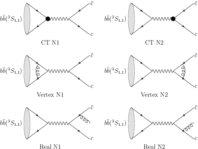
We next consider the QCD radiative corrections. The Feynman diagrams of one-loop virtual corrections and counter terms are shown in Fig. 3. The renormalization of heavy quark wave function should appear. The on-mass-shell (OS) scheme is chosen for Z2​bZ_{2b} and Z2​cZ_{2c}[17]:

δ​Z2​bOS\displaystyle\delta Z_{2b}^{\rm OS} =\displaystyle= −CF​αs4​π​[1ϵUV+2ϵIR−3​γE+3​ln⁡4​π​μ2mb2+4]+𝒪⁡(αs2),\displaystyle-C_{F}\frac{\alpha_{s}}{4\pi}\left[\frac{1}{\epsilon_{\rm UV}}+\frac{2}{\epsilon_{\rm IR}}-3\gamma_{E}+3\ln\frac{4\pi\mu^{2}}{m_{b}^{2}}+4\right]+\mathcal{O}(\alpha_{s}^{2}),
δ​Z2​cOS\displaystyle\delta Z_{2c}^{\rm OS} =\displaystyle= −CF​αs4​π​[1ϵUV+2ϵIR−3​γE+3​ln⁡4​π​μ2mc2+4]+𝒪⁡(αs2),\displaystyle-C_{F}\frac{\alpha_{s}}{4\pi}\left[\frac{1}{\epsilon_{\rm UV}}+\frac{2}{\epsilon_{\rm IR}}-3\gamma_{E}+3\ln\frac{4\pi\mu^{2}}{m_{c}^{2}}+4\right]+\mathcal{O}(\alpha_{s}^{2}), (10)

where μ\mu is the renormalization scale, γE\gamma_{E} is the Euler’s constant. In this scheme, we need not calculate the correction of external quark legs. We employ the two-loop formula for αs​(μ)\alpha_{s}(\mu),

αs​(μ)4​π=1β0​L−β1​ln⁡Lβ03​L2,\frac{\alpha_{s}(\mu)}{4\pi}=\frac{1}{\beta_{0}L}-\frac{\beta_{1}\ln L}{\beta_{0}^{3}L^{2}}, (11)

where L=ln⁡(μ2/ΛQCD2)L=\ln\left(\mu^{2}/\Lambda_{\rm QCD}^{2}\right), and β1=(34/3)​CA2−4​CF​TF​nf−(20/3)​CA​TF​nf\beta_{1}=(34/3){C_{A}}^{2}-4C_{F}T_{F}n_{f}-(20/3)C_{A}T_{F}n_{f} is the two-loop coefficient of the QCD beta function.

The correction to Υ⁡(b​b¯​(S1,13))→γ∗\Upsilon(b\bar{b}({}^{3}S_{1,1}))\to\gamma^{*} gives a factor of −16​αs3​π-\frac{16\alpha_{s}}{3\pi} at 𝒪⁡(αs){\cal O}(\alpha_{s}). The other part is the correction to γ∗→c​c¯\gamma^{*}\to c\bar{c}. If we set mc=0m_{c}=0, then the combined total correction becomes the correction to RR, the ratio of cross section of e+​e−→l​i​g​h​t​h​a​d​r​o​n​se^{+}e^{-}\to light~hadrons to that of e+​e−→μ+​μ−e^{+}e^{-}\to\mu^{+}\mu^{-}. It give a factor of αsπ\frac{\alpha_{s}}{\pi} at 𝒪⁡(αs){\cal O}(\alpha_{s}).

Refer to caption
Figure 3: Feynman diagrams for one-loop QCD corrections with counter terms for b​b¯​(S1,13)→γ∗→c​c¯~b\bar{b}({}^{3}S_{1,1})\to\gamma^{*}\to c\bar{c}

Compared with it, the leptonic width of Υ\Upsilon at 𝒪⁡(αs){\cal O}(\alpha_{s}) becomes the known result:

ΓN​L​O[Υ→e+e−]=2​π​α227​mb2(1−16​αs3​π)⟨Υ|𝒪(S1,13)|Υ⟩.\displaystyle\Gamma_{NLO}[\Upsilon\to e^{+}e^{-}]=\frac{2\pi\alpha^{2}}{27m_{b}^{2}}\left(1-\frac{16\alpha_{s}}{3\pi}\right)\left\langle\Upsilon|{\cal O}({}^{3}S_{1,1})|\Upsilon\right\rangle. (12)

If the parameters are chosen as mb=4.7m_{b}=4.7 GeV, mc=1.5m_{c}=1.5 GeV, and αs=0.220\alpha_{s}=0.220, then the branching ratio is

BN​L​O[Υ(S1,13)→cc¯+X]\displaystyle B_{NLO}[\Upsilon({}^{3}S_{1,1})\to c\bar{c}+X] =\displaystyle= 1.6BN​L​O[Υ→e+e−]≈3.8%.\displaystyle 1.6B_{NLO}[\Upsilon\to e^{+}e^{-}]\approx 3.8\%. (13)

When the emitted gluon energy is large, it would form a jet. So a cut to the gluon energy should be introduced to distinguish between c​c¯c\bar{c} and c​c¯​gc\bar{c}g final states. If Eg<mb×δsE_{g}<m_{b}\times\delta_{s}, the gluon is considered as soft and the final state is c​c¯c\bar{c}. Otherwise, when Eg>mb×δs~E_{g}>m_{b}\times\delta_{s}, the final state is c​c¯​gc\bar{c}g. If we set δs=0.15\delta_{s}=0.15, then the branching ratio is

BN​L​O[Υ(S1,13)→cc¯]\displaystyle B_{NLO}[\Upsilon({}^{3}S_{1,1})\to c\bar{c}] ≈\displaystyle\approx 1.4%.\displaystyle 1.4\%. (14)

If we set δs=0.10\delta_{s}=0.10 and 0.200.20, then the branching ratio is about 5.4×10−35.4\times 10^{-3} and 2.0%2.0\% respectively.

For the color-singlet piece, the contribution of Υ⁡(S1,13)→3​g∗→c​c¯\Upsilon({}^{3}S_{1,1})\to 3g^{*}\to c\bar{c}, which is shown on the right hand side in Fig. 1, has not been calculated so far, and we may have a rough estimate for it. We can use Υ⁡(S1,13)→3​g\Upsilon({}^{3}S_{1,1})\to 3g to give an order of magnitude estimate for the contribution of Υ⁡(S1,13)→3​g∗→c​c¯\Upsilon({}^{3}S_{1,1})\to 3g^{*}\to c\bar{c}. We have the following order of magnitude estimates:

B[Υ(S1,13)→l+l−]\displaystyle B[\Upsilon({}^{3}S_{1,1})\to l^{+}l^{-}] ∝\displaystyle\propto (απ)2,\displaystyle\left(\frac{\alpha}{\pi}\right)^{2},
B[Υ(S1,13)→3g]\displaystyle B[\Upsilon({}^{3}S_{1,1})\to 3g] ∝\displaystyle\propto (αsπ)3,\displaystyle\left(\frac{\alpha_{s}}{\pi}\right)^{3},
B[Υ(S1,13)→ggg∗→ggcc¯]\displaystyle B[\Upsilon({}^{3}S_{1,1})\to ggg^{*}\to ggc\bar{c}] ∝\displaystyle\propto (αsπ)4,\displaystyle\left(\frac{\alpha_{s}}{\pi}\right)^{4},
B[Υ(S1,13)→3g∗→cc¯]\displaystyle B[\Upsilon({}^{3}S_{1,1})\to 3g^{*}\to c\bar{c}] ∝\displaystyle\propto (αsπ)6.\displaystyle\left(\frac{\alpha_{s}}{\pi}\right)^{6}. (15)

Comparing the leptonic width with three-gluon width, we get

Γ[Υ(3S1,1)→l+l−]Γ[Υ(3S1,1)→3g]\displaystyle\frac{\Gamma[\Upsilon({}^{3}S_{1,1})\to l^{+}l^{-}]}{\Gamma[\Upsilon({}^{3}S_{1,1})\to 3g]} ∼\displaystyle\sim (απ)2(αsπ)3∼0.016,\displaystyle\frac{\left(\frac{\alpha}{\pi}\right)^{2}}{\left(\frac{\alpha_{s}}{\pi}\right)^{3}}\sim 0.016, (16)

which is about one half of the experimental value of Γ[Υ(3S1,1)→l+l−]Γ[Υ(3S1,1)→3g]≈0.03\frac{\Gamma[\Upsilon({}^{3}S_{1,1})\to l^{+}l^{-}]}{\Gamma[\Upsilon({}^{3}S_{1,1})\to 3g]}\approx 0.03[50], and the closeness of this estimate to the data may suggest that the naive estimate could make sense. Comparing Υ⁡(S1,13)→3​g∗→c​c¯\Upsilon({}^{3}S_{1,1})\to 3g^{*}\to c\bar{c} with Υ⁡(S1,13)→3​g\Upsilon({}^{3}S_{1,1})\to 3g and Υ⁡(S1,13)→γ∗→c​c¯\Upsilon({}^{3}S_{1,1})\to\gamma^{*}\to c\bar{c}, we can get

Γ[Υ(3S1,1)→3g∗→cc¯]Γ[Υ(3S1,1)→3g]\displaystyle\frac{\Gamma[\Upsilon({}^{3}S_{1,1})\to 3g^{*}\to c\bar{c}]}{\Gamma[\Upsilon({}^{3}S_{1,1})\to 3g]} ∼\displaystyle\sim (αsπ)3≈3×10⁻⁴,\displaystyle\left(\frac{\alpha_{s}}{\pi}\right)^{3}\approx 3\times 10^{-4}, (17)
Γ[Υ(3S1,1)→3g∗→cc¯]Γ[Υ(3S1,1)→γ∗→cc¯]\displaystyle\frac{\Gamma[\Upsilon({}^{3}S_{1,1})\to 3g^{*}\to c\bar{c}]}{\Gamma[\Upsilon({}^{3}S_{1,1})\to\gamma^{*}\to c\bar{c}]} ∼\displaystyle\sim αs6α2​π4≈0.02.\displaystyle\frac{\alpha_{s}^{6}}{\alpha^{2}\pi^{4}}\approx 0.02. (18)

From the estimates given in Eq.(17) and Eq.(18), we see that the contribution of Υ⁡(S1,13)→3​g∗→c​c¯\Upsilon({}^{3}S_{1,1})\to 3g^{*}\to c\bar{c} is very small and much smaller than that of Υ⁡(S1,13)→γ∗→c​c¯\Upsilon({}^{3}S_{1,1})\to\gamma^{*}\to c\bar{c}. Even if the contribution of Υ⁡(S1,13)→3​g∗→c​c¯\Upsilon({}^{3}S_{1,1})\to 3g^{*}\to c\bar{c} is underestimated by an order of magnitude in Eq.(17) and Eq.(18), we could still expect that for the decay Υ⁡(S1,13)→c​c¯\Upsilon({}^{3}S_{1,1})\to c\bar{c} the QED contribution is dominant. Another useful example is the decay rate Γ[Υ(S1,13)→ggcc¯]\Gamma[\Upsilon({}^{3}S_{1,1})\to ggc\bar{c}], which is of higher order in αs\alpha_{s} than Γ[Υ(S1,13)→ggg]\Gamma[\Upsilon({}^{3}S_{1,1})\to ggg], and is given in Ref.[39]. From their estimate we can get Γ[Υ(3S1,1)→ggcc¯]Γ[Υ(3S1,1)→ggg]=0.029\frac{\Gamma[\Upsilon({}^{3}S_{1,1})\to ggc\bar{c}]}{\Gamma[\Upsilon({}^{3}S_{1,1})\to ggg]}=0.029, which is also of the same order of magnitude as, but even smaller than, our naive estimate.

Γ[Υ(3S1,1)→ggcc¯]Γ[Υ(3S1,1)→ggg]\displaystyle\frac{\Gamma[\Upsilon({}^{3}S_{1,1})\to ggc\bar{c}]}{\Gamma[\Upsilon({}^{3}S_{1,1})\to ggg]} ∼\displaystyle\sim (αsπ)≈0.071.\displaystyle\left(\frac{\alpha_{s}}{\pi}\right)\approx 0.071. (19)

This might imply that the naive estimates given in Eq.(15) as well as in Eq.(18) might be tenable in estimating the rates of higher order processes by order of magnitude. So, based on the rough estimate given in Eq.(18) for the contributions of the color-singlet piece to the Υ⁡(S1,13)→c​c¯\Upsilon({}^{3}S_{1,1})\to c\bar{c} process, we assume that, as an approximation, the contribution of Υ⁡(S1,13)→3​g∗→c​c¯\Upsilon({}^{3}S_{1,1})\to 3g^{*}\to c\bar{c} can be neglected, and only Υ⁡(S1,13)→γ∗→c​c¯\Upsilon({}^{3}S_{1,1})\to\gamma^{*}\to c\bar{c} will be taken into consideration.

IV Color octet piece b​b¯​(S1,83)→c​c¯b\bar{b}({}^{3}S_{1,8})\to c\bar{c}

The amplitude of color-octet piece b​b¯​(S1,83)→c​c¯b\bar{b}({}^{3}S_{1,8})\to c\bar{c} can be written as [35, 33]

𝒜⁡(b​b¯​(S1,83​(2​pb)→c⁡(pc)+c¯​(pc¯))CLOSE\displaystyle{\cal A}\Big(b\bar{b}({}^{3}S_{1,8}(2p_{b})\rightarrow c(p_{c})+\bar{c}(p_{\bar{c}})\Big) =\displaystyle= ⟨Υ|𝒪⁡(S1,83)|Υ⟩∑LΥ​z​SΥ​z∑s1​s2∑j​k\displaystyle\sqrt{\left\langle\Upsilon|{\cal O}({}^{3}S_{1,8})|\Upsilon\right\rangle}\sum\limits_{L_{\Upsilon z}S_{\Upsilon z}}\sum\limits_{s_{1}s_{2}}\sum\limits_{jk} (20)
×⟨8a∣3¯k;3j⟩⟨JJz∣LLz;SSz⟩⟨SSz∣s1;s2⟩\displaystyle\hskip-85.35826pt\times\langle 8~a\mid\bar{3}k;3j\rangle\langle JJ_{z}\mid LL_{z};SS_{z}\rangle\langle SS_{z}\mid s_{1};s_{2}\rangle
×𝒜⁡(bj​(pb)+b¯k​(pb)→cl​(pc)+c¯i​(pc¯)),\displaystyle\hskip-85.35826pt\times{\cal A}\Big(b_{j}(p_{b})+\bar{b}_{k}(p_{b})\rightarrow c_{l}(p_{c})+\bar{c}_{i}(p_{\bar{c}})\Big),

where ⟨8a∣3¯k;3j⟩=2Tj​ka\langle 8~a\mid\bar{3}k;3j\rangle=\sqrt{2}T^{a}_{jk}, and other expressions are similar to the color-singlet piece.

The Born diagram of b​b¯​(S1,83)→c​c¯b\bar{b}({}^{3}S_{1,8})\to c\bar{c} is shown in Fig. 2. It is also calculated in Ref. [32]. The leading order width is

ΓL​O[Υ(S1,83)→cc¯]=αs2​1−r2​(2+r2)​π6​mb2⟨Υ|𝒪(S1,83)|Υ⟩.\displaystyle\Gamma_{LO}[\Upsilon({}^{3}S_{1,8})\to c\bar{c}]=\frac{\alpha_{s}^{2}\sqrt{1-r^{2}}\left(2+r^{2}\right)\pi}{6m_{b}^{2}}\left\langle\Upsilon|{\cal O}({}^{3}S_{1,8})|\Upsilon\right\rangle. (21)

We further calculate the next-to-leading order (NLO) corrections. The Feynman diagrams for NLO virtual corrections with counter terms in the color-octet piece b​b¯​(S1,83)→c​c¯b\bar{b}({}^{3}S_{1,8})\to c\bar{c} are shown in Fig. 4. The Feynman diagrams for NLO real corrections in the color-octet piece b​b¯​(S1,83)→c​c¯b\bar{b}({}^{3}S_{1,8})\to c\bar{c} are shown in Fig. 5. The renormalization of heavy quark wave function, gluon wave function, and coupling constant should appear here. Z2​bZ_{2b} and Z2​cZ_{2c} are given in Eq. (10). For Z3Z_{3} and ZgZ_{g}, we choose the modified minimal-subtraction (MS¯~\overline{\rm MS} ) scheme[17]:

δ​Z3MS¯\displaystyle\delta Z_{3}^{\overline{\rm MS}} =\displaystyle= αs4​π​(β0−2​CA)​[1ϵUV−γE+ln⁡(4​π)]+𝒪⁡(αs2),\displaystyle\frac{\alpha_{s}}{4\pi}(\beta_{0}-2C_{A})\left[\frac{1}{\epsilon_{\rm UV}}-\gamma_{E}+\ln(4\pi)\right]+\mathcal{O}(\alpha_{s}^{2}),
δ​ZgMS¯\displaystyle\delta Z_{g}^{\overline{\rm MS}} =\displaystyle= −β02​αs4​π​[1ϵUV−γE+ln⁡(4​π)]+𝒪⁡(αs2).\displaystyle-\frac{\beta_{0}}{2}\,\frac{\alpha_{s}}{4\pi}\left[\frac{1}{\epsilon_{\rm UV}}-\gamma_{E}+\ln(4\pi)\right]+\mathcal{O}(\alpha_{s}^{2}). (22)
Refer to caption
Figure 4: Feynman diagrams for next-to-leading order virtual corrections with counter terms in the color-octet piece b​b¯​(S1,83)→c​c¯b\bar{b}({}^{3}S_{1,8})\to c\bar{c}
Refer to caption
Figure 5: Feynman diagrams for next-to-leading order real corrections in the color-octet piece b​b¯​(S1,83)→c​c¯b\bar{b}({}^{3}S_{1,8})\to c\bar{c}

The parameters are chosen as mb=4.7m_{b}=4.7 GeV, mc=1.5m_{c}=1.5 GeV, nf=4n_{f}=4, ΛQ​C​D(4)=338\Lambda_{QCD}^{(4)}=338 MeV, μ=mb\mu=m_{b}, and then αs=0.220\alpha_{s}=0.220. So we can get the leading order result:

BL​O[Υ(S1,83)→cc¯]\displaystyle B_{LO}[\Upsilon({}^{3}S_{1,8})\to c\bar{c}] =\displaystyle= 42×⟨Υ|𝒪⁡(S1,83)|Υ⟩GeV3.\displaystyle 42\times\frac{\left\langle\Upsilon|{\cal O}({}^{3}S_{1,8})|\Upsilon\right\rangle}{\rm GeV^{3}}. (23)

The total NLO result is

BN​L​O[Υ(S1,83)→cc¯+X]\displaystyle B_{NLO}[\Upsilon({}^{3}S_{1,8})\to c\bar{c}+X] =\displaystyle= 53×⟨Υ|𝒪⁡(S1,83)|Υ⟩GeV3.\displaystyle 53\times\frac{\left\langle\Upsilon|{\cal O}({}^{3}S_{1,8})|\Upsilon\right\rangle}{\rm GeV^{3}}. (24)

If we set the soft cut δs=0.15~\delta_{s}=0.15, then the NLO result is

BN​L​O[Υ(S1,83)→cc¯]\displaystyle B_{NLO}[\Upsilon({}^{3}S_{1,8})\to c\bar{c}] =\displaystyle= 41×⟨Υ|𝒪⁡(S1,83)|Υ⟩GeV3.\displaystyle 41\times\frac{\left\langle\Upsilon|{\cal O}({}^{3}S_{1,8})|\Upsilon\right\rangle}{\rm GeV^{3}}. (25)

If we set the soft cut δs=0.10\delta_{s}=0.10 and 0.200.20, then the branching ratio is 37×⟨Υ|𝒪⁡(S1,83)|Υ⟩GeV337\times\frac{\left\langle\Upsilon|{\cal O}({}^{3}S_{1,8})|\Upsilon\right\rangle}{\rm GeV^{3}} and 44×⟨Υ|𝒪⁡(S1,83)|Υ⟩GeV344\times\frac{\left\langle\Upsilon|{\cal O}({}^{3}S_{1,8})|\Upsilon\right\rangle}{\rm GeV^{3}} respectively.

From the above expressions, we see that the short-distance coefficient for this color-octet process is large, and this color-octet process may make a significant contribution to the Υ\Upsilon decay to two-charm quark jet. The numerical estimate will be given in the next section.

The color-octet pieces b​b¯​(PJ,83)b\bar{b}({}^{3}P_{J,8}) and b​b¯​(S0,81)b\bar{b}({}^{1}S_{0,8}) also contribute to the charm quark jet production through c​c¯​gc\bar{c}g, where the gluon is soft. The b​b¯​(PJ,83)→c​c¯​gb\bar{b}({}^{3}P_{J,8})\to c\bar{c}g is IR divergent, and it should be absorbed into the matrix element ⟨Υ|𝒪⁡(S1,83)|Υ⟩\left\langle\Upsilon|{\cal O}({}^{3}S_{1,8})|\Upsilon\right\rangle [1]:

⟨Υ​|𝒪⁡(S1,83)|​Υ⟩1\displaystyle\left\langle\Upsilon\left|{\cal O}\left({}^{3}\!S_{1,8}\right)\right|\Upsilon\right\rangle_{1} =\displaystyle= ⟨Υ​|𝒪H​(S1,83)|​Υ⟩0​[1+(CF−CA2)​π​αs2​v]+4​αs3​π​mb2​(4​π​μ2λ2)ϵ\displaystyle\left\langle\Upsilon\left|{\cal O}^{H}\left({}^{3}\!S_{1,8}\right)\right|\Upsilon\right\rangle_{0}\left[1+\left(C_{F}-\frac{C_{A}}{2}\right)\frac{\pi\alpha_{s}}{2v}\right]+\frac{4\alpha_{s}}{3\pi m_{b}^{2}}\left(\frac{4\pi\mu^{2}}{\lambda^{2}}\right)^{\epsilon} (26)
×exp⁡(−ϵ​γE)​(1ϵUV−1ϵIR)​∑J=02BF​⟨Υ​|𝒪⁡(PJ,83)|​Υ⟩,\displaystyle{}\times\exp(-\epsilon\gamma_{E})\left(\frac{1}{\epsilon_{\rm UV}}-\frac{1}{\epsilon_{\rm IR}}\right)\sum_{J=0}^{2}B_{F}\left\langle\Upsilon\left|{\cal O}\left({}^{3}\!P_{J,8}\right)\right|\Upsilon\right\rangle,

where the Coulomb term of ⟨Υ​|𝒪⁡(S1,83)|​Υ⟩1\left\langle\Upsilon\left|{\cal O}\left({}^{3}\!S_{1,8}\right)\right|\Upsilon\right\rangle_{1} is canceled by the virtual correction, the IR divergent terms is canceled by b​b¯​(PJ,83)→c​c¯​gb\bar{b}({}^{3}P_{J,8})\to c\bar{c}g, and the UV divergent term gives the running of matrix element. If we choose the matrix element renormalization scale as mbm_{b}, then we find the branching ratio of b​b¯​(PJ,83)b\bar{b}({}^{3}P_{J,8}) and b​b¯​(S0,81)b\bar{b}({}^{1}S_{0,8}) decays into c​c¯​gc\bar{c}g at order of αs3\alpha_{s}^{3} to be

B[Υ(S0,81)→cc¯+X]\displaystyle B[\Upsilon({}^{1}S_{0,8})\to c\bar{c}+X] =\displaystyle= 2.8×⟨Υ|𝒪⁡(S0,81)|Υ⟩GeV3,\displaystyle 2.8\times\frac{\left\langle\Upsilon|{\cal O}({}^{1}S_{0,8})|\Upsilon\right\rangle}{\rm GeV^{3}},
B[Υ(PJ,83)→cc¯+X]\displaystyle B[\Upsilon({}^{3}P_{J,8})\to c\bar{c}+X] =\displaystyle= 0.61×⟨Υ|𝒪⁡(P0,83)|Υ⟩GeV5.\displaystyle 0.61\times\frac{\left\langle\Upsilon|{\cal O}({}^{3}P_{0,8})|\Upsilon\right\rangle}{\rm GeV^{5}}. (27)

Since ⟨Υ|𝒪⁡(S0,81)|Υ⟩\left\langle\Upsilon|{\cal O}({}^{1}S_{0,8})|\Upsilon\right\rangle, ⟨Υ|𝒪⁡(S1,83)|Υ⟩\left\langle\Upsilon|{\cal O}({}^{3}S_{1,8})|\Upsilon\right\rangle, and ⟨Υ|𝒪⁡(PJ,83)|Υ⟩/mb2\left\langle\Upsilon|{\cal O}({}^{3}P_{J,8})|\Upsilon\right\rangle/m_{b}^{2} are of the same order , we can ignore the contribution of b​b¯​(PJ,83)b\bar{b}({}^{3}P_{J,8}) and b​b¯​(S0,81)b\bar{b}({}^{1}S_{0,8}), as compared with the b​b¯​(S1,83)b\bar{b}({}^{3}S_{1,8}) contribution given in Eq.(24).

Refer to caption
Figure 6: Decay widths of the color-singlet piece and color-octet piece b​b¯​(S13)→c​c¯b\bar{b}({}^{3}S_{1})\to c\bar{c} rescaled by the corresponding value at mc=1.5m_{c}=1.5~GeV as functions of the charm quark mass mcm_{c}. Here Λ=0.338​GeV\Lambda=0.338{\rm GeV}, mb=4.7​GeVm_{b}=4.7~{\rm GeV}, μ=mb\mu=m_{b}, and the soft cut δs=0.15\delta_{s}=0.15. LO means leading order, and NLO means next-to-leading order. S1,13{}^{3}S_{1,1} means the ratio Γ[bb¯(S1,13→cc¯](mc)/Γ[bb¯(S1,13→cc¯](mc=1.5GeV)\Gamma[b\bar{b}({}^{3}S_{1,1}\to c\bar{c}](m_{c})/\Gamma[b\bar{b}({}^{3}S_{1,1}\to c\bar{c}](m_{c}=1.5~{\rm GeV}) in the color-singlet piece, and S1,83{}^{3}S_{1,8} means the corresponding ratio in the color-octet piece.

The dependence of the leading order and next-to-leading order decay widths in the color-singlet and color-octet pieces b​b¯→c​c¯b\bar{b}\to c\bar{c} on the charm quark is shown in Fig. 6. The dependence of LO result on the charm quark mass is weak and the same for the color-singlet and color-octet pieces. The reason can be found in Eq. (6) and Eq. (21). If we choose mc=1.5±0.2m_{c}=1.5\pm 0.2~GeV, the ratio is about 1±0.0031\pm 0.003 at LO in αs\alpha_{s}, 1−0.30+0.271^{+0.27}_{-0.30} at NLO for the color-singlet piece, and 1−0.057+0.0461^{+0.046}_{-0.057} at NLO for the color-octet piece.

Refer to caption
Figure 7: Decay widths of the color-singlet piece and color-octet piece b​b¯​(S13)→c​c¯b\bar{b}({}^{3}S_{1})\to c\bar{c} rescaled by the corresponding value at μ=mb\mu=m_{b} as functions of the renormalization scale μ\mu. Here Λ=0.338​GeV\Lambda=0.338{\rm GeV}, mb=4.7​GeVm_{b}=4.7~{\rm GeV}, mc=1.5m_{c}=1.5~GeV, and the soft cut δs=0.15\delta_{s}=0.15. LO means leading order, and NLO means next-to-leading order. S1,13{}^{3}S_{1,1} means the ratio of Γ[bb¯(S1,13→cc¯](μ)/Γ[bb¯(S1,13→cc¯](μ=mb)\Gamma[b\bar{b}({}^{3}S_{1,1}\to c\bar{c}](\mu)/\Gamma[b\bar{b}({}^{3}S_{1,1}\to c\bar{c}](\mu=m_{b}) in the color-singlet piece, and S1,83{}^{3}S_{1,8} means the corresponding ratio in the color-octet piece.

The dependence of the leading order and next-to-leading order decay widths in the color-singlet and color-octet pieces b​b¯→c​c¯b\bar{b}\to c\bar{c} on the renormalization scale μ\mu is shown in Fig. 7. The LO color-singlet result is independent of the renormalization scale. As it is shown in the curve of NLO S1,83{}^{3}S_{1,8}, we choose μ=mb\mu=m_{b} for the ¡°principle of minimum sensitivity¡±(PMS) [51].

Refer to caption
Figure 8: Decay widths of the color-singlet piece and color-octet piece b​b¯​(S13)→c​c¯b\bar{b}({}^{3}S_{1})\to c\bar{c} rescaled by the corresponding value at δs=0.15\delta_{s}=0.15 as functions of the soft cut δs\delta_{s}. Here Λ=0.338​GeV\Lambda=0.338{\rm GeV}, mb=4.7​GeVm_{b}=4.7~{\rm GeV}, μ=mb\mu=m_{b}, and mc=1.5m_{c}=1.5~GeV. NLO means next-to-leading order. S1,13{}^{3}S_{1,1} means the ratio of Γ[bb¯(S1,13→cc¯](δs)/Γ[bb¯(S1,13→cc¯](δs=0.15)\Gamma[b\bar{b}({}^{3}S_{1,1}\to c\bar{c}](\delta_{s})/\Gamma[b\bar{b}({}^{3}S_{1,1}\to c\bar{c}](\delta_{s}=0.15), and S1,83{}^{3}S_{1,8} means the corresponding ratio in the color-octet piece.

The dependence of the next-to-leading order decay widths in the color-singlet and color-octet pieces b​b¯→c​c¯b\bar{b}\to c\bar{c} on the soft cut δs\delta_{s} is shown in Fig. 8. The LO result is independent of the soft cut δs\delta_{s}. The NLO color-singlet result is rather sensitive to δs\delta_{s}, whereas the NLO color-octet result is insensitive to δs\delta_{s}.

V Color octet matrix elements

The color-singlet matrix element ⟨Υ|𝒪⁡(S1,13)|Υ⟩\left\langle\Upsilon|{\cal O}({}^{3}S_{1,1})|\Upsilon\right\rangle can be extracted from the Υ\Upsilon leptonic decay width. Using Eq. (12), we get

⟨Υ|𝒪⁡(S1,13)|Υ⟩=3.8​GeV3.\displaystyle\left\langle\Upsilon|{\cal O}({}^{3}S_{1,1})|\Upsilon\right\rangle=3.8~{\rm GeV^{3}}. (28)

On the other hand, large uncertainty is related to the color octet matrix element ⟨Υ|𝒪⁡(S1,83)|Υ⟩\left\langle\Upsilon|{\cal O}({}^{3}S_{1,8})|\Upsilon\right\rangle. According to the velocity scaling rule and taking v2=0.08v^{2}=0.08, we might naively have

⟨Υ|𝒪⁡(S1,83)|Υ⟩\displaystyle\left\langle\Upsilon|{\cal O}({}^{3}S_{1,8})|\Upsilon\right\rangle ≈\displaystyle\approx v42​Nc​⟨Υ|𝒪⁡(S1,13)|Υ⟩=4.1×10⁻³​GeV3.\displaystyle\frac{v^{4}}{2N_{c}}\left\langle\Upsilon|{\cal O}({}^{3}S_{1,1})|\Upsilon\right\rangle=4.1\times 10^{-3}~{\rm GeV^{3}}. (29)

Using Eq. (24), we would get

BN​L​O[Υ(S1,83)→cc¯+X]\displaystyle B_{NLO}[\Upsilon({}^{3}S_{1,8})\to c\bar{c}+X] =\displaystyle= 21%.\displaystyle 21\%. (30)

For the light quark q=u,d,sq=u,d,s, we have

BN​L​O[Υ(S1,83)→qq¯+X]=BN​L​O[Υ(S1,83)→cc¯+X]×(1+𝒪(r2)).\displaystyle B_{NLO}[\Upsilon({}^{3}S_{1,8})\to q\bar{q}+X]=B_{NLO}[\Upsilon({}^{3}S_{1,8})\to c\bar{c}+X]\times\left(1+{\cal O}\left(r^{2}\right)\right). (31)

So Υ\Upsilon decay through b​b¯​(S1,83)b\bar{b}({}^{3}S_{1,8}) would have a very large branching ratio, say about 80%~80\%. Apparently, the color -octet matrix element estimated in this naive way from the velocity scaling rule is greatly overestimated, even by an order of magnitude.

Another approach to determine the matrix element is the lattice QCD calculations. The lattice calculation in Ref. [52] gives

⟨Υ|𝒪⁡(S1,83)|Υ⟩\displaystyle\left\langle\Upsilon|{\cal O}({}^{3}S_{1,8})|\Upsilon\right\rangle ≈\displaystyle\approx 8.1×10⁻⁵​⟨Υ|𝒪⁡(S1,13)|Υ⟩=3.1×10⁻⁴​GeV3.\displaystyle 8.1\times 10^{-5}\left\langle\Upsilon|{\cal O}({}^{3}S_{1,1})|\Upsilon\right\rangle=3.1\times 10^{-4}~{\rm GeV^{3}}. (32)

If we set the soft cut δs=0.15\delta_{s}=0.15, then the next-to-leading order result is

BN​L​O[Υ(S1,83)→cc¯]\displaystyle B_{NLO}[\Upsilon({}^{3}S_{1,8})\to c\bar{c}] =\displaystyle= 1.3%.\displaystyle 1.3\%. (33)

If we set the soft cut δs=0.10\delta_{s}=0.10 and δs=0.20\delta_{s}=0.20, the branching ratio is 1.1%1.1\% and 1.4%1.4\% respectively.

From the above numerical results and Eq.(24) we see that since the short distance coefficient for the color-octet contribution to the Υ→c​c¯\Upsilon\to c\bar{c} decay is large, this process is sensitive to the value of the color-octet matrix element, and may therefore serve as a useful test ground of the color-octet mechanism.

Moreover, the next-to-leading order QCD correction in the color-singlet piece is much stronger than that in the color-octet piece, and the color-singlet contribution shows a strong sensitivity to the soft cut δs\delta_{s}, whereas the color-octet result does not. These differences between the color-singlet and color-octet contributions will also be significant in clarifying the issue about the color-octet mechanism. Once the experiment can measure the branching ratio and energy distribution of the charm quark jet in the Υ\Upsilon decay, the result can be used to test the color-octet mechanism or give a strong constraint on the color-octet matrix elements.

VI Summary and discussion

We calculate the decay rate of bottomonium to two-charm quark jets Υ→c​c¯\Upsilon\to c\bar{c} at the tree level and one-loop level including color-singlet and color-octet b​b¯b\bar{b} annihilations. We find that the short distance coefficient of the color-octet piece is much larger than the color-singlet piece, and that the QCD correction will change the endpoint behavior of the charm quark jet. The color-singlet piece is strongly affected by the one-loop QCD correction. In contrast, the QCD correction to the color-octet piece is weak. Once the experiment can measure the branching ratio and energy distribution of the two-charm quark jets in the Υ\Upsilon decay, the result can be used to test the color octet mechanism or give a strong constraint on the color-octet matrix elements.

After our work was completed [53], a paper appeared [39], in which Kang, Kim, Lee, and Yu calculated the inclusive charm production in Υ⁡(n​S)\Upsilon(nS) decay. They focused on the inclusive charm production of the color-singlet piece at leading order in the strong coupling constant αs\alpha_{s}. We focused on the c​c¯c\bar{c} final state and the color-octet mechanism. The c​c¯c\bar{c} final state is essentially the two charm-jet process. And we have calculated the next-to-leading order QCD corrections in both color singlet and color octet pieces. Our leading order result of Υ→γ∗→c​c¯\Upsilon\to\gamma^{*}\to c\bar{c} is consistent with their result [39].

Acknowledgements.
We thank C. Meng for useful discussions. This work was supported in part by the National Natural Science Foundation of China (No 10421503, No 10675003), and also by China Postdoctoral Science Foundation (No 20070420011).

APPENDICES

Appendix A The scalar functions

The scalar functions that appear in the virtual corrections are listed in this Appendix. There are UV, IR and Coulomb singularities in the scalar functions. The UV and IR singularities are regularized with D=4−2​ϵD=4-2\epsilon space-time dimension. The exchange of longitudinal gluon between massive quarks in Vertex N1 in Fig.3 and Fig.4 leads to a Coulomb singularity ∼π2/v\sim\pi^{2}/v, where v=−(pb−pb¯)2/mbv=\sqrt{-(p_{b}-p_{\bar{b}})^{2}}/m_{b} is the relative velocity between bb and b¯\bar{b} in the meson rest frame (v=|pb→−pb¯→|/mbv=|\overrightarrow{p_{b}}-\overrightarrow{p_{\bar{b}}}|/m_{b}). The Coulomb singularities should be canceled by that in the matrix elements (see, e.g., [17, 16]).

Since the imaginary part of the integrals will disappear in the final result, only the real parts are given. The external particles are taken to be on-mass-shell, pb2=pb¯2=mb2p_{b}^{2}=p_{\bar{b}}^{2}=m_{b}^{2}, pc2=pc¯2=mc2p_{c}^{2}=p_{\bar{c}}^{2}=m_{c}^{2}, pb⋅pc=pb⋅pc¯=mb2p_{b}\cdot p_{c}=p_{b}\cdot p_{\bar{c}}=m_{b}^{2}, and pc⋅pc¯=2​mb2−mc2p_{c}\cdot p_{\bar{c}}=2m_{b}^{2}-m_{c}^{2}.

The scalar one-point function is defined as

A0​(m2)=μ4−D​∫dD​q(2​π)D​1q2−m2=i​Cϵ​(m)​m2​[1ϵ+1]\displaystyle A_{0}(m^{2})=\mu^{4-D}\;\int\frac{\mbox{d}^{D}q}{(2\pi)^{D}}\;\frac{1}{q^{2}-m^{2}}=iC_{\epsilon}(m)\;m^{2}\,\left[\,\frac{1}{\epsilon}+1\,\right] (34)

where

Cϵ​(m)=116​π2​e−ϵ⁡(γE−ln⁡4​π)​(μ2m2)ϵ\displaystyle C_{\epsilon}(m)=\frac{1}{16\pi^{2}}\;\;e^{-\epsilon(\gamma_{E}-\ln 4\pi)}\left(\frac{\mu^{2}}{m^{2}}\right)^{\epsilon} (35)

and D=4−2​ϵD=4-2\epsilon.

The scalar two-point function is defined as

B0​(p,m0,m1)=μ4−D​∫dD​q(2​π)D​1[q2−m02]​[(q+p)2−m12]\displaystyle B_{0}(p,m_{0},m_{1})=\mu^{4-D}\;\int\frac{\mbox{d}^{D}q}{(2\pi)^{D}}\;\frac{1}{[q^{2}-m_{0}^{2}]\,[(q+p)^{2}-m_{1}^{2}]}\quad (36)

Four different types of two-point functions appear in the calculation of the virtual corrections:

B0​(pb,0,mb)\displaystyle B_{0}(p_{b},0,m_{b}) =\displaystyle= B0​(2​pb,mb,mb)=i​Cϵ​(mb)​[1ϵ+2]\displaystyle B_{0}(2p_{b},m_{b},m_{b})=iC_{\epsilon}(m_{b})\;\left[\,\frac{1}{\epsilon}+2\,\right] (37)
B0​(pc,0,mc)\displaystyle B_{0}(p_{c},0,m_{c}) =\displaystyle= B0​(pc¯,0,mc)=i​Cϵ​(mc)​[1ϵ+2]\displaystyle B_{0}(p_{\bar{c}},0,m_{c})=iC_{\epsilon}(m_{c})\;\left[\,\frac{1}{\epsilon}+2\,\right] (38)
B0​(2​pb,mc,mc)\displaystyle B_{0}(2p_{b},m_{c},m_{c}) =\displaystyle= i​Cϵ​(mc)​[1ϵ+2+β​ln⁡(1−β1+β)]\displaystyle iC_{\epsilon}(m_{c})\;\left[\,\frac{1}{\epsilon}+2+\beta\ln\left(\frac{1-\beta}{1+\beta}\right)\right] (39)
B0​(pc−pb,mc,mb)\displaystyle B_{0}(p_{c}-p_{b},m_{c},m_{b}) =\displaystyle= i​Cϵ​(mc)​[1ϵ+2+1β​ln⁡(1−β1+β)]\displaystyle iC_{\epsilon}(m_{c})\;\left[\,\frac{1}{\epsilon}+2+\frac{1}{\beta}\ln\left(\frac{1-\beta}{1+\beta}\right)\right] (40)
B0​(2​pb,0,0)\displaystyle B_{0}(2p_{b},0,0) =\displaystyle= i​Cϵ​(mc)​[1ϵ−ln⁡(4​mb2mc2)+2].\displaystyle iC_{\epsilon}(m_{c})\;\left[\,\frac{1}{\epsilon}-\ln\left(\frac{4m_{b}^{2}}{m_{c}^{2}}\right)+2\right]. (41)

Here and below we will use the shorthand notation β=1−r2=1−mc2/mb2\beta=\sqrt{1-r^{2}}=\sqrt{1-m_{c}^{2}/m_{b}^{2}}.

The scalar three-point function is defined as

C0​(p1,p2,m0,m1,m2)=\displaystyle\hskip-28.45274ptC_{0}(p_{1},p_{2},m_{0},m_{1},m_{2})= (42)
μ4−D​∫dD​q(2​π)D​1[q2−m02]​[(q+p1)2−m12]​[(q+p2)2−m22].\displaystyle\mu^{4-D}\;\int\frac{\mbox{d}^{D}q}{(2\pi)^{D}}\;\frac{1}{[q^{2}-m_{0}^{2}]\,[(q+p_{1})^{2}-m_{1}^{2}]\,[(q+p_{2})^{2}-m_{2}^{2}]}\quad.

The following types of three-point functions appear in the virtual corrections:

C0​(pc,−pc¯,0,mc,mc)\displaystyle C_{0}(p_{c},-p_{\bar{c}},0,m_{c},m_{c}) =\displaystyle= i​Cϵ​(mc)4​mb2​β[1ϵlnxβ−2lnxβln(1−xβ)−2Li2(xβ)\displaystyle\frac{iC_{\epsilon}(m_{c})}{4m_{b}^{2}\beta}\left[\frac{1}{\epsilon}\ln x_{\beta}-2\ln x_{\beta}\ln(1-x_{\beta})-2{{\mbox{Li}}}_{2}(x_{\beta})\right. (43)
+12ln2xβ−4ζ(2)]\displaystyle\hskip 14.22636pt\left.+\frac{1}{2}\ln^{2}x_{\beta}-4\zeta(2)\right]
C0​(pc,pb,0,mc,mb)\displaystyle C_{0}(p_{c},p_{b},0,m_{c},m_{b}) =\displaystyle= i​Cϵ​(mc​mb)4​mc​mb​χ/(χ2−1)[1ϵln(1−χχ+1)+12ln2(1−χχ+1)−ln2⁡r2\displaystyle\frac{iC_{\epsilon}(\sqrt{m_{c}m_{b}})}{4m_{c}m_{b}\chi/(\chi^{2}-1)}\left[\frac{1}{\epsilon}\ln\left(\frac{1-\chi}{\chi+1}\right)+\frac{1}{2}\ln^{2}\left(\frac{1-\chi}{\chi+1}\right)-\frac{\ln^{2}r}{2}\right. (44)
−2​ln⁡(4​χ(χ+1)2)​ln⁡(1−χχ+1)−Li2​((χ−1)2(χ+1)2)\displaystyle\hskip 14.22636pt\left.-2\ln\left(\frac{4\chi}{(\chi+1)^{2}}\right)\ln\left(\frac{1-\chi}{\chi+1}\right)-\text{Li}_{2}\left(\frac{(\chi-1)^{2}}{(\chi+1)^{2}}\right)\right.
−Li2(1+r⁡(χ−1)χ+1)−Li2(1+χ−1r⁡(χ+1))+π26]\displaystyle\hskip 14.22636pt\left.-\text{Li}_{2}\left(1+\frac{r(\chi-1)}{\chi+1}\right)-\text{Li}_{2}\left(1+\frac{\chi-1}{r(\chi+1)}\right)+\frac{\pi^{2}}{6}\right]
C0​(pc,−pc¯,mc,0,0)\displaystyle C_{0}(p_{c},-p_{\bar{c}},m_{c},0,0) =\displaystyle= i​14​(4​π)2​mb2​β​[2​Li2​(−xβ)+12​ln2​xβ+ζ⁡(2)]\displaystyle i\frac{1}{4(4\pi)^{2}m_{b}^{2}\beta}\left[2{{\mbox{Li}}}_{2}(-x_{\beta})+\frac{1}{2}\ln^{2}x_{\beta}+\zeta(2)\right] (45)
C0​(pb,−pb,mb,0,0)\displaystyle C_{0}(p_{b},-p_{b},m_{b},0,0) =\displaystyle= i​ln⁡2(4​π)2​mb2,\displaystyle i\frac{\ln 2}{(4\pi)^{2}m_{b}^{2}}, (46)

where xβ=(1−β)/(1+β)x_{\beta}=(1-\beta)/(1+\beta) , ζ⁡(2)=π2/6\zeta(2)=\pi^{2}/6, r=mc/mbr=m_{c}/m_{b}, and χ=(1−r)/(1+r)\chi=\sqrt{(1-r)/(1+r)}. There is another scalar three-point function that is IR and Coulomb divergent,

C0​(pb,−pb¯,0,mb,mb)\displaystyle C_{0}(p_{b},-p_{\bar{b}},0,m_{b},m_{b}) =\displaystyle= −i​Cϵ​(mb)2​mb2​[1ϵ+π2v−2+𝒪⁡(ϵ)]\displaystyle-i\frac{C_{\epsilon}(m_{b})}{2m_{b}^{2}}\left[\,\frac{1}{\epsilon}+\frac{\pi^{2}}{v}-2+{\cal O}(\epsilon)\right] (47)

where v=−(pb−pb¯)2/mbv=\sqrt{-(p_{b}-p_{\bar{b}})^{2}}/m_{b}. In the meson rest frame, we have v=|pb→−pb¯→|/mbv=|\overrightarrow{p_{b}}-\overrightarrow{p_{\bar{b}}}|/m_{b}.

The scalar four-point function is defined by

D0​(p1,p2,p3,m0,m1,m2,m3)=\displaystyle\hskip-36.98866ptD_{0}(p_{1},p_{2},p_{3},m_{0},m_{1},m_{2},m_{3})=
μ4−D​∫dD​q(2​π)D​1[q2−m02]​[(q+p1)2−m12]​[(q+p2)2−m22]​[(q+p3)2−m32].\displaystyle\hskip-28.45274pt\mu^{4-D}\;\int\frac{\mbox{d}^{D}q}{(2\pi)^{D}}\;\frac{1}{[q^{2}-m_{0}^{2}]\,[(q+p_{1})^{2}-m_{1}^{2}]\,[(q+p_{2})^{2}-m_{2}^{2}]\,[(q+p_{3})^{2}-m_{3}^{2}]}\quad. (48)

There are three different types of four-point functions:

D0​(pb,pb−pc,−pb,mb,0,mc,0)\displaystyle D_{0}(p_{b},p_{b}-p_{c},-p_{b},m_{b},0,m_{c},0) (49)
=\displaystyle= i​Cϵ​(mc​mb)8​mb4{(χ2−1)r​χ[1ϵln(1−χχ+1)+12ln2(1−χχ+1)−ln2⁡r2\displaystyle\frac{iC_{\epsilon}(\sqrt{m_{c}m_{b}})}{8m_{b}^{4}}\left\{\frac{(\chi^{2}-1)}{r\chi}\left[\frac{1}{\epsilon}\ln\left(\frac{1-\chi}{\chi+1}\right)+\frac{1}{2}\ln^{2}\left(\frac{1-\chi}{\chi+1}\right)-\frac{\ln^{2}r}{2}\right.\right.
−2​ln⁡(4​χ(χ+1)2)​ln⁡(1−χχ+1)−Li2​((χ−1)2(χ+1)2)−Li2​(1+r⁡(χ−1)χ+1)\displaystyle\left.-2\ln\left(\frac{4\chi}{(\chi+1)^{2}}\right)\ln\left(\frac{1-\chi}{\chi+1}\right)-\text{Li}_{2}\left(\frac{(\chi-1)^{2}}{(\chi+1)^{2}}\right)-\text{Li}_{2}\left(1+\frac{r(\chi-1)}{\chi+1}\right)\right.
−Li2(1+χ−1r⁡(χ+1))+π26]−1β[2Li2(−xβ)+12ln2xβ+ζ(2)]},\displaystyle\left.\left.-\text{Li}_{2}\left(1+\frac{\chi-1}{r(\chi+1)}\right)+\frac{\pi^{2}}{6}\right]-\frac{1}{\beta}\left[2{{\mbox{Li}}}_{2}(-x_{\beta})+\frac{1}{2}\ln^{2}x_{\beta}+\zeta(2)\right]\right\},

The IR and Coulomb singularities can be regularized by the gluon mass mgm_{g}. The relation between the gluon mass mgm_{g} regularization and the dimensional regularization for IR singularity is

ln⁡(λ2m2)⟺1ϵ−γE+ln⁡4​π​μ2m2\displaystyle\ln\left(\frac{\lambda^{2}}{m^{2}}\right)\Longleftrightarrow\frac{1}{\epsilon}-\gamma_{\mathrm{E}}+\ln\frac{4\pi\mu^{2}}{m^{2}} (50)

And the relation between different regularization schemes for the Coulomb singularity is

2​π​mλ⟺π2v\displaystyle\frac{2\pi m}{\lambda}\Longleftrightarrow\frac{\pi^{2}}{v} (51)

Eq.(50) and Eq.(51) are consistent with Ref.[2].

Appendix B Real corrections and the three-body phase space

For the real corrections, the process Υ⁡(2​pb)→c⁡(pc)+c¯​(pc¯)+g⁡(k)\Upsilon(2p_{b})\to c(p_{c})+\bar{c}(p_{\bar{c}})+g(k) is a three-body decay process. Similar to the method in Ref. [47], we can write down the Lorentz-invariant phase space

dPS3​(2​pb,k,pc,pc¯)\displaystyle\rm dPS_{3}(2p_{b};k,p_{c},p_{\bar{c}}) =\displaystyle= d3​k(2​π)3​2​k0​d3​pc(2​π)3​2​pc0​d3​pc¯(2​π)3​2​pc¯0​(2​π)4​δ4​(2​pb−k−pc−pc¯).\displaystyle\frac{\rm d^{3}k}{(2\pi)^{3}2k^{0}}\frac{\rm d^{3}p_{c}}{(2\pi)^{3}2p_{c}^{0}}\frac{\rm d^{3}p_{\bar{c}}}{(2\pi)^{3}2p_{\bar{c}}^{0}}(2\pi)^{4}\delta^{4}(2p_{b}-k-p_{c}-p_{\bar{c}}). (52)

Introduce the identities

d3​pi2​pi0=d4​pi​δ​(pi2−mi2)=|pi→|2​d​|pi→|​d​Ωi2​pi0=|pi→|​dpi0​d​Ωi2,\displaystyle\frac{\rm d^{3}p_{i}}{2p_{i}^{0}}=\rm d^{4}p_{i}\delta(p_{i}^{2}-m_{i}^{2})={\rm\frac{|\overrightarrow{p_{i}}|^{2}\ d|\overrightarrow{p_{i}}|\ d\Omega_{i}}{2p_{i}^{0}}}={\rm\frac{|\overrightarrow{p_{i}}|\ dp_{i}^{0}\ d\Omega_{i}}{2}}, (53)

where mim_{i} is the mass of particle ii, and d​Ωid\Omega_{i} is the direction of particle ii in the 33 dimension space. Then we can rewrite dPS3​(2​pb,k,pc,pc¯)\rm dPS_{3}(2p_{b};k,p_{c},p_{\bar{c}}):

dPS3\displaystyle\rm dPS_{3} =\displaystyle= |k→|​|pc→|4​(2​π)5​d​k0​d​Ωg​d​pc0​d​Ωc​d4​pc¯​δ​(pc¯2−mc¯2)​δ4​(2​pb−k−pc−pc¯)\displaystyle\frac{|\overrightarrow{k}||\overrightarrow{p_{c}}|}{4(2\pi)^{5}}\ dk^{0}\ d\Omega_{g}\ dp_{c}^{0}\ d\Omega_{c}\ d^{4}p_{\bar{c}}\ \delta(p_{\bar{c}}^{2}-m_{\bar{c}}^{2})\ \delta^{4}(2p_{b}-k-p_{c}-p_{\bar{c}}) (54)
=\displaystyle= |k→|​|pc→|4​(2​π)5​d​k0​d​Ωg​d​pc0​d​Ωc​δ​[(2​pb−k−pc)2−mc¯2]\displaystyle\frac{|\overrightarrow{k}||\overrightarrow{p_{c}}|}{4(2\pi)^{5}}\ dk^{0}\ d\Omega_{g}\ dp_{c}^{0}\ d\Omega_{c}\ \delta[(2p_{b}-k-p_{c})^{2}-m_{\bar{c}}^{2}]

We define the momenta in the rest frame of the Υ\Upsilon,

2​pb\displaystyle 2p_{b} =\displaystyle= (2​mb,0,0,0)pc=(pc0,|pc→|​sin⁡θ,0,|pc→|​cos⁡θ)\displaystyle(2m_{b},0,0,0)\hskip 42.67912ptp_{c}=(p_{c}^{0},|\overrightarrow{p_{c}}|\sin\theta,0,|\overrightarrow{p_{c}}|\cos\theta)
k\displaystyle k =\displaystyle= (k0,0,0,|k→|)pc¯=(pc¯0,−|pc→|​sin⁡θ,0,−|k→|−|pc→|​cos⁡θ),\displaystyle(k^{0},0,0,|\overrightarrow{k}|)\hskip 34.14322ptp_{\bar{c}}=(p_{\bar{c}}^{0},-|\overrightarrow{p_{c}}|\sin\theta,0,-|\overrightarrow{k}|-|\overrightarrow{p_{c}}|\cos\theta), (55)

where θ\theta is the angular between gg and cc , and |pi→|=(pi0)2−mi2|\overrightarrow{p_{i}}|=\sqrt{(p_{i}^{0})^{2}-m_{i}^{2}}. Then d​Ωgd\Omega_{g} gives a factor 4​π4\pi, and d​Ωc=d​cos⁡θ​d​ϕd\Omega_{c}=d\cos\theta d\phi and d​ϕd\phi gives a factor 2​π2\pi. So we have

dPS3\displaystyle\rm dPS_{3} =\displaystyle= |k→|​|pc→|2​(2​π)3​d​k0​d​pc0​d​cos⁡θ​δ​[(2​pb−k−pc)2−mc¯2].\displaystyle\frac{|\overrightarrow{k}||\overrightarrow{p_{c}}|}{2(2\pi)^{3}}\ dk^{0}\ dp_{c}^{0}\ d\cos\theta\ \delta[(2p_{b}-k-p_{c})^{2}-m_{\bar{c}}^{2}]. (56)

Then we use the δ\delta function to remove θ\theta in the integral with

(2​pb−k−pc)2−mc¯2\displaystyle(2p_{b}-k-p_{c})^{2}-m_{\bar{c}}^{2} =\displaystyle= (s−k0−pc0)2−(|k→|2+|pc→|2+2​|k→|​|pc→|​cos⁡θ)−mc¯2\displaystyle(\sqrt{s}-k^{0}-p_{c}^{0})^{2}-(|\overrightarrow{k}|^{2}+|\overrightarrow{p_{c}}|^{2}+2|\overrightarrow{k}||\overrightarrow{p_{c}}|\cos\theta)-m_{\bar{c}}^{2} (57)
≡\displaystyle\equiv f⁡(cos⁡θ)\displaystyle f(\cos\theta)

and

|d​f​(cos⁡θ)d​cos⁡θ|\displaystyle\left|\frac{df(\cos\theta)}{d\cos\theta}\right| =\displaystyle= 2​|k→|​|pc→|,\displaystyle 2|\overrightarrow{k}||\overrightarrow{p_{c}}|, (58)

and get

cos⁡θ\displaystyle\cos\theta =\displaystyle= (s−k0−pc0)2−|k→|2−|pc→|2−mc¯22​|k→|​|pc→|,\displaystyle\frac{(\sqrt{s}-k^{0}-p_{c}^{0})^{2}-|\overrightarrow{k}|^{2}-|\overrightarrow{p_{c}}|^{2}-m_{\bar{c}}^{2}}{2|\overrightarrow{k}||\overrightarrow{p_{c}}|}, (59)

and

dPS3\displaystyle\rm dPS_{3} =\displaystyle= 14​(2​π)3​d​k0​d​pc0.\displaystyle\frac{1}{4(2\pi)^{3}}\ dk^{0}\ dp_{c}^{0}\ . (60)

To determine the limits of integration, we employ the restriction of |cos⁡θ|≤1|\cos\theta|\leq 1 and pi0≥mi0p_{i}^{0}\geq m_{i}^{0}, then we get

(k0)m​i​n\displaystyle\left(k^{0}\right)^{min} =\displaystyle= mg,\displaystyle m_{g},
(k0)m​a​x\displaystyle\left(k^{0}\right)^{max} =\displaystyle= mb−(mc+mc¯)2−mg24​mb,\displaystyle m_{b}-\frac{(m_{c}+m_{\bar{c}})^{2}-m_{g}^{2}}{4m_{b}}, (61)

and

(pc0)m​a​x,m​i​n=12​τ​[σ⁡(τ+m+​m−)±|k→|​(τ−m+2)​(τ−m−2)]\displaystyle\left(p_{c}^{0}\right)^{max,min}=\frac{1}{2\tau}\left[\sigma(\tau+m_{+}m_{-})\pm|\overrightarrow{k}|\sqrt{(\tau-m_{+}^{2})(\tau-m_{-}^{2})}\ \right]
σ=s−k0,τ=σ2−|k→|2,m±=mc±mc¯.\displaystyle\hskip 14.22636pt\sigma=\sqrt{s}-k^{0},\hskip 28.45274pt\tau=\sigma^{2}-|\overrightarrow{k}|^{2},\hskip 28.45274ptm_{\pm}=m_{c}\pm m_{\bar{c}}. (62)

Here we keep the gluon mass mgm_{g} for massive gluon regularization. There is a soft divergence in the real corrections, so we should introduce a soft cut EsE_{s} for the gluon. Then the phase space is divided into two regions:

dPS3\displaystyle\rm dPS_{3} =\displaystyle= dPS3Soft|k0<Es+dPS3Hard|k0>Es.\displaystyle\rm dPS_{3}^{Soft}\left|{}_{k^{0}<E_{s}}+\rm dPS_{3}^{Hard}\right|_{k^{0}>E_{s}}. (63)

The hard region can be integrated in four dimension or with massless gluon. And the phase space in the soft region is

dPS3Soft|k0<Es\displaystyle\left.{\rm dPS_{3}^{Soft}}\right|_{k^{0}<E_{s}} =\displaystyle= dPS2​∫d​ΩgD−1​∫Es|k→|D−32​(2​π)D−1​d​k0.\displaystyle{\rm dPS_{2}}\int{\rm d\Omega_{g}^{D-1}}\int^{E_{s}}\frac{|\overrightarrow{k}|^{D-3}}{2(2\pi)^{D-1}}{\rm d}k^{0}. (64)

The decay amplitude of the color singlet process can be written as

𝒜R​e​a​l​(b​b¯​(S1,13​(2​pb)→c⁡(pc)+c¯​(pc¯)+g⁡(k))|k0<Es=CLOSE\displaystyle\hskip-56.9055pt\left.{\cal A}^{Real}\Big(b\bar{b}({}^{3}S_{1,1}(2p_{b})\rightarrow c(p_{c})+\bar{c}(p_{\bar{c}})+g(k)\Big)\right|_{k^{0}<E_{s}}=
gs​μϵ​ε∗μa​(k)​𝒜B​o​r​n​(b​b¯​(S1,13​(2​pb)→c⁡(pc)+c¯​(pc¯))⊗Ta​(pcμpc⋅k−pc¯μpc¯⋅k)CLOSE\displaystyle g_{s}\mu^{\epsilon}\varepsilon_{*\mu}^{a}(k){\cal A}^{Born}\Big(b\bar{b}({}^{3}S_{1,1}(2p_{b})\rightarrow c(p_{c})+\bar{c}(p_{\bar{c}})\Big)\otimes T^{a}\left(\frac{p_{c}^{\mu}}{p_{c}\cdot k}-\frac{p_{\bar{c}}^{\mu}}{p_{\bar{c}}\cdot k}\right) (65)

and

|𝒜R​e​a​l​(S1,13)|k0<Es|2=|𝒜B​o​r​n​(S1,13)|2​gs2​μ2​ϵ​43​(ℐc​c−2​ℐc​c¯+ℐc¯​c¯),\displaystyle\left|\left.{\cal A}^{Real}\Big({}^{3}S_{1,1}\Big)\right|_{k^{0}<E_{s}}\right|^{2}=\left|{\cal A}^{Born}\Big({}^{3}S_{1,1}\Big)\right|^{2}g_{s}^{2}\mu^{2\epsilon}\frac{4}{3}\left({\cal I}_{cc}-2{\cal I}_{c\bar{c}}+{\cal I}_{\bar{c}\bar{c}}\right), (66)

where

ℐi​j=−pi⋅pjpi⋅k​pj⋅k.\displaystyle{\cal I}_{ij}=-\frac{p_{i}\cdot p_{j}}{p_{i}\cdot kp_{j}\cdot k}. (67)

The decay amplitude of the color octet process can be written as

𝒜R​e​a​l​(b​b¯​(S1,83​(2​pb)→c⁡(pc)+c¯​(pc¯)+g⁡(k))|k0<Es=CLOSE\displaystyle\hskip-56.9055pt\left.{\cal A}^{Real}\Big(b\bar{b}({}^{3}S_{1,8}(2p_{b})\rightarrow c(p_{c})+\bar{c}(p_{\bar{c}})+g(k)\Big)\right|_{k^{0}<E_{s}}=
gs​μϵ​ε∗μa​(k)​(pcμpc⋅k​Ta⊗𝒜B​o​r​n−𝒜B​o​r​n⊗Ta​pc¯μpc¯⋅k−𝒜B​o​r​n​i​fa​bΥ​cc​c¯2​pbμpb⋅k)\displaystyle g_{s}\mu^{\epsilon}\varepsilon_{*\mu}^{a}(k)\left(\frac{p_{c}^{\mu}}{p_{c}\cdot k}T^{a}\otimes{\cal A}^{Born}-{\cal A}^{Born}\otimes T^{a}\frac{p_{\bar{c}}^{\mu}}{p_{\bar{c}}\cdot k}-{\cal A}^{Born}\frac{if^{ab_{\Upsilon}c_{c\bar{c}}}}{2}\frac{p_{b}^{\mu}}{p_{b}\cdot k}\right) (68)

and

|𝒜R​e​a​l​(S1,83)|k0<Es|2=\displaystyle\left|\left.{\cal A}^{Real}\Big({}^{3}S_{1,8}\Big)\right|_{k^{0}<E_{s}}\right|^{2}=
|𝒜B​o​r​n​(S1,83)|2​gs2​μ2​ϵ​(43​ℐc​c+13​ℐc​c¯+43​ℐc¯​c¯+3​ℐb​b−3​ℐb​c−3​ℐb​c¯).\displaystyle\hskip 28.45274pt\left|{\cal A}^{Born}\Big({}^{3}S_{1,8}\Big)\right|^{2}g_{s}^{2}\mu^{2\epsilon}\left(\frac{4}{3}{\cal I}_{cc}+\frac{1}{3}{\cal I}_{c\bar{c}}+\frac{4}{3}{\cal I}_{\bar{c}\bar{c}}+3{\cal I}_{bb}-3{\cal I}_{bc}-3{\cal I}_{b\bar{c}}\right). (69)

The integration of ℐi​j{\cal I}_{ij} in the soft region with dimensional regularization can be found in Ref.[54]. and with massive gluon can be found in Ref.[55]

Appendix C the total decay width

The decay width at NLO in αs\alpha_{s} is

ΓN​L​O=ΓL​O+ΓV​i​r​t​u​a​l+ΓR​e​a​l.\displaystyle\Gamma_{NLO}=\Gamma_{LO}+\Gamma_{Virtual}+\Gamma_{Real}. (70)

The LO decay width of the color singlet piece has been given in Eq.(6). The D-dimension LO decay width is

ΓL​O[Υ(S1,13)→cc¯]=4​π​α2​β​(D−2+r2)81​mb2π2​Γ​[32−ϵ](4​π​μ2β2​mb2)ϵ⟨Υ|𝒪(S1,13)|Υ⟩,\displaystyle\Gamma_{LO}[\Upsilon({}^{3}S_{1,1})\to c\bar{c}]=\frac{4\pi\alpha^{2}\beta\left(D-2+r^{2}\right)}{81m_{b}^{2}}\frac{\sqrt{\pi}}{2\Gamma[\frac{3}{2}-\epsilon]}\left(\frac{4\pi\mu^{2}}{\beta^{2}m_{b}^{2}}\right)^{\epsilon}\left\langle\Upsilon|{\cal O}({}^{3}S_{1,1})|\Upsilon\right\rangle, (71)

where r=mc/mbr=m_{c}/m_{b} and β=1−r2\beta=\sqrt{1-r^{2}}.

The ΓV​i​r​t​u​a​l\Gamma_{Virtual} of the color singlet piece can be written as

ΓV​i​r​t​u​a​l​(S1,13)ΓL​O​(S1,13)=αsπr2+2r2+D−2{−4(1ϵ−γE+ln(4​π​μ2mb​mc))+16​mb23​(2​mb2+mc2)−529+\displaystyle\hskip-14.22636pt\frac{\Gamma_{Virtual}({}^{3}S_{1,1})}{\Gamma_{LO}({}^{3}S_{1,1})}=\frac{\alpha_{s}}{\pi}\frac{r^{2}+2}{r^{2}+D-2}\Bigg\{-4\left(\frac{1}{\epsilon}-\gamma_{E}+\ln\left(\frac{4\pi\mu^{2}}{m_{b}m_{c}}\right)\right)+\frac{16m_{b}^{2}}{3\left(2m_{b}^{2}+m_{c}^{2}\right)}-\frac{52}{9}+
32​i​π29​(2​mb2+mc2)[A0(mb)(4−mc2mb2)−3A0(mc)−2(3B0(pc,0,mc)(4mb2+mc2)+\displaystyle\frac{32i\pi^{2}}{9\left(2m_{b}^{2}+m_{c}^{2}\right)}\Big[{A_{0}}\left(m_{b}\right)\left(4-\frac{m_{c}^{2}}{m_{b}^{2}}\right)-3{A_{0}}\left(m_{c}\right)-2\Big(3{B_{0}}\left(p_{c},0,m_{c}\right)\left(4m_{b}^{2}+m_{c}^{2}\right)+
OPENB0​(2​pb,mb,mb)​(2​mb2+mc2)−3​B0​(2​pb,mc,mc)​(3​mb2+mc2)+3​B0​(pb,0,mb)​mb2)\displaystyle\left.{B_{0}}\left(2p_{b},m_{b},m_{b}\right)\left(2m_{b}^{2}+m_{c}^{2}\right)-3{B_{0}}\left(2p_{b},m_{c},m_{c}\right)\left(3m_{b}^{2}+m_{c}^{2}\right)+3{B_{0}}\left(p_{b},0,m_{b}\right)m_{b}^{2}\Big)\right.
+12​((D−2)​mb2+mc2)​(C0​(pb,−pb¯,0,mb,mb)​mb2+CLOSE\displaystyle+12\Big((D-2)m_{b}^{2}+m_{c}^{2}\Big)\Big({C_{0}}\left(p_{b},-p_{\bar{b}},0,m_{b},m_{b}\right)m_{b}^{2}+
C0(pc,−pc¯,0,mc,mc)(2mb2−mc2))]}.\displaystyle{C_{0}}\left(p_{c},-p_{\bar{c}},0,m_{c},m_{c}\right)\left(2m_{b}^{2}-m_{c}^{2}\right)\Big)\Big]\Bigg\}. (72)

For the real corrections, we should introduce the Mandelstam variables

s23\displaystyle s_{23} =\displaystyle= (pc+pc¯)2\displaystyle(p_{c}+p_{\bar{c}})^{2}
s34\displaystyle s_{34} =\displaystyle= (pc¯+k)2.\displaystyle(p_{\bar{c}}+k)^{2}. (73)

In the rest frame of Υ\Upsilon,

s23\displaystyle s_{23} =\displaystyle= 4​mb2−4​mb​k0\displaystyle 4m_{b}^{2}-4m_{b}k^{0}
s34\displaystyle s_{34} =\displaystyle= 4​mb2+mc2−4​mb​pc0.\displaystyle 4m_{b}^{2}+m_{c}^{2}-4m_{b}p_{c}^{0}. (74)

The contribution of real corrections for the color singlet piece is

d​ΓR​e​a​l​(S1,13)d​k0​d​pc0=−16​⟨Υ|𝒪⁡(S1,13)|Υ⟩​α2​αs243mb4(mc2−s34)2(−4mb2−mc2+s23+s34)2×\displaystyle\hskip-14.22636pt\frac{{\rm d}\Gamma_{Real}({}^{3}S_{1,1})}{{\rm d}k^{0}{\rm d}p_{c}^{0}}=-\frac{16\left\langle\Upsilon|{\cal O}({}^{3}S_{1,1})|\Upsilon\right\rangle\alpha^{2}\alpha_{s}}{243m_{b}^{4}\left(m_{c}^{2}-s_{34}\right){}^{2}\left(-4m_{b}^{2}-m_{c}^{2}+s_{23}+s_{34}\right){}^{2}}\times
{2mc8−8s34mc6+(3s232+4s34s23+12s342)mc4−(s233+2s34s232+8s342s23+8s343)mc2+\displaystyle\Bigg\{2m_{c}^{8}-8s_{34}m_{c}^{6}+\left(3s_{23}^{2}+4s_{34}s_{23}+12s_{34}^{2}\right)m_{c}^{4}-\left(s_{23}^{3}+2s_{34}s_{23}^{2}+8s_{34}^{2}s_{23}+8s_{34}^{3}\right)m_{c}^{2}+
64​mb6​(3​mc2−s34)+s34​(s23+s34)​(s232+2​s34​s23+2​s342)+\displaystyle\left.64m_{b}^{6}\left(3m_{c}^{2}-s_{34}\right)+s_{34}\left(s_{23}+s_{34}\right)\left(s_{23}^{2}+2s_{34}s_{23}+2s_{34}^{2}\right)+\right.
16​mb4​[7​mc4−(5​s23+6​s34)​mc2+s34​(s23+3​s34)]+\displaystyle\left.16m_{b}^{4}\Big[7m_{c}^{4}-\left(5s_{23}+6s_{34}\right)m_{c}^{2}+s_{34}\left(s_{23}+3s_{34}\right)\Big]+\right.
4mb2[4mc6−4(2s23+3s34)mc4+(3s232+4s34s23+12s342)mc2−s34(s23+2s34)]2}.\displaystyle 4m_{b}^{2}\Big[4m_{c}^{6}-4\left(2s_{23}+3s_{34}\right)m_{c}^{4}+\left(3s_{23}^{2}+4s_{34}s_{23}+12s_{34}^{2}\right)m_{c}^{2}-s_{34}\left(s_{23}+2s_{34}\right){}^{2}\Big]\Bigg\}. (75)

The NLO decay width of color singlet piece is

ΓN​L​O[(S1,13)]=8​π​α281​mb2⟨Υ|𝒪(S1,13)|Υ⟩{1−r2(1+r22)(1−16​αs4​πCF)+\displaystyle\hskip-28.45274pt\Gamma_{NLO}[({}^{3}S_{1,1})]=\frac{8\pi\alpha^{2}}{81m_{b}^{2}}\left\langle\Upsilon|{\cal O}({}^{3}S_{1,1})|\Upsilon\right\rangle\Bigg\{\sqrt{1-r^{2}}\left(1+\frac{r^{2}}{2}\right)\left(1-\frac{16\alpha_{s}}{4\pi}C_{F}\right)+
αs4​πCF[(32−8r4)Li2(xβ)+(16−4r4)(Li2(−xβ)+ln(xβ)ln(1−xβ))\displaystyle\frac{\alpha_{s}}{4\pi}C_{F}\Bigg[(32-8r^{4}){\rm Li}_{2}{(x_{\beta})}+(16-4r^{4})\Big({\rm Li}_{2}{(-x_{\beta})}+\ln(x_{\beta})\ln(1-x_{\beta})\Big)
+(2+r2)​1−r2​(6​ln⁡(xβ)−8​ln⁡(1−xβ)−4​ln⁡(1+xβ))+(3+9​r22)​1−r2\displaystyle+(2+r^{2})\sqrt{1-r^{2}}\Big(6\ln(x_{\beta})-8\ln(1-x_{\beta})-4\ln(1+x_{\beta})\Big)+(3+\frac{9r^{2}}{2})\sqrt{1-r^{2}}
+(−12+2r2+7​r44)ln(xβ)+(8−2r4)ln(xβ)ln(1+xβ)]},\displaystyle+(-12+2r^{2}+\frac{7r^{4}}{4})\ln(x_{\beta})+(8-2r^{4})\ln(x_{\beta})\ln(1+x_{\beta})\Bigg]\Bigg\}\,, (76)

where β=1−r2\beta=\sqrt{1-r^{2}} and xβ=(1−β)/(1+β)=(1−1−r2)/(1+1−r2)x_{\beta}=(1-\beta)/(1+\beta)=(1-\sqrt{1-r^{2}})/(1+\sqrt{1-r^{2}}). The −16​αs4​π​CF-\frac{16\alpha_{s}}{4\pi}C_{F} term is due to the QCD correction to Υ⁡[b​b¯​(S1,13)]→γ∗\Upsilon[b\bar{b}({}^{3}S_{1,1})]\to\gamma^{*}, while the αs4​π​CF​[⋯]\frac{\alpha_{s}}{4\pi}C_{F}[\cdots] term is due to the QCD correction to γ∗→c​c¯\gamma^{*}\to c\bar{c}. This is the same as the known next-to-leading order result of e+​e−→γ∗→c​c¯e^{+}e^{-}\to\gamma^{*}\to c\bar{c} [56, 57].

The LO decay width of the color octet piece has been given in Eq.(21). The D-dimension LO decay width is

ΓL​O[Υ(S1,83)→cc¯]=αs2​β​(D−2+r2)​π6​mb2π2​Γ​[32−ϵ](4​π​μ2β2​mb2)ϵ⟨Υ|𝒪(S1,83)|Υ⟩.\displaystyle\Gamma_{LO}[\Upsilon({}^{3}S_{1,8})\to c\bar{c}]=\frac{\alpha_{s}^{2}\beta\left(D-2+r^{2}\right)\pi}{6m_{b}^{2}}\frac{\sqrt{\pi}}{2\Gamma[\frac{3}{2}-\epsilon]}\left(\frac{4\pi\mu^{2}}{\beta^{2}m_{b}^{2}}\right)^{\epsilon}\left\langle\Upsilon|{\cal O}({}^{3}S_{1,8})|\Upsilon\right\rangle. (77)

The ΓV​i​r​t​u​a​l\Gamma_{Virtual} of the color singlet piece can be written as

ΓV​i​r​t​u​a​l​(S1,83)ΓL​O​(S1,83)=αs​(μ)9​πr2+2r2+D−2{−1472(1ϵ−γE+ln(4π))−18log(μ4mb2​mc2)+\displaystyle\hskip-14.22636pt\frac{\Gamma_{Virtual}({}^{3}S_{1,8})}{\Gamma_{LO}({}^{3}S_{1,8})}=\frac{\alpha_{s}(\mu)}{9\pi}\frac{r^{2}+2}{r^{2}+D-2}\Bigg\{-\frac{147}{2}\left(\frac{1}{\epsilon}-\gamma_{E}+\ln\left(4\pi\right)\right)-18\log\left(\frac{\mu^{4}}{m_{b}^{2}m_{c}^{2}}\right)+
202​mb2−193​mc24​(2​mb2+mc2)+2​i​π2mb2​(2​mb2+mc2)[−A0(mb)(35mb2−2mc2)−12A0(mc)(6mb2+mc2)−\displaystyle\frac{202m_{b}^{2}-193m_{c}^{2}}{4\left(2m_{b}^{2}+m_{c}^{2}\right)}+\frac{2i\pi^{2}}{m_{b}^{2}\left(2m_{b}^{2}+m_{c}^{2}\right)}\Big[-{A_{0}}\left(m_{b}\right)\left(35m_{b}^{2}-2m_{c}^{2}\right)-12{A_{0}}\left(m_{c}\right)\left(6m_{b}^{2}+m_{c}^{2}\right)-
15​B0​(pb,0,mb)​(7​mb4+12​mc2​mb2)−90​B0​(2​pb,0,0)​mb2​(2​mb2+mc2)+\displaystyle 15{B_{0}}\left(p_{b},0,m_{b}\right)\left(7m_{b}^{4}+12m_{c}^{2}m_{b}^{2}\right)-90{B_{0}}\left(2p_{b},0,0\right)m_{b}^{2}\left(2m_{b}^{2}+m_{c}^{2}\right)+
4​B0​(2​pb,mb,mb)​mb2​(2​mb2+mc2)+12​B0​(2​pb,mc,mc)​(mb4+3​mc2​mb2+mc4)−\displaystyle 4{B_{0}}\left(2p_{b},m_{b},m_{b}\right)m_{b}^{2}\left(2m_{b}^{2}+m_{c}^{2}\right)+12{B_{0}}\left(2p_{b},m_{c},m_{c}\right)\left(m_{b}^{4}+3m_{c}^{2}m_{b}^{2}+m_{c}^{4}\right)-
96​B0​(pc,0,mc)​mb2​(4​mb2+mc2)−108​B0​(pb−pc,mb,mc)​mb4−\displaystyle 96{B_{0}}\left(p_{c},0,m_{c}\right)m_{b}^{2}\left(4m_{b}^{2}+m_{c}^{2}\right)-108{B_{0}}\left(p_{b}-p_{c},m_{b},m_{c}\right)m_{b}^{4}-
324​C0​(pb,−pb,mb,0,0)​mb4​(2​mb2+mc2)−216​C0​(pc,−pc¯,mc,0,0)​mb4​(2​mb2+mc2)−\displaystyle 324{C_{0}}\left(p_{b},-p_{b},m_{b},0,0\right)m_{b}^{4}\left(2m_{b}^{2}+m_{c}^{2}\right)-216{C_{0}}\left(p_{c},-p_{\bar{c}},m_{c},0,0\right)m_{b}^{4}\left(2m_{b}^{2}+m_{c}^{2}\right)-
24​C0​(pb,−pb¯,0,mb,mb)​mb4​((D−2)​mb2+mc2)−\displaystyle 24{C_{0}}\left(p_{b},-p_{\bar{b}},0,m_{b},m_{b}\right)m_{b}^{4}\left((D-2)m_{b}^{2}+m_{c}^{2}\right)-
216​C0​(pc,pb,0,mc,mb)​mb4​((D−2)​mb2+mc2)−\displaystyle 216{C_{0}}\left(p_{c},p_{b},0,m_{c},m_{b}\right)m_{b}^{4}\left((D-2)m_{b}^{2}+m_{c}^{2}\right)-
24​C0​(pc,−pc¯,0,mc,mc)​mb2​(2​mb2−mc2)​((D−2)​mb2+mc2)−\displaystyle 24{C_{0}}\left(p_{c},-p_{\bar{c}},0,m_{c},m_{c}\right)m_{b}^{2}\left(2m_{b}^{2}-m_{c}^{2}\right)\left((D-2)m_{b}^{2}+m_{c}^{2}\right)-
432D0(pb,pb−pc,−pb,mb,0,mc,0)mb6((D−2)mb2+mc2)]}.\displaystyle 432D_{0}(p_{b},p_{b}-p_{c},-p_{b},m_{b},0,m_{c},0)m_{b}^{6}\big((D-2)m_{b}^{2}+m_{c}^{2}\big)\Big]\Bigg\}. (78)

The contribution of real corrections for the color octet piece is

d​ΓR​e​a​l​(S1,83)d​k0​d​pc0=−⟨Υ|𝒪⁡(S1,83)|Υ⟩​αs318mb4(s23−4mb2)2(mc2−s34)2(−4mb2−mc2+s23+s34)2×\displaystyle\hskip-14.22636pt\frac{{\rm d}\Gamma_{Real}({}^{3}S_{1,8})}{{\rm d}k^{0}{\rm d}p_{c}^{0}}=-\frac{\left\langle\Upsilon|{\cal O}({}^{3}S_{1,8})|\Upsilon\right\rangle\alpha_{s}^{3}}{18m_{b}^{4}\left(s_{23}-4m_{b}^{2}\right){}^{2}\left(m_{c}^{2}-s_{34}\right){}^{2}\left(-4m_{b}^{2}-m_{c}^{2}+s_{23}+s_{34}\right){}^{2}}\times
[64mb4+4(9mc2−8s23−9s34)mb2+9mc4+4s232+9s342+9s23s34−9mc2(s23+2s34)]×\displaystyle\Big[64m_{b}^{4}+4\left(9m_{c}^{2}-8s_{23}-9s_{34}\right)m_{b}^{2}+9m_{c}^{4}+4s_{23}^{2}+9s_{34}^{2}+9s_{23}s_{34}-9m_{c}^{2}\left(s_{23}+2s_{34}\right)\Big]\times
{2mc8−8s34mc6+(3s232+4s34s23+12s342)mc4−(s233+2s34s232+8s342s23+8s343)mc2+\displaystyle\Bigg\{2m_{c}^{8}-8s_{34}m_{c}^{6}+\left(3s_{23}^{2}+4s_{34}s_{23}+12s_{34}^{2}\right)m_{c}^{4}-\left(s_{23}^{3}+2s_{34}s_{23}^{2}+8s_{34}^{2}s_{23}+8s_{34}^{3}\right)m_{c}^{2}+
64​mb6​(3​mc2−s34)+s34​(s23+s34)​(s232+2​s34​s23+2​s342)+\displaystyle\left.64m_{b}^{6}\left(3m_{c}^{2}-s_{34}\right)+s_{34}\left(s_{23}+s_{34}\right)\left(s_{23}^{2}+2s_{34}s_{23}+2s_{34}^{2}\right)+\right.
16​mb4​[7​mc4−(5​s23+6​s34)​mc2+s34​(s23+3​s34)]+\displaystyle\left.16m_{b}^{4}\Big[7m_{c}^{4}-\left(5s_{23}+6s_{34}\right)m_{c}^{2}+s_{34}\left(s_{23}+3s_{34}\right)\Big]+\right.
4mb2[4mc6−4(2s23+3s34)mc4+(3s232+4s34s23+12s342)mc2−s34(s23+2s34)]2}.\displaystyle 4m_{b}^{2}\Big[4m_{c}^{6}-4\left(2s_{23}+3s_{34}\right)m_{c}^{4}+\left(3s_{23}^{2}+4s_{34}s_{23}+12s_{34}^{2}\right)m_{c}^{2}-s_{34}\left(s_{23}+2s_{34}\right){}^{2}\Big]\Bigg\}. (79)

The NLO decay width of color octet piece is

ΓN​L​O[(S1,83)]=π​αs2​⟨Υ|𝒪⁡(S1,83)|Υ⟩6​mb2β(3−β2)+αs3​⟨Υ|𝒪⁡(S1,83)|Υ⟩216​mb2{−12β5+\displaystyle\hskip-28.45274pt\Gamma_{NLO}[({}^{3}S_{1,8})]=\frac{\pi\alpha_{s}^{2}\left\langle\Upsilon|{\cal O}({}^{3}S_{1,8})|\Upsilon\right\rangle}{6m_{b}^{2}}\beta\left(3-\beta^{2}\right)+\frac{\alpha_{s}^{3}\left\langle\Upsilon|{\cal O}({}^{3}S_{1,8})|\Upsilon\right\rangle}{216m_{b}^{2}}\Bigg\{-12\beta^{5}+
2​π2​β4−478​β3+14​π2​β2+1614​β−60​π2−150​β​(β2−3)​ln⁡(μ2mb2)+\displaystyle 2\pi^{2}\beta^{4}-478\beta^{3}+14\pi^{2}\beta^{2}+1614\beta-60\pi^{2}-150\beta\left(\beta^{2}-3\right)\ln\left(\frac{\mu^{2}}{m_{b}^{2}}\right)+
6​(β2−3)​ln⁡(2)​[90​β+(β2−17)​ln⁡(2)]+408​β​(β2−3)​ln⁡(β)−\displaystyle 6\left(\beta^{2}-3\right)\ln(2)\left[90\beta+\left(\beta^{2}-17\right)\ln(2)\right]+408\beta\left(\beta^{2}-3\right)\ln(\beta)-
−6​β​(35​β2−87)​log⁡(1−β2)−6​(β6−13​β4+4​β2+60)​log⁡(1−ββ+1)+\displaystyle-6\beta\left(35\beta^{2}-87\right)\log(1-\beta^{2})-6\left(\beta^{6}-13\beta^{4}+4\beta^{2}+60\right)\log\left(\frac{1-\beta}{\beta+1}\right)+
6​log⁡(β+1)​[log⁡(2)​β4−5​log⁡(16)​β2+(−2​β4+31​β2−75)​log⁡(β+1)+51​log⁡(2)]+\displaystyle 6\log(\beta+1)\Big[\log(2)\beta^{4}-5\log(16)\beta^{2}+\left(-2\beta^{4}+31\beta^{2}-75\right)\log(\beta+1)+51\log(2)\Big]+
6​log⁡(1−β)​[−log⁡(8)​β4+60​log⁡(2)​β2+3​(β4−20​β2+51)​log⁡(β+1)−153​log⁡(2)]−\displaystyle 6\log(1-\beta)\Big[-\log(8)\beta^{4}+60\log(2)\beta^{2}+3\left(\beta^{4}-20\beta^{2}+51\right)\log(\beta+1)-153\log(2)\Big]-
12​(β2−3)​[9​Li2​(β)+9​Li2​(ββ+1)+(β2−17)​(2​Li2​(2​ββ+1)−Li2​(β+12))]−\displaystyle 12\left(\beta^{2}-3\right)\Big[9\text{Li}_{2}(\beta)+9\text{Li}_{2}\left(\frac{\beta}{\beta+1}\right)+\left(\beta^{2}-17\right)\left(2\text{Li}_{2}\left(\frac{2\beta}{\beta+1}\right)-\text{Li}_{2}\left(\frac{\beta+1}{2}\right)\right)\Big]-
12(β4−20β2+51)log(β)log(1−ββ+1)}.\displaystyle 12\left(\beta^{4}-20\beta^{2}+51\right)\log(\beta)\log\left(\frac{1-\beta}{\beta+1}\right)\Bigg\}. (80)

References

  • [1] G. T. Bodwin, E. Braaten, and G. P. Lepage, Phys. Rev. D 51, 1125 (1995) [Erratum-ibid. D 55, 5853 (1997)] [arXiv:hep-ph/9407339].
  • [2] M. Kramer, Nucl. Phys. B 459, 3 (1996) [arXiv:hep-ph/9508409].
  • [3] M. Klasen, B. A. Kniehl, L. N. Mihaila and M. Steinhauser, Phys. Rev. Lett. 89, 032001 (2002) [arXiv:hep-ph/0112259].
  • [4] J. Abdallah et al. [DELPHI Collaboration], Phys. Lett. B 565, 76 (2003) [arXiv:hep-ex/0307049].
  • [5] E. Braaten and J. Lee, Phys. Rev. D 67, 054007 (2003) [Erratum-ibid. D 72, 099901 (2005)] [arXiv:hep-ph/0211085].
  • [6] K. Y. Liu, Z. G. He and K. T. Chao, Phys. Lett. B 557, 45 (2003) [arXiv:hep-ph/0211181].
  • [7] K. Hagiwara, E. Kou and C.F. Qiao, Phys. Lett. B 570, 39 (2003).
  • [8] F. Yuan, C. F. Qiao and K. T. Chao, Phys. Rev. D 56, 321 (1997) [arXiv:hep-ph/9703438];
  • [9] K. Y. Liu, Z. G. He and K. T. Chao, Phys. Rev. D 68, 031501 (2003) [arXiv:hep-ph/0305084].
  • [10] K. Y. Liu, Z. G. He and K. T. Chao, Phys. Rev. D 69, 094027 (2004) [arXiv:hep-ph/0301218].
  • [11] K. Abe et al. [BELLE Collaboration], Phys. Rev. Lett. 89, 142001 (2002). [arXiv:hep-ex/0205104].
  • [12] B. Aubert et al. [BABAR Collaboration], Phys. Rev. D 72, 031101 (2005) [arXiv:hep-ex/0506062].
  • [13] Z. G. He, Y. Fan and K. T. Chao, Phys. Rev. D 75, 074011 (2007) [arXiv:hep-ph/0702239].
  • [14] G.T. Bodwin, D. Kang and J. Lee, Phys. Rev.D74, 014014 (2006); Phys. Rev. D74, 114028 (2006); G.T. Bodwin, J. Lee, and C. Yu, arXiv:0710.0995 [hep-ph].
  • [15] Y. J. Zhang, Y. Q. Ma and K. T. Chao, Phys. Rev. D78, 054006 (2008) [arXiv:0802.3655 [hep-ph]].
  • [16] Y. J. Zhang and K. T. Chao, Phys. Rev. Lett. 98, 092003 (2007) [arXiv:hep-ph/0611086].
  • [17] Y. J. Zhang, Y. J. Gao and K. T. Chao, Phys. Rev. Lett. 96, 092001 (2006) [arXiv:hep-ph/0506076].
  • [18] B. Gong and J. X. Wang, Phys. Rev. Lett. 100, 181803 (2008) [arXiv:0801.0648 [hep-ph]].
  • [19] B. Gong and J. X. Wang, Phys. Rev. D 77, 054028 (2008) [arXiv:0712.4220 [hep-ph]].
  • [20] P. Artoisenet, J. P. Lansberg and F. Maltoni, Phys. Lett. B 653, 60 (2007) [arXiv:hep-ph/0703129].
  • [21] J. Campbell, F. Maltoni and F. Tramontano, Phys. Rev. Lett. 98, 252002 (2007) [arXiv:hep-ph/0703113].
  • [22] B. Gong, X. Q. Li and J. X. Wang, arXiv:0805.4751 [hep-ph].
  • [23] B. Gong and J. X. Wang, arXiv:0805.2469 [hep-ph].
  • [24] B. Gong and J. X. Wang, arXiv:0802.3727 [hep-ph].
  • [25] N. Brambilla et al., arXiv:hep-ph/0412158.
  • [26] J. P. Lansberg, Int. J. Mod. Phys. A 21, 3857 (2006) [arXiv:hep-ph/0602091].
  • [27] J. P. Lansberg et al., arXiv:0807.3666 [hep-ph].
  • [28] H. Fritzsch and K. H. Streng, Phys. Lett. B 77, 299 (1978).
  • [29] I. I. Y. Bigi and S. Nussinov, Phys. Lett. B 82, 281 (1979).
  • [30] R. Barbieri, M. Caffo, and E. Remiddi, Phys. Lett. B 83, 345 (1979).
  • [31] F. Maltoni and A. Petrelli, Phys. Rev. D 59, 074006 (1999) [arXiv:hep-ph/9806455].
  • [32] G. T. Bodwin, E. Braaten, D. Kang and J. Lee, Phys. Rev. D 76, 054001 (2007) [arXiv:0704.2599 [hep-ph]].
  • [33] Y. J. Gao, Y. J. Zhang and K. T. Chao, arXiv:hep-ph/0701009.
  • [34] Y. J. Gao, Y. J. Zhang and K. T. Chao, Chin. Phys. Lett. 23, 2376 (2006) [arXiv:hep-ph/0607278].
  • [35] Y. J. Gao, Y. J. Zhang and K. T. Chao, Commun. Theor. Phys. 46, 1017 (2006) [arXiv:hep-ph/0606170].
  • [36] A. Petrelli, M. Cacciari, M. Greco, F. Maltoni and M. L. Mangano, Nucl. Phys. B 514, 245 (1998) [arXiv:hep-ph/9707223].
  • [37] G. T. Bodwin and A. Petrelli, Phys. Rev. D 66, 094011 (2002) [arXiv:hep-ph/0205210].
  • [38] Y. Jia, Phys. Rev. D 76, 074007 (2007) [arXiv:0706.3685 [hep-ph]].
  • [39] D. Kang, T. Kim, J. Lee and C. Yu, Phys. Rev. D 76, 114018 (2007) [arXiv:0707.4056 [hep-ph]].
  • [40] H. S. Chung, T. Kim and J. Lee, arXiv:0805.1989 [hep-ph].
  • [41] G. Hao, C. F. Qiao and P. Sun, Phys. Rev. D 76, 125013 (2007) [arXiv:0710.3339 [hep-ph]].
  • [42] H. Albrecht et al. [ARGUS Collaboration], Z. Phys. C 55, 25 (1992).
  • [43] R. A. Briere et al. [CLEO Collaboration], arXiv:0807.3757 [hep-ex].
  • [44] J. Kublbeck, M. Bohm and A. Denner, Comput. Phys. Commun. 60, 165 (1990).
  • [45] T. Hahn, Comput. Phys. Commun. 140, 418 (2001) [arXiv:hep-ph/0012260].
  • [46] R. Mertig, M. Bohm and A. Denner, Comput. Phys. Commun. 64, 345 (1991).
  • [47] T. Hahn and M. Perez-Victoria, Comput. Phys. Commun. 118, 153 (1999) [arXiv:hep-ph/9807565].
  • [48] J. H. Kuhn, J. Kaplan and E. G. O. Safiani, Nucl. Phys. B 157, 125 (1979).
  • [49] B. Guberina, J. H. Kuhn, R. D. Peccei and R. Ruckl, Nucl. Phys. B 174, 317 (1980).
  • [50] W. M. Yao et al. [Particle Data Group], J. Phys. G 33, 1 (2006).
  • [51] P. M. Stevenson, Phys. Lett. B 100, 61 (1981). P. M. Stevenson, Phys. Rev. D 23, 2916 (1981).
  • [52] G. T. Bodwin, J. Lee and D. K. Sinclair, Phys. Rev. D 72, 014009 (2005) [arXiv:hep-lat/0503032].
  • [53] Yu-Jie Zhang, The Study of J/ψJ/\psi Production in e+​e−e^{+}e^{-} Annihilation and Bottomonium Decay to Charm Quark Pair, Ph. D thesis, School of Physics, Peking University, May 2007.
  • [54] B. W. Harris and J. F. Owens, Phys. Rev. D 65, 094032 (2002) [arXiv:hep-ph/0102128].
  • [55] G. ’t Hooft and M. J. G. Veltman, Nucl. Phys. B 153, 365 (1979).
  • [56] J. Jersak, E. Laermann and P. M. Zerwas, Phys. Rev. D 25, 1218 (1982) [Erratum-ibid. D 36, 310 (1987)].
  • [57] V. Ravindran and W. L. van Neerven, Phys. Lett. B 445, 206 (1998) [arXiv:hep-ph/9810258].