Re-analysis of data on $a_{0}(1450)$ and $a_{0}(980)$

The Dalitz plots for data in liquid and gaseous hydrogen are shown in binned form in Figs. 2 and 3. There are $\sim 280,000$ events in liquid hydrogen with experimental background $<1\%$. A minor detail is that any bins overlapping the edges of the Dalitz plots have been removed from Figs. 2 and 3 and the fits. There are also some further bins immediately adjoining edge bins and showing questionable behaviour. This can arise if an event lies outside the true Dalitz plot before the kinematic fit. That fit enforces the constraints of energy-momentum conservation and the masses of $\pi^{0}$, $\eta$ and $\omega$. It pulls events inside the Dalitz plot, but there is some tendency for them to congregate towards the edges. These bins are easily identified and removed because the fit is systematically lower than data. A total of 18 out of 3582 bins are removed for this reason, though effects on fitted parameters are tiny.

Statistics for $\eta\pi\pi$ are so high ($\sim 280,000$ events) that it was not possible to equal those statistics in the Monte Carlo simulation. (Only a few per-cent of events survive the data selection). It is assumed that the acceptance is uniform, in accord with observations for present data, $\bar{p}p\to\eta\eta\pi^{0}$ and $3\pi^{0}$. The final fit has a $\chi^{2}$ of 2.9 per bin. A similar value was obtained in fitting $\bar{p}p\to 3\pi^{0}$ [12]. Examination of the present fit reveals no systematic deviation across the Dalitz plot associated with fitted components. There are possible slow variations with $\chi^{2}$ up to 10 which could be associated with small systematic effects in the slowly varying $\pi\pi$ S-wave or alternatively could arise from small variations in experimental acceptance. Any departure from uniform acceptance over the width of $a_{0}(1450)$ has an effect much smaller than errors. However, it has been necessary to scale statistical errors to account for the mean $\chi^{2}$ per bin.

Figs. 2 and 3 resemble one another closely, showing that the effects of P-state annihilation are small. Both sets of data are fitted fully, and the final fit gives $7.4\%$ P-state contribution, in close agreement with an earlier determination [13]. This come mostly from ${}^{3}P_{1}$ and ${}^{3}P_{2}\to a_{2}(1320)\pi$ and $a_{2}(1700)\pi$, and ${}^{3}P_{1}\to\eta\sigma$ and $\eta f_{0}(980)$. The former plays an important role in fitting the angular dependence of the prominent $a_{2}(1320)$ bands. The effect of the latter two components is visible along the $f_{0}(980)$ band, where interferences between $f_{0}(980)$ and $\sigma$ affect the apparent width of the $f_{0}(980)$ in the data. Ultimately P-state annihilation has little effect on fitted parameters of either $a_{0}(980)$ or $a_{0}(1450)$. P-state production of $a_{0}(1450)$ is inhibited by a centrifugal barrier and makes only a very weak contribution $(0.27\%)$.

The two $a_{2}(1320)$ bands interfere constructively at the upper right-hand edge of the Dalitz plots. Interference between the two $a_{2}$’s builds a bridge between them along this edge. The bands appear to be not quite vertical/horizontal. In the analyses of the 1990’s, this deviation was fitted by a broad $\eta\pi$ P-wave resonance with ill-defined mass and a large width of $\sim 600$ MeV. Those parameters are inconsistent with what is now known about the $\eta\pi$ P-wave. The current fits are made with the $\pi_{1}(1400)$ parameters fitted to Crystal Barrel data on $\bar{p}n\to\pi^{-}\pi^{0}\eta$ [14]. In those data, there is a significant P-state contribution because the process ${}^{1}P_{1}\to\pi\pi_{1}(1400)$ goes via the S-wave. In present $\eta\pi^{0}\pi^{0}$ data, there is now a small (0.9%) P-state contribution from $\pi(1400)$ and only $0.6\%$ in S-state annihilation.

Another distinctive feature of the Dalitz plots is a sharp ‘edge’ in $\eta\pi$ coinciding accurately with the $KK$ threshold. This is due to the the opening of the $KK$ threshold for $a_{0}(980)$. At this threshold, $\rho_{KK}$ changes from real to imaginary as one crosses the threshold from above to below. The amplitude for $a_{0}(980)$ therefore turns in phase by $90^{\circ}$. Consequently, interference with the $\pi\pi$ S-wave changes dramatically. The precise form of the ‘edge’ is therefore sensitive to the relative coupling of $a_{0}(980)$ between $\eta\pi$ and $KK$.

Fig. 4 shows mass projections for $\pi^{0}\pi^{0}$ and $\eta\pi^{0}$ in liquid hydrogen and the fit. Fig. 4(b) is the easier to understand. The first (left-hand) peak is a reflection of the $a_{2}(1320)$ at the left-hand side of the Dalitz plot. The sharp rise to the second peak is caused by the ‘edge’ due to $a_{0}(980)$ and its interferences with $a_{2}(1320)$. The third peak is directly due to $a_{2}(1320)$. The sudden drop at high mass is due to the $a_{2}(980)$ ‘edge’ crossing the right-hand side of the Dalitz plot. The quality of the data (and fit) illustrate the information available on $a_{0}(980)$ and its coupling to $KK$. Note that the $a_{0}(1450)$ is not directly visible in Fig. 4(b).

In Fig. 4(a), there is one high point at $s_{\pi\pi}=0.44$ GeV². It does not correlate with anything and appears to be a statistical storm. The first peak to its right is again due to $a_{0}(980)$ and its interferences with $a_{2}(1320)$ and the $\pi\pi$ S-wave. The second peak is a reflection of $a_{2}(1320)$ on the lower side of the Dalitz plot.

The cusp in $a_{0}(980)$ at the $KK$ threshold is sufficiently narrow that it is necessary to fold in the mass resolution for bins adjoining the KK threshold. The mass resolution is a Gaussian with a $\sigma$ of 9.5 MeV. This number is derived from data on $\bar{p}p\to\pi^{0}\eta^{\prime}(958)$ [15], where the fitted width of the $\eta^{\prime}$ is readily measured. The folding is done using Gaussian 12 point integration over the bins concerned.

This is the third major component in the $\eta\pi^{0}\pi^{0}$ data. Since the earliest publications in the 1990’s, our knowledge of the $\pi\pi$ S-wave amplitude has improved greatly. Today, the $\sigma$ pole is well known from (a) the BES2 data on $J/\Psi\to\omega\pi^{+}\pi^{-}$, where it produces a strong peak at $\sim 500$ MeV [16], (b) the calculations of Caprini, Colangelo and Leutwyler using the Roy equations to constrain the $s$-dependence of the elastic amplitude [17].

The $\pi\pi$ elastic scattering amplitude may be written in the form

where $N(s)$ is real and must be equal to $-\rm{Im}\,D(s)$ below the $KK$ threshold. In a production reaction, $D(s)$ must be the same for the $\sigma$ pole as in elastic scattering (Watson’s theorem [18]). However, $N(s)$ is allowed to be quite different between production and elastic scattering [19]. The strong peak close to 500 MeV in BES data for $J/\Psi\to\omega\pi^{+}\pi^{-}$ is fitted accurately taking $N(s)$ to be constant. There is then accurate agreement [20] between the pole observed in these data and the elastic phase shifts predicted by Caprini et al.

The recent fits to data on $\bar{p}p\to 3\pi^{0}$ [12] require a 2-component form for the S-wave production amplitude:

where $\Lambda_{1,2}$ are complex coupling constants: i.e. a coherent sum of the elastic amplitude and the pole term. This 2-component prescription also fits the $\eta\pi^{0}\pi^{0}$ data, with different $\Lambda$ to those for $\bar{p}p\to 3\pi^{0}$. This prescription will play an essential role throughout the present work, including the fit to data on $\bar{p}p\to K^{0}_{L}K^{\pm}\pi^{\mp}$ where both the $\kappa$ pole and the elastic $K\pi$ amplitude contribute. Similar variations of the $\pi\pi$ S-wave amplitude are well known in decays of $\Upsilon^{\prime}$ to $\Upsilon\pi\pi$ and are discussed in detail by Simonov and Veselov [21].

Two alternative prescriptions are available for the $\pi\pi$ S-wave, from Refs. [20] and [12]. The latter is fitted to data for $\bar{p}p\to 3\pi^{0}$, where the $\pi\pi$ mass range extends to 1.74 GeV. For $\bar{p}p\to\eta\pi^{0}\pi^{0}$, the $\pi\pi$ mass range stops at 1.329 GeV. The $4\pi$ inelasticity is quite small up to this mass. The two alternatives lead to only minor differences in the quality of fit to $\bar{p}p\to\eta\pi^{0}\pi^{0}$. The first prescription is simpler and faster and is used for final fits.

A question arises whether to assume the $a_{0}(980)\sigma$ channel is produced via the $\sigma$ pole or the elastic $\pi\pi$ amplitude. If the latter is used, $a_{0}(980)\sigma$ phase space rises too slowly to have much effect over the mass range of $a_{0}(1450)$. Some production of the $\pi\pi$ S-wave via its pole term is needed and is what is used here. It is also what was fitted to $\eta 4\pi$ data. The mean mass of the $\sigma$ is then $\sim 470$ MeV and the full width is $\sim 500$ MeV. The $a_{0}\sigma$ phase space is then substantial at 1450 MeV.

Fig. 5(a) shows $\omega\rho$ and $a_{0}(980)\sigma$ phase space. They both peak in the mass range 1.65–2.0 GeV because of the form factor. Fig. 5(b) shows the subtracted form $m(s)=\rm{Re}\,\Pi(s)-\rm{Re}\,\Pi(M^{2})$ for $a_{0}(1450)$ with the normalisation of final fits. To a first approximation, they are proportional to the gradient of phase space. Their sum is roughly half the magnitude of $M^{2}-s$, so their effects on the line-shape of the resonance are quite large.

A further element required to fit the $\eta\pi^{0}\pi^{0}$ data is from $f_{0}(980)$. A full re-analysis of $f_{0}(980)$ parameters including the dispersive effect is a major undertaking requiring fits to the many sets of data in which it is prominent. For present data, the line-shape of $f_{0}(980)$ is not critical. Fig. 6(b) below will illustrate the blurring of the threshold cusp in $a_{0}(980)$ due to mass resolution. The blurring is even more severe for $f_{0}(980)$, which has a full-width at half-maximum of only $34\pm 8$ MeV [22], compared with the mass resolution of $\pm 9.5$ MeV. The mass resolution is folded with the line-shape of $f_{0}(980)$ in the fit to data. The effect of the threshold cusp is a marginal decrease in the width compared with the BES parametrisation. This small perturbation has negligible effect on the parameters fitted to $a_{0}(980)$ and $a_{0}(1450)$, because information on these two resonances comes from regions of the Dalitz plot having only modest overlap with $f_{0}(980)$.

Fits have been made simultaneously to the four set of data listed in the Abstract. The precise formula fitted to $a_{0}(1450)$ needs discussion. A form factor is needed in calculating dispersive terms, in order to make the dispersion integrals converge. However, as Fig. 5(a) shows, the form factor plays a strong role only above 1650 MeV, well above the $a_{0}(1450)$. The form factor is therefore an unnecessary elaboration over the mass range covered by $a_{0}(1450)$. For simplicity, it is therefore dropped in the amplitude fitted to data.

The $a_{0}(1450)$ amplitude may be written

where the sum runs over $\eta\pi$, $KK$, $\eta^{\prime}\pi$, $\omega\rho$ and $a_{0}(980)\sigma$ channels. A slightly rearranged formula will be given later in the light of observed results. Values of $g^{2}$ for $KK$ and $\eta^{\prime}\pi$ at the peak (i.e. near the pole) will be fixed to SU(3) predictions, which depend on the angle $\phi=54.7^{\circ}-\Theta_{PS}$, where $\Theta_{PS}$ is the pseudoscalar mixing angle. Values of $\phi$ may be obtained from analysis of radiative decays of vector (V) and pseudoscalar mesons (P) mesons. Escribano and Nadal analyse all existing data and conclude there is no significant evidence for a gluonic component in $\eta$ or $\eta^{\prime}$ [23]. It seems prudent to use results without that component. They then find $\phi=(41.5\pm 1.2)^{\circ}$. Thomas does a similar analysis with an identical conclusion [24]. Data on $J/\Psi\to VP$ decays also give a less precise result: $\phi=(40.5\pm 2.4)^{\circ}$ [25]. The weighted mean $\phi=(41.3\pm 1.2)^{\circ}$ will be used here. Then

The relative value $g^{2}_{\omega\rho}/g^{2}_{\eta\pi}$ is obtained from relative branching fractions of $a_{0}(1450)$ in $\eta\pi\pi$ and $\omega\rho\pi$ data. However there are two points which need to be taken into account.

Firstly, the observed branching fractions for each resonance in $\bar{p}p$ data must be obtained by folding the phase space factors for each channel with the line-shape of the resonance, using integrals of the form

The factor $k^{\prime}$ is the momentum with which the resonance is produced in $\bar{p}p\to\pi+a_{0}(1450)$; it allows for the phase space corresponding to the length of the $a_{0}(1450)$ band as a function of $s$ on the Dalitz plot.

Secondly, there is an important point of principle concerning how to account for interferences. Data are fitted including all the interferences, not only between different resonances but also including, for example, two $a_{2}(1320)$ appearing in $\eta\pi^{0}\pi^{0}$ data. The coupling constants $\Lambda$ are determined by the fit; but then, for use in Eq. (12), intensities of individual components must be evaluated from these $\Lambda$ without the interferences. The two $a_{2}$’s contribute 30.3% of $\eta\pi^{0}\pi^{0}$ data, but 5.8% of this arises from interference between the two bands.

There are even larger effects for $a_{0}(1450)$. In $\eta\pi\pi$, there are constructive interferences between the two $a_{0}(1450)$. Including interferences, they contribute $5.44\%$ of the cross section, but without interferences, this drops to $A=3.48\%$. In $\omega\pi^{+}\pi^{-}\pi^{0}$ data, there are three charge states for $a_{0}$ in the amplitude $(a_{0}^{+}\pi^{-}-a_{0}^{0}\pi^{0}+a_{0}^{-}\pi^{+})$, where signs arise from isospin Clebsch-Gordon coefficients. There are therefore some destructive interferences. With this interference included, the $a_{0}$’s contribute $3.49\%$ of $\omega\rho\pi$ data, but without them $B=4.86\%$. The ratio $B/A$ determines $3g^{2}_{\omega\rho}I_{\omega\rho}/g^{2}_{\eta\pi}I_{\eta\pi}$. For the $a_{0}(980)$, interference effects are quite small, because the peak of the resonance is narrow.

It is necessary to arrange, iteratively, that the fitted branching ratio between $\eta\pi$ and $\omega\rho$ signals is consistent with the fitted value of $g^{2}_{\omega\rho}/g^{2}_{\eta\pi}$. Table 1 lists the percentages of the signals fitted to $\eta\pi^{0}\pi^{0}$ data including interferences. These do not add up to $100\%$ because of interferences.

The fit to $a_{0}(1450)$ improves significantly compared with work in the 1990’s where a Breit-Wigner resonance of constant width was assumed. Parameters of $a_{0}(980)$ and $a_{0}(1450)$ were correlated significantly in that early work, because the large and constant width of $a_{0}(1450)$ made it overlap $a_{0}(980)$ significantly. The mass of $a_{0}(1450)$ could move between 1450 and 1510 MeV as $\Gamma$ was varied. Now the width of $a_{0}(1450)$ near 1 GeV is restricted to $\eta\pi$ and $KK$ and the width to $\eta\pi$ is only 19 MeV at a mass of 1 GeV. The result is that $a_{0}(980)$ and $a_{0}(1450)$ are now almost uncorrelated. With the $s$-dependent forms used here, the peak position is very stable in the range 1440-1460 MeV, with an optimum at 1448 MeV.

Furthermore, the fitted $a_{0}(1450)\to\eta\pi$ signal increases from 3.0% to 5.4%. The data clearly prefer the $s$-dependent form. The full width of $a_{0}(1450)$ at half maximum decreases substantially from the $265\pm 13$ MeV quoted by the Particle Data Group [1] to $192\pm 9(stat)\pm 9(syst)$ MeV. This is inevitable in view of the rapidly increasing $a_{0}(980)\sigma$ and $\omega\rho$ signals, which make the Breit-Wigner denominator cut off the line-shape at high mass. The PDG value is subject to serious systematic error from the assumption of constant width.

The $a_{0}(1450)$ line-shape for an isolated resonance, i.e. without the factor $k^{\prime}$ of Eq. (12), is shown by the full curve of Fig. 6(a). What is plotted is $|1/D(s)|^{2}$, i.e. ignoring any phase space effects in the numerator of the amplitude. The line-shape observed in $\bar{p}p$ data including the factor $k^{\prime}$ is shown by the dashed curve. A Breit-Wigner line-shape with constant width is shown by the dotted curve, agreeing at half-height with the full curve. The true line-shape is asymmetric because of the rising phase space for $\omega\rho$ and $a_{0}(980)\sigma$ and also because of the dispersive term $\Pi(s)$ in the Breit-Wigner denominator.

Fig. 6(b) shows the line-shape of $a_{0}(980)$ without and with the effect of mass resolution of the Crystal Barrel detector. The $a_{0}(980)$ is cut almost in half by the opening of the $KK$ threshold. At this threshold, the line-shape drops rapidly because of the $KK$ width in the Breit-Wigner denominator. Many theorists base calculations on the 50–100 MeV width of the $a_{0}(980)$ quoted by the PDG. This is the full width at half-maximum. The values of $g^{2}_{\eta\pi}$ and $g^{2}_{KK}$ are both $\sim 160$ MeV, comparable with other resonances.

The Argand diagram for the coherent sum of $a_{0}(1450)$ and $a_{0}(980)$ is shown in Fig. 7, excluding the effect of mass resolution. The maximum amplitude for $a_{0}(1450)$ is at 1448 MeV, where the phase of the $\eta\pi$ amplitude is only $\sim 50^{\circ}$. The phase goes through $90^{\circ}$ only at 1536 MeV. This is the mass $M$ in the Breit-Wigner denominator. The full curve of Fig. 8 shows the Argand diagram of $a_{0}(1450)$ drawn from $1/D(s)$ alone. It appears to lie on its side because it is cut off at high mass by the rapid increase of $a_{0}\sigma$ and $\omega\rho$ phase space. The value of $M$ in the Breit-Wigner denominator is a derived quantity, rather strongly dependent on $g^{2}(\omega\rho)$ and $g^{2}(a_{0}(980)\sigma)$ and their form factors. Accordingly, $M$ has a factor 2 larger error than the peak mass, which responds directly to the magnitude of the $\eta\pi$ amplitude.

An important check is whether $a_{0}(1450)$ really requires a resonant loop like that shown on Fig. 7. The first check is to replace the resonant form with its absolute magnitude, deleting its phase variation. As expected, $\chi^{2}$ increases by 297.3 (after renormalising to allow for the fact that $\chi^{2}$ is 2.9 per data point); this is a 17 standard deviation effect.

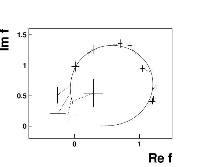
A more delicate check is to break the mass range from 1315 to 1675 MeV into 30 MeV bins and optimise the $a_{0}(1450)$ signal in each bin. The result is compared with the Argand diagram of $a_{0}(1450)$ alone on Fig. 8. The individual bins follow the expected loop closely up to 1540 MeV; dotted lines show the movement of each bin from the analytic formula. Up to this mass, there is large interference between $a_{2}(1320)$ and $a_{0}(1450)$, providing strong constraints on its phase variation with mass. Above this, three of the four remaining points show a rather large scatter. Above 1560, the effect of $a_{2}(1700)$ becomes more important than that of $a_{2}(1320)$. Final fits use Crystal Barrel parameters for $a_{2}(1700)$: $M=1660$ MeV, $\Gamma=280$ MeV [26]. The main problem is that the corner of the Dalitz plot above $m_{\eta\pi}=1560$ MeV is a cramped area in which to separate spin zero components from spin 2. The $a_{2}(1700)$ has significant contributions from all three initial states ${}^{1}S_{0}$, ${}^{3}P_{1}$ and ${}^{3}P_{2}$. These allow it to simulate a spin 0 contribution to some extent, despite the existence of the data in gas which help determine P-state contributions. The most likely explanation of the discrepancies above 1560 MeV is a poor separation between $a_{2}(1700)$ and $a_{0}(1450)$.

Finding the pole position of $a_{0}(1450)$ requires parametrisations of $a_{0}\sigma$ and $\rho\omega$ phase space and the dispersive term in the Breit-Wigner denominator. This has been done with three alternative parametrisations for each of the three terms. Formulae are chosen with good convergence properties for complex $s$, i.e. powers of $s$ confined to the denominators of the formulae. All combinations of the formulae agree within $\sim 3$ MeV for both real and imaginary parts of the pole, showing that systematic errors for the extrapolation are well under control. The pole position is $1432-i98$ MeV; the main systematic errors arise from the mean mass and width of the peak.

Fig. 9 shows as dashed curves the intensities of $a_{0}(1450)\to a_{0}(980)\sigma$ and $\omega\rho$ as they appear in production from $\bar{p}p$. The $a_{0}(980)\sigma$ decay peaks at 1458 MeV and the $\omega\rho$ decay peaks at 1476 MeV. Curves are normalised to 1 at their peaks. Full curves show the peaks for an isolated resonance without the limitation of $\bar{p}p$ phase space for production. The $a_{0}(980)\sigma$ peak is then at 1467 MeV and the $\omega\rho$ peak at 1485 MeV.

Table 2 collects results for $a_{0}(1450)$ from the final fit. At this point, it is necessary to present a more convenient formula for $a_{0}(1450)$ than Eq. (9), and the rationale behind it.

The basic points spring from the fact that there is a pole at $1432-i98$ MeV. If one knew in advance how parameters vary between the pole and the physical region, it would be best to write the formula directly in terms of the pole and its residues, which express its coupling to every channel. That is not the case, so the closest approach is to write the formula in terms of the nearby peak mass, $m_{p}=1448$ MeV and widths to each channel at this mass, together with their $s$-dependence:

This form is close to that for a Breit-Wigner resonance of constant width and is closely related to observed branching ratios between channels.

The branching fractions for an isolated resonance are given by integrals of the form

If $\rho_{j}$, hence $\Gamma_{j}(s)$, were to vary linearly with $s$, the variation of branching fractions would cancel between upper and lower halves of the peak. It turns out that this cancellation works fairly well. This form of parametrisation gives a clear insight into the way the fit responds to each parameter.

However, one important point emerges. The sum of the widths at the peak comes to 345 MeV, considerably larger than the observed full width of the peak, 192 MeV. The reasons for this are straightforward. On the lower side of the peak, $\Gamma(a_{0}(980)\sigma)$ and $\Gamma(\omega\rho)$ are small, and the amplitude falls rapidly because the remaining width to $\eta\pi$, $KK$ and $\eta^{\prime}\pi$ is small. On the upper side of the peak, $\Gamma(a_{0}(980)\sigma)$ and $\Gamma(\omega\rho)$ rapidly become large and dominate the denominator, cutting off the line-shape $1/|D(s)|^{2}$ quickly. The line-shape of $a_{0}(980)$ in Fig. 6(b) serves as a second example. The upper part of the peak is attenuated rapidly by $\Gamma_{KK}(s)$. The lower part is not far from a Breit-Wigner resonance of constant width.

The branching ratio $\Gamma(a_{0}(980)\sigma)/\Gamma(\eta\pi)$ is obtained from the combined fit. It is consistent with the magnitude of the $a_{0}(1450)$ signal fitted to $\eta\pi^{+}\pi^{-}\pi^{+}\pi^{-}$ data in Ref. [9] and with the upper limit of 4.3 established there for this ratio. The Table uses branching ratios to $\omega\rho$ from the combined fit to $\omega\pi^{+}\pi^{-}\pi^{0}$ data, discussed in detail in subsection 3.9. The Table quotes in lines 12 and 13 the ratio of branching fractions $BR(\omega\rho)/BR(\eta\pi)$ and $BR(a_{0}(980)\sigma)/BR(\eta\pi)$ as they appear in $\bar{p}p$ annihilation. These values are better defined than those for an isolated resonance because of uncertainty about its high mass tail, see Fig. 9. Note that $BR(\omega\rho)/BR(\eta\pi)$ is 7.6 in Table 2, rather smaller than the ratio $\Gamma(\omega\rho)/\Gamma(\eta\pi)=9.2$ at the peak of $a_{0}(1450)$. This is because the $\omega\rho$ signal in $\bar{p}p\to a_{0}(1450)\pi$ is inhibited at high mass by the available phase space, as illustrated in Fig. 9(b) by the dashed curve. For an isolated resonance, the $\omega\rho$ branching fraction is close to 9.2, but with an unknown error depending on form factors.

In Table 2, the first errors are statistical and the second systematic. Strong contributions to systematic errors arise from uncertainties in branching fractions for $\bar{p}p\to\eta\pi^{0}\pi^{0}$ $(\pm 5.0\%$) and $\omega\pi^{+}\pi^{-}\pi^{0}$ $(\pm 7.9\%)$. However, the largest error arises from the fact that interferences within one set of data lead to a branching fraction $\propto|\sum_{i}\Lambda_{i}f_{i}|^{2}$, rather than $\sum_{i}|\Lambda_{i}f_{i}|^{2}$. Here, the sum is over resonances, $\Lambda_{i}$ are coupling constants and $f_{i}$ are amplitudes for each resonance. The second of these quantities is derived from $\Lambda$ parameters fitted to the first, as explained above in subsection 3.5.

There is a potentially large error from the interference between the two components making up the $\pi\pi$ S-wave: the $\sigma$ pole term and the elastic component. Fortunately, the $\eta\pi^{0}\pi^{0}$ data determine both relative magnitudes and phases of these two contributions quite well. However, it is necessary to add a systematic error to cover the change to the fit if a further term is added to the parametrisation of the $\pi\pi$ S-wave. Here, it is chosen to be the elastic amplitude multiplied by $s$. There is a further small contribution to systematic errors from perturbations when small components are dropped from the fits, e.g. the weak $\pi_{1}(1400)$ contributions in both ${}^{1}S_{0}$ and ${}^{3}P_{1}$ annihilation. Finally, in view of the scatter of the last 4 points of Fig. 8 above 1540 MeV, a systematic error is included from changes in the fit if $a_{0}(1450)$ is fitted to $\eta\pi^{0}\pi^{0}$ data only up to 1540 MeV.

Table 2 includes systematic errors in fitting $\omega\pi^{+}\pi^{-}\pi^{0}$ data. The evaluation of systematic errors for these data follows the same procedure as for $\eta\pi^{0}\pi^{0}$. The final systematic errors are added in quadrature. It is not correct to add them linearly, as is sometimes done. The derivation of the Gaussian error distribution depends on the convolution of many box-shaped distributions.

The Obelix group has published two claims to observe an $a_{0}$ decaying to $\eta\pi$ in the mass range 1290-1313 MeV [27] [28]. Such a resonance should be very conspicuous in Crystal Barrel data through distinctive interference with $a_{2}(1320)$. The fits reported here have been repeated (i) using an $a_{0}$ in this mass range without $a_{0}(1450)$ and (ii) together with $a_{0}(1450)$. When $a_{0}(1450)$ is removed from the fit, $\chi^{2}$ (scaled to allow for the mean $\chi^{2}$ of 2.9 per bin) is worse by 528 for a reduction of six fitting parameters. This is an 18 standard deviation signal. If its mass and width are moved down to the mass range 1200-1340 MeV with a width $\leq 120$ MeV, there is no optimum. Instead the fit moves in a few iterations towards parameters of $a_{0}(1450)$, whatever line-shape is used for $a_{0}(1450)$. If an extra $a_{0}$ is added in the mass range 1280-1340 MeV, there is only a small improvement in $\chi^{2}$ and again no optimum for parameters in the range claimed by Obelix. The narrow width they claim $\sim 80$ MeV is similar to that of $a_{2}(1320)$. It appears likely that their signal was confused with P-state annihilation to $a_{2}(1320)$. The P-state annihilation is precisely identified in present work from data in hydrogen gas.

References

- [1] Particle Data Group, J. Phys. G 33 1 (2006).
- [2] C. Amsler et al., Phys. Lett. B 333 277 (1994).
- [3] D.V. Bugg, V.V. Anisovich, A. Sarantsev and B.S. Zou, Phys. Rev. B 50 4412 (1994).
- [4] C. Amsler et al., Phys. Lett. B 355 425 (1995).
- [5] A. Abele et al., Nucl.Phys. A 609 562 (1996); Erratum: Nucl. Phys. A 625 899 (1997).
- [6] C.A. Baker et al., Phys. Lett. B353 140 (2003).
- [7] A. Abele et al., Phys. Rev. D 57 3860 (1998).
- [8] A. Abele et al., Nucl.Phys. B 404 179 (1997).
- [9] A.V. Anisovich et al., Nucl. Phys. A 690 567 (2001).
- [10] D.V. Bugg, J. Phys. G35 075005 (2008).
- [11] V. Nikolaenko for the VES collaboration, Meson08 conference, Krakow (June 6-10) 2008.
- [12] D.V. Bugg, Eur. Phys. J C 52 55 (2007).
- [13] C. Amsler et al., Nucl. Phys. A 720 357 (2003).
- [14] A. Abele et al., Phys. Lett. B 423 175 (1998).
- [15] C. Amsler et al., Z. Phys. C 58 175 (1993).
- [16] M. Abklikim et al., Phys. Lett. B 603 138 (2004).
- [17] I. Caprini, G. Colangelo and H. Leutwyler, Phys. Rev. Lett. 96 032001 (2006).
- [18] K.M. Watson, Phys. Rev. 88 1163 (1952).
- [19] D.V. Bugg, Eur. Phys. J C 54 73 (2008).
- [20] D.V. Bugg, J. Phys. G 34 151 (2007).
- [21] Yu. A. Simonov and A.I. Veselov arXiv: hep-ph/ 0804.4635.
- [22] M. Ablikim et al., Phys. Lett. B 607 243 (2005).
- [23] R. Escribano and J. Nadal, arXiv: hep-ph/0703187.
- [24] C.E. Thomas, JHEP 10 026 (2007).
- [25] R. Escribano, arXiv: hep-ph/0802.3909.
- [26] A. Abele et al., Eur. Phys. J C 8 67 (1999).
- [27] A. Bertin et al., (Obelix Collaboration) Phys. Lett. B 434 180 (1998).
- [28] M. Bargiotti et al., (Obelix Collaboration) Eur. Phys. J C 26 371 (2003).
- [29] A. Anisovich et al., Phys. Lett. B 485 341 (2000).
- [30] F. Meyer-Wildhagen, Ph. D. thesis, University of Munich, (2004).
- [31] D.V. Amelin et al. (VES Collaboration), Yad. Fis. 62 1021 (1999), translated in Phys. At. Nuclei 62 (1999) 445.
- [32] D. Aston et al. (LASS Collaboration), Nucl. Phys. B 296 493 (1988).
- [33] D.V. Bugg, Phys. Lett. B 632 471 (2006).
- [34] D.V. Bugg, Eur. Phys. J A 25 107 (2005).
- [35] E.M. Aitala et al. (E791 Collaboration), Phys. Rev. D 73 032004 (2006).
- [36] B. Aubert et al. (Babar Collaboration), arXiV: hep-ex/0710.4451.
- [37] A. Aloisio et al. (Kloe Collaboration), Phys. Lett. B 536 209 (2002).
- [38] F. Ambrosino et al. (Kloe Collaboration), arXiv: hep-ex/0707.4609 (2007).
- [39] N.N. Achasov and V.N. Ivanchenko, Nucl. Phys. B 315 465 (1989).
- [40] D.V. Bugg, Eur. Phys. J C 47 45 (2000).
- [41] D. Black, A.H. Fariborz and J. Schechter, Phys. Rev. D 61 074001 (2000).