Time-delay interferometry and the relativistic treatment of LISA optical links
Abstract
LISA is a joint space mission of the ESA and NASA for detecting low frequency gravitational radiation in the band Hz. In order to attain the requisite sensitivity for LISA, the laser frequency noise must be suppressed below the other secondary noises such as the optical path noise, acceleration noise etc. This is achieved because of the redundancy in the data, more specifically, by combining six appropriately time-delayed data streams containing fractional Doppler shifts - time delay interferometry (TDI). The orbits of the spacecraft are computed in the gravitational field of the Sun and Earth in the Newtonian framework, while the optical links are treated fully general relativistically and thus, effects such as the Sagnac, Shapiro delay, etc. are automatically incorporated. We show that in the model of LISA that we consider here, there are symmetries inherent in the physics, which may be used effectively to suppress the residual laser frequency noise and simplify the algebraic approach to TDI.
pacs
95.55.Ym, 04.80.Nn, 07.60.Ly1 Introduction
LISA - Laser Interferometric Space Antenna - is a proposed mission which will use coherent laser beams exchanged between three identical spacecraft forming a giant (almost) equilateral triangle of side kilometres to observe and detect low frequency cosmic GW [1].
In ground based detectors the arms are as symmetrical as possible so that the laser light experiences nearly identical delay in each arm of the interferometer which reduces the laser frequency/phase noise at the photodetector. However, in LISA, the lack of symmetry will be much larger than in terrestrial instruments. Laser frequency noise dominates the other secondary noises, such as optical path noise, acceleration noise by 7 or 8 orders of magnitude, and must be removed if LISA is to achieve the required sensitivity of , where is the metric perturbation caused by a gravitational wave. In LISA, six data streams arise from the exchange of laser beams between the three spacecraft approximately 5 million km apart. These six streams produce redundancy in the data which can be used to suppress the laser frequency noise by the technique called time-delay interferometry (TDI) in which the six data streams are combined with appropriate time-delays [2].
This work was put on a sound mathematical footing by showing that the data combinations constituted an algebraic structure; the data combinations cancelling laser frequency noise formed the module of syzygies over the polynomial ring of time-delay operators [3]. The module was obtained - that is its generators were obtained - for the simple case of stationary LISA in flat spacetime. These were the so-called first generation TDI. However, LISA spacecraft execute a rotational motion, the arm-lengths change with time and the background spacetime is curved, all of which affect the optical links and the time-delays. The rotation gives rise to the Sagnac effect which implies that the up-down optical links are unequal, the arm-lengths or the time-delays change with time - flexing of arms. These effects cannot be ignored if the laser frequency noise is to be effectively cancelled.
In this paper, we compute the orbits of spacecraft in the Newtonian framework where the Earth’s gravitational field is also taken into account. The base orbits we take to be Keplerian in the gravitational field of the Sun only. On these base orbits, we linearly superpose the perturbative effect of the Earth’s gravitational field. We choose the Earth over Jupiter because (i) the Earth perturbs the Keplerian orbit in resonance, resulting in a secular growth of the perturbations and, (ii) Jupiter’s effect is less than 10 of that of the Earth’s on the flexing and hence not dominant. The perturbative analysis is carried out within the Clohessy-Wiltshire (CW) [4] framework. Further, an extension of the previous algebraic approach is proposed for the general problem in which the time-delay operators in general do not commute; this leads to the second generation TDI and imperfect cancellation of laser frequency noise. However, we show that there are symmetries in the physical model which can simplify to some extent the totally non-commutative problem. These computations will be useful in the development of a LISA simulators, the LISACode for instance [5].
2 The spacecraft orbits in the Sun’s and Earth’s field
The Keplerian orbits, the orbital motion in the gravitational field of the Sun only are chosen so that the peak to peak variation in armlengths is the least km, see [6]. We summarise the results of paper [6] below. We choose the Sun as the origin with Cartesian coordinates as follows: The ecliptic plane is the plane and we consider a circular reference orbit of radius 1 A. U. centred at the Sun. Let where and km is a constant representing the nominal distance between two spacecraft of the LISA configuration. We choose the tilt of the plane of the LISA triangle to be which has been shown to yield minimum flexing of the arms. We choose spacecraft 1 to be at its lowest point (maximum negative Z) at . This means that at this point, and . The orbit of the first spacecraft is an ellipse with inclination angle , eccentricity and satisfying the above initial condition.
From the geometry, and are obtained as functions of ,
| (1) |
The equations for the orbit of spacecraft 1 are given by:
| (2) |
The eccentric anomaly is implicitly given in terms of by,
| (3) |
where is the time and is the average angular velocity and the initial phase. The orbits of the spacecraft 2 and 3 are obtained by rotating the orbit of spacecraft 1 by and about the axis; the phases , however, must be adjusted so that the spacecraft are at a distance from each other. The orbital equations of spacecraft are:
| (4) |
where , with the caveat that the is replaced by the phases , where they are implicitly given by,
| (5) |
These are the exact (Keplerian) expressions for the orbits of the three spacecraft in the Sun’s field.
The Earth’s field is now included perturbatively using the CW framework. The CW frame is chosen as follows: We take the reference particle to be orbiting in a circle of radius with constant Keplerian angular velocity . Then the transformation to the CW frame from the barycentric frame is given by,
| (6) |
The direction is normal and coplanar with the reference orbit, the direction is tangential and comoving, and the direction is chosen orthogonal to the orbital plane. Linearised dynamical equations for test-particles in the neighbourhood of the reference particle are easily obtained. Since the frame is noninertial, Coriolis and centrifugal forces appear in addition to the tidal forces. With the help of the CW formalism, it is easy to see that to the first order in (or equivalently ) there exist configurations of spacecraft so that the mutual distances between them remain constant in time. The flexing appears only when we consider second and higher order terms in . In fact in [6] we have shown that the second order terms describe the flexing of LISA’s arms quite accurately as compared to the exact Keplerian orbits.
The CW equations for a test particle are given by:
| (7) |
We choose those solutions of Eq.(7) which form an equilateral triangular configuration of side (such solutions exist). For the th spacecraft we have the following position coordinates:
| (8) |
where . Also at the initial phase of the configuration is described through . In this solution, any pair of spacecraft maintain the constant distance between each other.
LISA follows the Earth behind. We consider the model where the centre of the Earth leads the origin of the CW frame by - thus in our model, the ‘Earth’ or the centre of force representing the Earth, follows the circular reference orbit of radius 1 A. U. Also the Earth is at a fixed position vector in the CW frame. We find that km, km and . The acceleration field due to the Earth at any point (in particular at any spacecraft) in the CW frame is given by:
| (9) |
where kg is the mass of the Earth and Newton’s gravitational constant.
In order to write the CW equations in a convenient form we first define the small parameter in terms of the quantity , where is the distance of the Earth from the origin of the CW frame; km which is more than 50 million km. So when deriving the forcing term we make the aprroximation , that is, we neglect compared to . It will turn out that the flexing due to the Earth is small so that this approximation is not unjustified. We define which is the just the ratio of the tidal forces due to the Earth and the Sun. The CW equations including the Earth’s field take the form:
| (10) |
Note that the compounded flexing due to the combined field of Earth and Sun is a nonlinear problem; it is infact a three body problem. We however solve this problem approximately. Assuming that both effects are small we may linearly add the flexing vectors due to the Sun and Earth; that is, add the perturbative solutions obtained from Eqs.(7) and (10); the nonlinearities appear at higher orders in and . These would modify the flexing but we may neglect this effect because of the smallness. We find that the flexing produced by the Earth is of the order of 1 or 2 m/sec upto the third year, just about 40 of that due to the Sun. But, as shown in [6] the flexing produced by the Sun’s octupole field is nearly exact to that produced by the Keplerian orbits. Thus we may do better by just adding the flexing vector produced by the Earth to the Keplerian orbit of the relevant spacecraft.
We then seek perturbative solutions to Eq. (10) to the first order in . We write, where are solutions at the zeroth order given by Eq.(8). We put (or equivalently include it in ) in these solutions for simplifying the algebra.
With the initial conditions: at , we have the results:
| (11) | |||||
where,
| (12) |
The equation can be exactly integrated and used directly to obtain the flexing. However, we can also expand this solution to the first order in and the result is:
| (13) |
As argued before, we add the perturbation given by to the Keplerian orbit of each spacecraft. Next we compute the optical links.
3 The six optical links
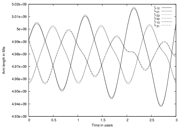
The time-delay that is required for the TDI operators needs to be known very accurately - at least to 1 part in , that is, to about few metres - for the laser frequency noise to be suppressed. In order to guarantee such level of accuracy, we numerically compute the optical links or the time-delay. This approach is guaranteed to give the desired accuracy or even better accuracy than what is required. We numerically integrate the null geodesics followed by the laser ray emitted by one spacecraft and received by the other. This computation is performed in the barycentric frame, and taking into account the fact that the spacetime is curved by the Sun’s mass only (the Earth’s contribution is about 5 orders of magnitude less). The computation here is further complicated by the fact that the spacecraft are moving in this frame of reference and the photon emitted from one spacecraft must be received by the other spacecraft. We use the Runga-Kutta numerical scheme to integrate the differential equations describing the null geodesics. But since the end point of the photon trajectory is not known apriori, an iterative scheme must be devised for adjusting the parameters of the null geodesic, in order that the worldlines of the photon and the receiving spacecraft intersect. We have devised such a scheme based on the difference vector between the photon position vector and receiving spacecraft position vector. The six optical links have thus been numerically computed with sufficient accuracy required for TDI. The code gives results accurate to better than 10 metres - most of the time better than metres - except in a window of about half an hour when the error exceeds this value and becomes unacceptably large. We display the results in Figures 1 and 2 for . More details may be found in [8].
Figure 1 shows all the six optical links in the combined field of the Sun and Earth.
We also need to estimate the variation in armlength which is important for the TDI analysis to follow. Figure 2 shows the rate of change of the six optical links as a function of time over a period of three years.
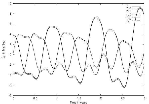
We find that in the optimised model of LISA configuration, this rate of change is less than 4 m/sec. if we just consider the Sun’s field. Including the Earth’s field the flexing still remains m/sec in the first two years and increases to m/sec in the third year. Earlier estimates were m/sec. These numerical estimates are most crucial for their effect on residual laser frequency noise in the TDI.
4 Time-delay interferometry
In order to cancel the laser frequency noise, time-delayed data streams are added together in which an appropriate set of time-delays are chosen. In general the time-delays are multiples of the photon transit time between pairs of spacecraft. In [3] a scheme based on modules over commutative rings was given where the module of data combinations cancelling the laser noise was constructed. This fully cancels the laser frequency noise for stationary LISA. There are only three delay operators corresponding to the three armlengths and the time-delay operators commute. This scheme can be straight forwardly extended to moving LISA [7], where, now because of Sagnac effect, the up and down optical links have different armlengths but the armlengths are still constant in time. In this case, there are six delay operators corresponding to the six optical links and they commute. These are the modified but still first generation TDI. However, for LISA the armlengths do change with time - flexing of the arms - and the first generation TDI modified or otherwise do not cancel of the laser frequency noise sufficiently.
4.1 Equations for the polynomial vector cancelling laser frequency noise
We follow the notation and conventions of [7] and [3] which are the simplest for our purpose. The six links are denoted by . The time-delay operator for the link from S/C 1 to S/C 2 or is denoted by in [7] and so on in a cyclic fashion. The delay operators in the other sense are denoted by ; the link from by and similarly the links are defined through cyclic permutation.
Let represent the laser frequency noise in S/C . Let be the delay operator corresponding to the variable armlength , i.e. . Then we have,
| (14) |
The other links in terms of are obtained by cyclic permutations. Also in the we have not included contributions from the secondary noises, gravitational wave signal etc. since here our aim is to deal with laser frequency noise only. Any observable is written as:
| (15) |
where are polynomials in the variables . Thus is specified by giving the six tuple polynomial vector . Writing out the in terms of the laser noises , and in order that the laser frequency noise cancel for arbitrary , the polynomials must satisfy the equations:
| (16) |
The solutions to these equations as realised in earlier works are important, because they consist of polynomials with lowest possible degrees and thus are simple. Since these are linear equations they define a homomorphism of modules and the solutions themselves form a module - the module of syzygies over the polynomial ring , where is the field of rational numbers and play the role of indeterminates. In general, the variables (operators) do not commute and hence the order of the variables is important. However, if we assume in a simple model that the arms do not flex, then the operators commute, and the generators of the module have been found via Gröbner basis methods [3, 7].
However, when the arms flex, the operators no longer commute. If we operate on with operators and in different orders, it is easily seen that . A combinatorial approach has been adopted in [9] to deal with the totally non-commutative case. However, our aim here is to estimate the level of the non-commutativity of these operators in the context of our LISA model and use the symmetries to simplify the algebraic approach.
4.2 The algebraic approach and symmetries
The level of non-commutativity can be found by computing commutators which occur in several of the well known TDI observables like the Michelson, Sagnac etc. We find that given our model of LISA, we require to go only upto the first order in ; we find for our model metres/sec2 and thus even if one considers say 6 successive optical paths, that is, about seconds of light travel time, metres. This is well below few metres and thus can be neglected in the residual laser noise computation. Moreover, terms (and higher order) can be dropped since they are of the order of (they come with a factor ) which is much smaller than 1 part in . The calculations which follow neglect these terms.
Applying the operators twice in succession and dropping higher order terms as explained above,
| (17) | |||||
The above formula can be easily generalised by induction to operators.
We now turn to the commutators of the operators. The term in cancels out; only the term remains. We list below a few of the commutators:
| (18) | |||||
| (19) |
We observe the following approximate symmetries in our model:
| (20) |
which also implies (this combination occurs in the Sagnac observables),
| (21) |
Infact in our model, m/sec and m/sec upto the first three years in our model. The same is essentially true for the pairs of links and . Thus these pairs of operators essentially commute. Thus, we are not dealing with a set of totally non-commuting variables, but with an intermediate case.
In addition to these approximate symmetries there are other commutators which vanish ‘identically’ (after dropping terms in and and higher order). It can be easily verified that commutators of the form, vanish identically, when the are permutation of the operators , and the for a given represents one of the delay operators . Thus the original non-commutative ring can be quotiented by the ideal which is generated by the vanishing and approximately vanishing commutators: . The quotient ring is clearly much smaller and simpler and the solution to Eq. (16) is sought for polynomials in this quotient ring. The solution set of polynomial vectors still form a module over . The future goal is to ‘construct’ this module.
4.3 Residual laser frequency noise in the Sagnac observable and symmetries
By the time LISA flies the expectations are for the laser frequency noise estimate to reduce to say . If we divide this number by the laser frequency Hz, we obtain the noise estimate in the fractional Doppler shift with the power spectral density (PSD):
| (22) |
where is the Fourier transform of . Then by differentiating , the PSD of the random variable is just Hz.
The modified Sagnac first generation TDI observable is given by the polynomial vector in the form by:
| (23) |
where and . If the variables commute then the laser frequency noise is fully cancelled. However, if they do not commute, there is a residual term. It can be computed as:
| (24) |
We find that and and so by Eq. (19):
| (25) |
and thus . Because the vary during the course of an year the also varies during the year and so also the amplitude of the random variable . Thus the PSD of is:
| (26) |
This noise must be compared with the secondary noise [1]. However, because we are considering the modified TDI Eq. (23), there are extra factors and which do not appear in the corresponding first generation TDI. These factors introduce an additional multiplicative factor, namely, in the secondary noise PSD which leaves the SNR unchanged but must be considered when it is compared with the residual laser frequency noise given in Eq. (26). Thus,
| (27) |
where and . In the Figure 3 we plot and at three epochs an year apart.
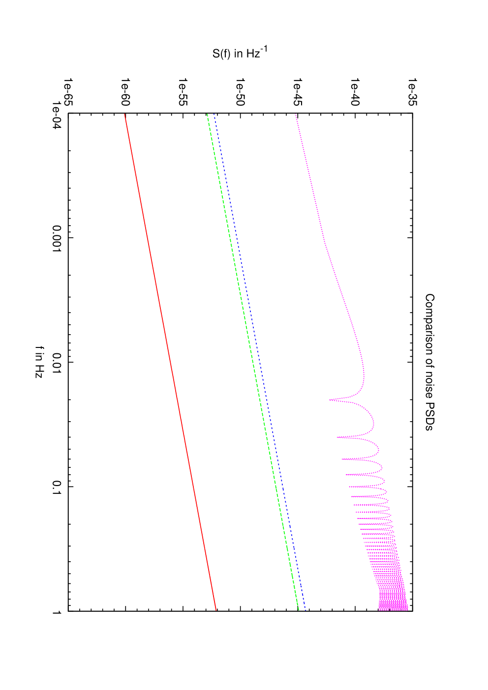
We see that, clearly the residual laser frequency noise is few orders of magnitude below the secondary noises. Since the other Sagnac variables and are obtained by cyclic permutations of the spacecraft, the residual laser noise is similarly suppressed in them. The basic reason for this remarkable cancellation is the symmetry inherent in the physics. Note that and hence is an element of the module we are seeking.
5 Concluding remarks
We have computed in the Newtonian framework the spacecraft orbits in the combined field of the Sun and Earth and from this deduced the flexing of the arms of LISA by choosing the model which gave minimum flexing when only the Sun’s field was taken into account. Now the flexing is no more periodic as was the case when only the Sun’s field was considered. We have ignored the effect of Jupiter because we believe this effect to be not so dominant as that of the Earth. Writing the tidal parameter for Jupiter, , similar to of Earth, where, kg is the mass of Jupiter and , the distance from LISA to Jupiter, which we take on the average to be A. U., we find . Moreover, Jupiter has its own periodicity pertaining to its orbit and therefore will not be in resonance as was the case with the Earth, and thus there will be no secular effect. Thus we do not expect the effect of Jupiter on flexing to dominate. Note that these results are valid so long as we can neglect the nonlinearities arising from higher order terms in and .
We have computed the residual laser frequency noise in one of the important TDI variables, namely, the Sagnac. The residual noise is satisfactorily suppressed because of the symmetry. In other variables such as the Michelson this is not true and higher degree polynomials will be required. The algebraic approach outlined above seems promising.
Our model of LISA is optimal (minimal flexing of arms) only in the Sun’s field. Clearly this opens up the question of seeking an optimal model for the LISA configuration in the field of the Sun, Earth, Jupiter and other planets which will minimise the flexing of the arms and therefore the residual laser frequency noise in the modified first generation TDI. We finally remark that our computations here may be useful in the development of a LISA simulator.
References
- [1] P. Bender et al. "LISA: A Cornerstone Mission for the Observation of Gravitational Waves", System and Technology Study Report ESA-SCI(2000) 11, 2000.
- [2] J. W. Armstrong, lrr-2006-1 : http://relativity.livingreviews.org/Articles/lrr-2008-2.
- [3] S. V. Dhurandhar, K. Rajesh Nayak, J-Y. Vinet, Phys. Rev, D 65 , 102002(2002).
- [4]
W. H. Clohessy and R. S. Wiltshire, Journal of Aerospace Sciences, 653 - 658 (1960);
D. A. Vallado, Foundations of Astrodynamics and Applications, 2nd edition 2001, Microcosm Press Kluwer;
also in S. Nerem, http://ccar.colorado.edu/asen5050/lecture12.pdf(2003). - [5] A. Petiteau, G. Auger, H. Halloin, O. Jeannin, E. Pagnol, S. Pireaux, T. Regimbau and J-Y. Vinet, Phys. Rev. D 77, 023002 (2008).
- [6] S. V. Dhurandhar, K. R. Nayak, S. Koshti and J-Y. Vinet, Class. Quantum Grav., 22, 481 (2005); R. Nayak, S. Koshti, S. V. Dhurandhar and J-Y. Vinet, Class. Quantum Grav., 22, 1763 (2006).
- [7] K. R. Nayak and J-Y Vinet, Phys. Rev. D 70, 102003 (2004).
- [8] S. V. Dhurandhar, J-Y. Vinet and K. R. Nayak, submitted to CQG, gr-qc 0805.4314, (2008).
- [9] M. Vallisneri, Phys. Rev. D 72, 04003 (2005).