跳到论文正文
W Papers独立论文阅读器 arXiv:0808.2548 论文正文 计算阅读时间 · 0%
引用这篇论文根据当前论文元数据生成,正式投稿前建议核对。


License: arXiv.org perpetual non-exclusive license
arXiv:0808.2548v2 [cs.IT] 28 Jul 2009

Negative β\beta-encoder

Tohru Kohda    Satoshi Hironaka    and Kazuyuki Aihara ††thanks: T. Kohda and S. Hironaka are with the Department of Computer Science and Communication Engineering, Kyushu University Motooka 744, Nishi-ku, Fukuoka-city 819-0395, Japan, Phone +81-92-802-3623, Fax +81-92-802-3627, (email: kohda@csce.kyushu-u.ac.jp)††thanks: K. Aihara is with the Department of Mathematical Engineering and Information Physics, Faculty of Engineering, Tokyo University and Aihara Complexity Modeling Project, ERATO, JST
Abstract

A new class of analog-to-digital (A/D) and digital-to-analog (D/A) converters using a flaky quantiser, called the β\beta-encoder, has been shown to have exponential bit rate accuracy while possessing a self-correction property for fluctuations of the amplifier factor β\beta and the quantiser threshold ν\nu. The probabilistic behavior of such a flaky quantiser is explained as the deterministic dynamics of the multi-valued Rényi map. That is, a sample xx is always confined to a contracted subinterval while successive approximations of xx are performed using β\beta-expansion even if ν\nu may vary at each iteration. This viewpoint enables us to get the decoded sample, which is equal to the midpoint of the subinterval, and its associated characteristic equation for recovering β\beta which improves the quantisation error by more than 3​dB3\mbox{dB} when β>1.5\beta>1.5. The invariant subinterval under the Rényi map shows that ν\nu should be set to around the midpoint of its associated greedy and lazy values. Furthermore, a new A/D converter is introduced called the negative β\beta-encoder, which further improves the quantisation error of the β\beta-encoder. A two-state Markov chain describing the β\beta-encoder suggests that a negative eigenvalue of its associated transition probability matrix reduces the quantisation error.

Index Terms: 
Analog-to-digital (A/D) conversion, flaky quantiser, β\beta-expansion, β\beta-encoder, chaotic dynamics, PCM, Σ​Δ\Sigma\Delta modulation, Markov chain.

I Introduction

SAMPLING and quantisation are necessary in almost all signal processing. The combined operations are called analog-to-digital (A/D) conversion. Since A/D converters are analog circuits, they have the fundamental problem that instability of the circuit elements degrades the A/D conversion. There are a number of possible remedies to cope with this problem.

The standard sampling theorem states that if a band-limited signal f⁡(t)f(t) is sampled at rates far above the Nyquist rate, called oversampling, then it can be reconstructed from its samples, denoted by {f⁡(nM)}n∈𝒵\{f(\dfrac{n}{M})\}_{n\in{\cal Z}} (with M>1M>1), by the use of the following formula with an appropriate function φ⁡(t)\varphi(t),  [1, 2, 3]

f⁡(t)=1M​∑n∈𝒵f⁡(nM)​φ​(t−nM).f(t)=\dfrac{1}{M}\sum_{n\in{\cal Z}}f(\dfrac{n}{M})\varphi(t-\dfrac{n}{M}). (1)

The above formula does not result in a loss of information. However, since the amplitudes of the samples are continuous variables, each sample is quantised according to amplitude into a finite number of levels. This quantisation process necessarily introduces some distortion into the output. The magnitude of this type of distortion depends on the method by which the quantisation is performed.

Various kinds of A/D and digital-to-analog (D/A) conversions have been proposed. Related topics include one-bit coding through over-sampled data [4] and high-quality AD conversions using a coarse quantiser together with feedback [5], the concept of “democracy” [6], in which the individual bits in a coarsely quantised representation of a signal are all given “equal weight” in the approximation to the original signal, a pipelined AD converter [7], and a single-bit oversampled AD conversion using irregularly spaced samples [3].

Given a bandlimited function ff, the LL-bit pulse code modulation (PCM) [8] simply uses each sample value f⁡(n/M)f(n/M) with LL bits: one bit for its sign, followed by the first L−1L-1 bits of the binary expansion of f⁡(n/M)f(n/M). It is possible to show that for a bandlimited signal, this algorithm achieves precision of order O⁡(2−L)O(2^{-L}). On the other hand, Σ​Δ\Sigma\Delta modulation  [1, 2, 9, 10, 11], another commonly implemented quantisation algorithm for a bandlimited function, achieves precision that decays like an inverse polynomial in the bit budget LL. For example, a kkth-order Σ​Δ\Sigma\Delta scheme produces an approximation where the distortion is of the order O⁡(L−k)O(L^{-k}). Although PCM is superior to Σ​Δ\Sigma\Delta modulation in its level of distortion for a given bit budget, Σ​Δ\Sigma\Delta modulation has practical features for analog circuit implementation. One of the key features is a ceratain self-correction property for quantiser threshold errors (bias) that is not shared by PCM. This is one of several reasons why Σ​Δ\Sigma\Delta modulation is preferred for A/D conversion in practice.

In 2002, Daubechies et al. [12] introduced a new architecture for A/D converters called the β\beta-encoder and showed the interesting result that it has exponential accuracy even if the β\beta-encoder is iterated at each step in successive approximation of each sample using an imprecise quantiser with a quantisation error and an offset parameter. Furthermore, in a subsequent paper [13], they introduced a “flaky” version of an imperfect quantiser, defined as

Q[ν0,ν1]f​(z)={0,if​z≤ν0,1,if​z≥ν1,0​or​ 1,if​z∈(ν0,ν1),Q^{f}_{[\nu_{0},\nu_{1}]}(z)=\left\{\begin{array}[]{lcr}0,&\mbox{if}\,z\leq\nu_{0},\\ 1,&\mbox{if}\,z\geq\nu_{1},\\ 0\,\mbox{or}\,1,&\mbox{if}\,z\in(\nu_{0},\nu_{1}),\end{array}\right. (2)

where 1≤ν0<ν1≤(β−1)−11\leq\nu_{0}<\nu_{1}\leq(\beta-1)^{-1} and made the remarkable observation that ‘‘greedy” and ‘‘lazy” as well as ‘‘cautious”11 1 Intermediate expansions [14] between the greedy and lazy expansions are called “cautious” by Daubechies et al. [13]. expansions in the β\beta-encoder with such a flaky quantiser exhibit exponential accuracy in the bit rate. This β\beta-encoder was a milestone in oversampled A/D and D/A conversions in the sense that it may become a good alternative to PCM. The primary reason is that the β\beta-encoder consists of an analog circuit, with an amplifier with the factor β\beta, a single-bit quantiser with the threshold ν\nu and a single feedback loop for successive LL-bit quantisation of each sample which uses the bit-budget efficiently, like PCM. The β\beta-encoder further guarantees the robustness of both β\beta and ν\nu against fluctuations like Σ​Δ\Sigma\Delta modulation. Nevertheless, it provides a simple D/A conversion using the estimated β\beta without knowing the exact value of β\beta with its offset in the A/D conversion [15].

This paper is devoted to dynamical systems theory for studying ergodic-theoretic and probabilistic properties of the β\beta-encoder as a nonlinear system with feedback. We emphasize here that the flaky quantiser QΔβf​(⋅)Q^{f}_{\Delta_{\beta}}(\cdot) is exactly realized by the multi-valued Rényi map (i.e., β\beta-transformation) [20] on the middle interval Δβ=[β−1,β−1​(β−1)−1]\Delta_{\beta}=[\beta^{-1},\beta^{-1}(\beta-1)^{-1}] so that probabilistic behavior in the “flaky region” Δβ\Delta_{\beta} is completely explained using dynamical systems theory. Our purpose is to give a “dynamical” version of Daubechies et al.’s proof for the exponential accuracy of the β\beta-encoder as follows. We can observe that a sample xx is always confined to a subinterval of the contracted interval defined in this paper while the successive approximation of xx is stably22 2 A small real-valued quantity, approximately proportional to the quantisation error, does not necessarily converge to any fixed value, e.g., 00 but may oscillate without diverging as discussed later in detail. Such a phenomenon is sometimes referred to as chaos. performed using β\beta-expansion even if ν\nu may vary at each iteration. This enables us to obtain the decoded sample easily, as it is equal to the midpoint of the subinterval, and it also yields the characteristic equation for recovering β\beta which improves the quantisation error by more than 3​dB3\mbox{dB} over Daubechies et al.’s bound when β>1.5.\beta>1.5. Furthermore, two classic β\beta-expansions, known as the greedy and lazy expansions are proven to be perfectly symmetrical in terms of their quantisation errors. The invariant subinterval of the Rényi map further suggests that ν\nu should be set to around the midpoint of its associated greedy and lazy values. This paper presents a radix expansion of a real number in a negative real base, called a negative β\beta-expansion and a negative β\beta-encoder in order to make stable analog circuit implementation easier. Finally we observe a clear difference between a sequence of independent and identically distributed (i.i.d.) binary random variables generated by PCM and a binary sequence generated by the β\beta-encoder based on the viewpoint that if the latter sequence is regarded as a 22-state Markov chain with a 2×22\times 2 transition probability matrix, then the matrix has a negative eigenvalue.

First, we survey PCM from the viewpoint of dynamical systems because it is a typical example of a nonlinear map. PCM is an A/D converter that realizes binary expansion in the analog world. The binary expansion of a given real number r∈[−1,1]r\in[-1,1] has the form

r=b0,B​∑i=1∞bi,B​2−i,r=b_{0,B}\sum^{\infty}_{i=1}b_{i,B}2^{-i}, (3)

where b0,B=b0,B​(r)∈{−1,1}b_{0,B}=b_{0,B}(r)\in\{-1,1\} is the sign bit, and bi,B=bi,B​(r)∈{0,1}​i≥1b_{i,B}=b_{i,B}(r)\in\{0,1\}\ i\geq 1 are the binary digits of |r||r|. We define the quantiser function Q1​(⋅)Q_{1}(\cdot) as

Q1​(x)={0,x<1,1,x≥1.Q_{1}(x)=\left\{\begin{array}[]{ll}0,&x<1,\\ 1,&x\geq 1.\end{array}\right. (4)

Then we have bi,Bb_{i,B} which can be computed by the following algorithm. Let u1=2​|r|u_{1}=2|r|; the first bit b1,Bb_{1,B} is then given by b1,B=Q1​(u1)b_{1,B}=Q_{1}(u_{1}). The remaining bits are determined recursively: if uiu_{i} and bi,Bb_{i,B} have been given, then we can define

ui+1=2​(ui−bi,B)u_{i+1}=2(u_{i}-b_{i,B}) (5)

and

bi+1,B=Q1​(ui+1),b_{i+1,B}=Q_{1}(u_{i+1}), (6)

respectively. Such a sequence is also obtained with the Bernoulli shift map B⁡(x)B(x) [16, 17, 18], defined by

B⁡(x)=2​x​mod​ 1={2​x,x<1/2,2​x−1,x≥1/2,B(x)=2x\ \mbox{mod}\ 1=\left\{\begin{array}[]{ll}2x,&x<1/2,\\ 2x-1,&x\geq 1/2,\\ \end{array}\right. (7)

and its associated bit sequence bi,B​(i=1,2,…)b_{i,B}(i=1,2,\ldots), defined by

bi,B={0,Bi−1​(x)<1/2,1,Bi−1​(x)≥1/2.b_{i,B}=\left\{\begin{array}[]{ll}0,&B^{i-1}(x)<1/2,\\ 1,&B^{i-1}(x)\geq 1/2.\\ \end{array}\right. (8)

Iterating B⁡(x)B(x) for x∈[0,1)x\in[0,1) gives

Bi+1(x)=2Bi(x)−bi,B,i=1,2,⋯,L∈ℕ.B^{i+1}(x)=2B^{i}(x)-b_{i,B},\,i=1,2,\cdots,L\in\mathbb{N}. (9)

Then

BL​(x)\displaystyle B^{L}(x) =\displaystyle= 2(⋯2(2x−b1,B)−b2,B⋯)−bL,B\displaystyle 2(\cdots 2(2x-b_{1,B})-b_{2,B}\cdots)-b_{L,B} (10)
=\displaystyle= 2L​x−∑i=1Lbi,B​2L−i\displaystyle 2^{L}x-\sum^{L}_{i=1}b_{i,B}2^{L-i}

or

x=∑i=1Lbi,B​2−i+2−L​BL​(x).\displaystyle x=\sum^{L}_{i=1}b_{i,B}2^{-i}+2^{-L}B^{L}(x). (11)

Hence 2−L​BL​(x)=02^{-L}B^{L}(x)=0 as L→∞L\rightarrow\infty because BL​(x)∈[0,1)B^{L}(x)\in[0,1). That is, we get the binary expansion of xx:

x=∑i=1∞bi,B​2−i.\displaystyle x=\sum^{\infty}_{i=1}b_{i,B}2^{-i}. (12)

Suppose that a threshold shift ρ\rho occurs. Let Bρ​(x)B_{\rho}(x) be the resulting map:

Bρ​(x)={2​x,x<(1+ρ)/2,2​x−1,x≥(1+ρ)/2,B_{\rho}(x)=\left\{\begin{array}[]{ll}2x,&x<(1+\rho)/2,\\ 2x-1,&x\geq(1+\rho)/2,\\ \end{array}\right. (13)

and bi,Bρ​(i=1,2,…)b_{i,B_{\rho}}(i=1,2,\ldots) its bit sequence:

bi,Bρ={0,Bρi−1​(x)<(1+ρ)/2,1,Bρi−1​(x)≥(1+ρ)/2.b_{i,B_{\rho}}=\left\{\begin{array}[]{ll}0,&B_{\rho}^{i-1}(x)<(1+\rho)/2,\\ 1,&B_{\rho}^{i-1}(x)\geq(1+\rho)/2.\\ \end{array}\right. (14)

Then we have its associated binary expansion of x, defined as

x=∑i=1Lbi,Bρ​2−i+2−L​BρL​(x).x=\sum^{L}_{i=1}b_{i,B_{\rho}}2^{-i}+2^{-L}B_{\rho}^{L}(x). (15)

When ρ>0\rho>0, we have Bρ(x):[0,1)→[0,1+ρ)B_{\rho}(x):[0,1)\rightarrow[0,1+\rho) for x∈[0,1)x\in[0,1). Iterating Bρ​(x)B_{\rho}(x) LL times gives BρL(x):[0,1)→[0,1+2L−1ρ)B^{L}_{\rho}(x):[0,1)\rightarrow[0,1+2^{L-1}\rho). Thus we have

0≤x−∑i=1Lbi,Bρ​2−i<2−L+ρ2.0\leq x-\sum^{L}_{i=1}b_{i,B_{\rho}}2^{-i}<2^{-L}+\dfrac{\rho}{2}. (16)

Conversely, suppose that ρ<0\rho<0; then we get Bρ​(x):[0,1)→[ρ,1)B_{\rho}(x):[0,1)\rightarrow[\rho,1) for x∈[0,1)x\in[0,1). Iterating Bρ​(x)B_{\rho}(x) LL times gives BρL​(x):[0,1)→[2L−1​ρ,1)B^{L}_{\rho}(x):[0,1)\rightarrow[2^{L-1}\rho,1) which implies that

ρ2≤x−∑i=1Lbi,Bρ​2−i≤0.\dfrac{\rho}{2}\leq x-\sum^{L}_{i=1}b_{i,B_{\rho}}2^{-i}\leq 0. (17)

Both (16) and (17) show that an A/D conversion does not work well because the quantisation errors don’t decay.

Refer to caption
Fig. 1: The divergence of a value xx in PCM when there is a threshold shift ρ>0\rho>0.

Figure 1 shows the divergence of a value xx in PCM when there is a threshold shift ρ>0\rho>0. Such a map must be a mapping interval into interval (or at least a mapping interval onto interval) so that the A/D conversion operates normally. Fluctuations of the threshold are inevitable because every A/D converter is implemented as an analog circuit.

However, β\beta-encoders which realize β\beta-expansion using the expansion by β∈(1,2)\beta\in(1,2) as a radix, overcome this problem.

Refer to caption
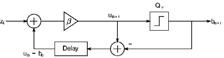
Fig. 2: A β\beta-encoder: for input z0=y∈[0,1),zi=0,i>1z_{0}=y\in[0,1),z_{i}=0,i>1, and “initial conditions” u0=0u_{0}=0 and b0,β=0b_{0,\beta}=0, the output (bi,β)i≥1(b_{i,\beta})_{i\geq 1} gives the β\beta-expansion for yy defined by the quantiser Qν=Q1(⋅/ν)Q_{\nu}=Q_{1}(\cdot/\nu), with ν∈[1,(β−1)−1]\nu\in[1,(\beta-1)^{-1}]. This provides the “greedy” and “lazy” schemes for ν=1\nu=1 and ν=(β−1)−1\nu=(\beta-1)^{-1}, respectively. The β\beta-encoder with β=2\beta=2 and ν=1\nu=1 gives PCM.

The block diagram of the β\beta-encoder is shown in Fig.2 with the amplifier β∈(1,2)\beta\in(1,2) and the quantiser QνQ_{\nu}. The quantiser QνQ_{\nu} is defined by

Qν​(x)={0,x<ν,1,x≥ν,​ν∈[1,(β−1)−1].Q_{\nu}(x)=\left\{\begin{array}[]{ll}0,&x<\nu,\\ 1,&x\geq\nu,\end{array}\right.\nu\in[1,(\beta-1)^{-1}]. (18)

Note that the β\beta-encoder with β=2\beta=2 and ν=1\nu=1 provides the PCM. The bit sequences bi,βb_{i,\beta} can be calculated recursively as follows. Let u1=β​xu_{1}=\beta x; the first bit b1,βb_{1,\beta} is then given by b1,β=Qν​(u1)b_{1,\beta}=Q_{\nu}(u_{1}). The remaining bits are obtained recursively; given uiu_{i} and bi,βb_{i,\beta}, we define ui+1=β⁡(ui−bi,β)u_{i+1}=\beta(u_{i}-b_{i,\beta}) and bi+1,β=Qν​(ui+1)b_{i+1,\beta}=Q_{\nu}(u_{i+1}). Daubechies et al. [12, 13, 15] introduced the flaky quantiser, defined by Eq.(2) and gave the important result that the β\beta-encoder can perform normally and has exponential accuracy even if the quantiser threshold ν\nu fluctuates over the interval [1,(β−1)−1][1,(\beta-1)^{-1}].

II Basics of dynamical systems theory

We deal exclusively with the asymptotic behavior exhibited by a dynamical system. In particular, we limit ourselves to a map of an interval II, called an interval map [17, 18]. The following short review of the fundamentals [19] is provided to explain the dynamics of the β\beta-maps.

Given E⊂ℝE\subset\mathbb{R} and the continuous map τ:E→E\tau:E\rightarrow E, the set EE and the map τ\tau form a dynamical system, denoted by (E,τ)(E,\tau). For a given x∈Ix\in I a sequence of forward iterates

x,τ⁡(x),τ2​(x)=τ⁡(τ⁡(x)),τ3​(x)=τ⁡(τ⁡(τ⁡(x))),…x,\tau(x),\tau^{2}(x)=\tau(\tau(x)),\tau^{3}(x)=\tau(\tau(\tau(x))),\ldots (19)

is referred to as the forward trajectory (or orbit) of xx. We call F⊂EF\subset E invariant if τ⁡(F)⊂F\tau(F)\subset F. We call f:E1→E2f:E_{1}\rightarrow E_{2} a homeomorphism if ff is one-to-one and both ff and f−1f^{-1} are continuous. If, in addition, ff is onto, we call ff an onto homeomorphism. Let f:A→Af:A\rightarrow A and g:B→Bg:B\rightarrow B be given. We say that ff and gg are topologically conjugate if there is an onto homeomorphism h:A→Bh:A\rightarrow B such that h∘f=g∘hh\circ f=g\circ h. The homeomorphism hh is called the conjugacy between ff and gg. We say that a map τ\tau with its invariant subinterval JJ is locally eventually onto if for every ε>0\varepsilon>0 there exists M∈ℕM\in\mathbb{N} such that, if UU is an interval with |U|>ε|U|>\varepsilon and if n≥Mn\geq M, then τn​(U)=J\tau^{n}(U)=J.

One of the main problems in dynamical systems theory is to describe the distribution of orbits. That is, we wish to know how the iterates of points under an interval map vary over the interval. Ergodic theory provides answers to such questions, particularly the notions of the ergodicity and the invariant measure. Let μ\mu be an absolutely continuous invariant measure for the map τ\tau, then we have the following theorem.
Birchoff Ergodic theorem: [17, 18, 19]
(i) Let τ\tau be a measure preserving map of an interval II. Then for any integrable function h⁡(x)h(x), the time average limN→∞1N​∑i=0N−1h⁡(τi​(x))\displaystyle{\lim_{N\rightarrow\infty}\frac{1}{N}\sum_{i=0}^{N-1}h(\tau^{i}(x))} exists for almost all x∈Ix\in I with respect to μ\mu.
(ii) If, in addition, τ\tau is ergodic, then the time average is equal to the space average ∫h​𝑑μ\int hd\mu for almost every xx with respect to μ\mu.

The first important result on the existence of an absolutely continuous invariant measure is now considered to be a folklore theorem which originated with the basic result due to Rényi [20]. His key idea has been used in more general proofs by Adler and Flatto[21].

Definition 11 Let II be an interval and {Ii}\{I_{i}\} be a finite partition of II into subintervals. Let τ:I→I\tau:I\rightarrow I satisfy the following conditions:

  1. 1.

    piecewise smoothness, i.e., τ|Ii\tau|_{I_{i}} has a C2C^{2}-extension to the closure I¯i\overline{I}_{i} of IiI_{i}.

  2. 2.

    local invertibility, i.e., τ|Ii\tau|_{I_{i}} is strictly monotonous.

  3. 3.

    Markov property, i.e., τ⁡(I¯i)=\tau(\overline{I}_{i})= union of several I¯j\overline{I}_{j}.

  4. 4.

    Aperiodicity, i.e., there exists an integer pp such that τp​(I¯i)=I¯\tau^{p}(\overline{I}_{i})=\overline{I} for all ii.

If 1)-3) hold, then {Ii}\{I_{i}\} is called a Markov partition for τ\tau (or τ\tau is a Markov map for {Ii}\{I_{i}\}).  33 3 The Bernoulli shift map is a typical example of a map satisfying 1)-4).

Condition 4) is added to ensure that the following theorem holds.
Folklore theorem: Assume that 1)-4) hold and that τ\tau is eventually expansive, i.e., for some iterate τn\tau^{n}, |d​τn/d​x|≥θ>1|d\tau^{n}/dx|\geq\theta>1 for all xx. Then τ\tau has a finite Lesbesgue-equivalent measure mm and furthermore d​m=ρ⁡(x)​d​xdm=\rho(x)dx, where ρ⁡(x)\rho(x) is piecewise continuous and D−1<ρ<DD^{-1}<\rho<D for some DD.

Under conditions 1)-4), the converse of the folklore theorem also holds.

III Multi-valued Rényi map and flaky quantiser

The β\beta-expansion (β>1,β∉ℤ\beta>1,\,\beta\not\in\mathbb{Z}) is obtained as a basis of the β\beta-encoder according to the classic ergodic theory [20, 22, 23, 24, 25, 26]. Rényi [20] defined the β\beta-transformation: x↦β​xmod1x\mapsto\beta x\mod 1 for real numbers x∈(0,1]x\in(0,1] and β>1\beta>1. Gelfond [22] and Parry [23] gave its finite invariant measure. Parry [24] defined the linear modulo one transformation (or (β,α)(\beta,\alpha)-transformation, a generalized Rényi map): x↦β​x+αmod1x\mapsto\beta x+\alpha\,\mod 1 for real numbers x∈(0,1]x\in(0,1] and β≥1\beta\geq 1, 0≤α<10\leq\alpha<1, and gave a finite invariant measure for a (strongly) ergodic linear modulo one transformation as follows.
Parry’s result [23, 24]: If τ\tau is a linear modulo one transformation (τ⁡(x)=β​x+αmod1,β>1, 0≤α<1\tau(x)=\beta x+\alpha\mod 1,\,\beta>1,\,0\leq\alpha<1), then ν⁡(E)=∫Eρ⁡(x)​𝑑x\nu(E)=\displaystyle{\int_{E}\rho(x)dx} is a finite signed measure invariant under τ\tau, where ρ⁡(x)\rho(x) is an unnormalized density given as

ρ⁡(x)\displaystyle\rho(x)\hskip-8.53581pt =\displaystyle= ∑x<τn​(1)γn,for​α=0​([22, 23]),\displaystyle\hskip-11.38109pt\displaystyle{\sum_{x<\tau^{n}(1)}\gamma^{n}},\,\mbox{for}\,\alpha=0\,(~\cite[cite]{[\@@bibref{}{Gelfond,Parry60}{}{}]}), (20)
ρ⁡(x)\displaystyle\rho(x)\hskip-8.53581pt =\displaystyle= ∑x<τn​(1)γn−∑x<τn​(0)γn,for​α≠0​([24]),\displaystyle\hskip-11.38109pt\displaystyle{\sum_{x<\tau^{n}(1)}\gamma^{n}-\sum_{x<\tau^{n}(0)}\gamma^{n}},\,\mbox{for}\,\alpha\neq 0\,(~\cite[cite]{[\@@bibref{}{Parry64}{}{}]}), (21)

with γ=β−1\gamma=\beta^{-1}. If τ\tau is strongly ergodic, then ρ⁡(x)≥0\rho(x)\geq 0 for almost all xx and ν\nu is a finite positive measure invariant under τ\tau.

Erdös et al. [25, 26] showed that the β\beta-expansion has multiple representations of a real number x∈[0,(β−1)−1)x\in[0,(\beta-1)^{-1}) as follows. They introduced the lexicographic order <L\stackrel{{\scriptstyle\mathrm{L}}}{{<}} on the real sequences:(bi)<L(bi′)(b_{i})\stackrel{{\scriptstyle\mathrm{L}}}{{<}}(b^{\prime}_{i}) if there is a positive integer mm such that bi=bi′b_{i}=b^{\prime}_{i} for all i<mi<m and bm<bm′b_{m}<b^{\prime}_{m}. It is easy to verify that for every fixed xx with 0≤x≤(β−1)−10\leq x\leq(\beta-1)^{-1} in the set of all expansions of xx, there exist a maximum and a minimum with respect to this order, namely the so-called greedy and lazy expansions. The greedy expansions were studied originally by Rényi [20], where they were called β\beta-expansions. A number xx has a unique expansion if and only if its greedy and lazy expansions coincide. Erdös et al. defined the bit sequence of these expansions recursively as follows: if m≥1m\geq 1 and if the bit sequence bib_{i} of the greedy expansion of xx is defined for all i<mi<m, then we set

bm={1,∑i<mbi​γi+γm≤x,0,∑i<mbi​γi+γm>x.b_{m}=\left\{\begin{array}[]{ll}1,&\sum_{i<m}b_{i}\gamma^{i}+\gamma^{m}\leq x,\\ 0,&\sum_{i<m}b_{i}\gamma^{i}+\gamma^{m}>x.\end{array}\right. (22)

If m≥1m\geq 1 and if the bit sequence bib_{i} of the lazy expansion of xx is defined for all i<mi<m, then we set

bm={0,∑i<mbi​γi+∑i>mγi≥x,1,∑i<mbi​γi+∑i>mγi<x.b_{m}=\left\{\begin{array}[]{ll}0,&\sum_{i<m}b_{i}\gamma^{i}+\sum_{i>m}\gamma^{i}\geq x,\\ 1,&\sum_{i<m}b_{i}\gamma^{i}+\sum_{i>m}\gamma^{i}<x.\end{array}\right. (23)

Erdös et al. [26] noted the following duality of the greedy and lazy expansions. Given x∈[0,(β−1)−1)x\in[0,(\beta-1)^{-1}), we define ψ⁡(x)\psi(x) by

ψ⁡(x)=(β−1)−1−x.\psi(x)=(\beta-1)^{-1}-x. (24)

Using the trivial relation ∑i<mbi​γi+∑i>mγi=(β−1)−1−∑i<mb¯i​γi−γm,\sum_{i<m}b_{i}\gamma^{i}+\sum_{i>m}\gamma^{i}=(\beta-1)^{-1}-\sum_{i<m}\overline{b}_{i}\gamma^{i}-\gamma^{m}, we can rewrite Eq.(23) as

bm={0,(β−1)−1−∑i<mb¯i​γi−γm≥x,1,(β−1)−1−∑i<mb¯i​γi−γm<x,\hskip-34.1433ptb_{m}=\left\{\begin{array}[]{ll}0,&(\beta-1)^{-1}-\sum_{i<m}\overline{b}_{i}\gamma^{i}-\gamma^{m}\geq x,\\ 1,&(\beta-1)^{-1}-\sum_{i<m}\overline{b}_{i}\gamma^{i}-\gamma^{m}<x,\end{array}\right. (25)

or

bm={0,∑i<mbi¯​γi+γm≤ψ⁡(x),1,∑i<mbi¯​γi+γm>ψ⁡(x),\hskip-11.38109ptb_{m}=\left\{\hskip-5.69054pt\begin{array}[]{ll}0,&\sum_{i<m}\overline{b_{i}}\gamma^{i}+\gamma^{m}\leq\psi(x),\\ 1,&\sum_{i<m}\overline{b_{i}}\gamma^{i}+\gamma^{m}>\psi(x),\end{array}\right. (26)

where b¯i=1−bi\overline{b}_{i}=1-b_{i}. Introducing ci=bi¯c_{i}=\overline{b_{i}}, we get the greedy expansion of ψ⁡(x)\psi(x):

cm={1,∑i<mci​γi+γm≤ψ⁡(x),0,∑i<mci​γi+γm>ψ⁡(x),\hskip-19.91692ptc_{m}=\left\{\begin{array}[]{ll}1,&\sum_{i<m}c_{i}\gamma^{i}+\gamma^{m}\leq\psi(x),\\ 0,&\sum_{i<m}c_{i}\gamma^{i}+\gamma^{m}>\psi(x),\end{array}\right. (27)

which has the dual roles of the greedy expansion {bi}\{b_{i}\} of xx and the lazy expansion {bi}\{b_{i}\} of xx, i.e., the greedy expansion {ci}\{c_{i}\} of ψ⁡(x)\psi(x).

We now define several different kinds of dynamical systems governed by multi-valued Rényi maps on the middle interval Δβ=[γ,γ​(β−1)−1]\Delta_{\beta}=[\gamma,\gamma(\beta-1)^{-1}] that realize Daubechies et al.’s flaky quantiser QΔβf​(⋅)Q^{f}_{\Delta_{\beta}}(\cdot), defined by Eq.(2) as follows.

Let Cβ,ν​(x)C_{\beta,\nu}(x) be the cautious map, shown in Fig.3(a), defined by

Cβ,ν​(x)={β​x,x<γ​ν,β​x−1,x≥γ​ν,​ν∈(1,(β−1)−1),\hskip-17.07164ptC_{\beta,\nu}(x)=\left\{\begin{array}[]{ll}\beta x,&x<\gamma\nu,\\ \beta x-1,&x\geq\gamma\nu,\\ \end{array}\right.\nu\in(1,(\beta-1)^{-1}), (28)

which determines the flaky quantiser Q[γ,γ​(β−1)−1]f​(⋅)Q^{f}_{[\gamma,\gamma(\beta-1)^{-1}]}(\cdot) and gives its associated bit sequence {bi,Cβ,νi}i=1∞\{b_{i,C^{i}_{\beta,\nu}}\}_{i=1}^{\infty}, defined by

bi,Cβ,νi={0,Cβ,νi−1​(x)<γ​ν,1,Cβ,νi−1​(x)≥γ​ν.b_{i,C^{i}_{\beta,\nu}}=\left\{\begin{array}[]{ll}0,&C_{\beta,\nu}^{i-1}(x)<\gamma\nu,\\ 1,&C_{\beta,\nu}^{i-1}(x)\geq\gamma\nu.\\ \end{array}\right. (29)

Then we get the following cautious expansion of xx by the map Cβ,ν​(x)C_{\beta,\nu}(x)

x=∑i=1m−1bi,Cβ,νi​γi+γm−1​Cβ,νm−1​(x),\displaystyle x=\sum^{m-1}_{i=1}b_{i,C^{i}_{\beta,\nu}}\gamma^{i}+\gamma^{m-1}C_{\beta,\nu}^{m-1}(x), (30)

which implies that each x∈[0,(β−1)−1]x\in[0,(\beta-1)^{-1}] has a representation

x=∑i=1∞bi,Cβ,νi​γi,bi,Cβ,νi∈{0,1}x=\sum^{\infty}_{i=1}b_{i,C^{i}_{\beta,\nu}}\gamma^{i},\quad b_{i,C^{i}_{\beta,\nu}}\in\{0,1\} (31)

because γm−1​Cβ,νm−1​(x)=0\gamma^{m-1}C_{\beta,\nu}^{m-1}(x)=0 when m→∞m\rightarrow\infty. The cautious expansion map Cβ,ν​(x),ν∈(1,(β−1)−1)C_{\beta,\nu}(x),\,\nu\in(1,(\beta-1)^{-1}) with a unique point of discontinuity c=γ​νc=\gamma\nu has its strongly invariant subinterval [ν−1,ν][\nu-1,\nu] because the map Cβ,ν​(x)C_{\beta,\nu}(x) is locally eventually onto as shown in Fig.3(a). This map defines its dynamical system, defined as ([ν−1,ν),Cβ,ν(x))([\nu-1,\nu),C_{\beta,\nu}(x)), which is illustrated by the bold lines in Fig.3(a).

Refer to caption
Fig. 3: (a) “cautious”-expansion map [13]: Cβ,ν​(x)C_{\beta,\nu}(x) for 1<ν<(β−1)−11<\nu<(\beta-1)^{-1}, which is locally eventually onto [ν−1,ν][\nu-1,\nu]. Renormalizing the interval [ν−1,ν][\nu-1,\nu] into the unit interval [0,1][0,1] shows that such a locally eventually onto map is equivalent to the Parry’s linear modulo one transformation (or (β,α)(\beta,\alpha)-map) as shown in (b).

Let ν1i=ν1⋯νi\nu_{1}^{i}=\nu_{1}\cdots\nu_{i} be an abbreviation for a sequence of ii thresholds νj∈[1,(β−1)−1], 1≤j≤i\nu_{j}\in[1,(\beta-1)^{-1}],\,1\leq j\leq i. Let Cβ,ν1iiC_{\beta,\nu_{1}^{i}}^{i} and bi,Cβ,ν1iib_{i,C_{\beta,\nu_{1}^{i}}^{i}} be the ii-iterated map, recursively defined as

Cβ,ν1ii​(x)=Cβ,νi​(Cβ,ν1i−1i−1​(x))=Cβ,νi​(Cβ,νi−1​(Cβ,ν1i−2i−2​(x)))\hskip-17.07164ptC_{\beta,\nu_{1}^{i}}^{i}(x)=C_{\beta,\nu_{i}}(C_{\beta,\nu_{1}^{i-1}}^{i-1}(x))=C_{\beta,\nu_{i}}(C_{\beta,\nu_{i-1}}(C_{\beta,\nu_{1}^{i-2}}^{i-2}(x))) (32)

and its associated binary random variable, defined as

bi,Cβ,ν1ii={0,Cβ,ν1i−1i−1​(x)<γ​νi,1,Cβ,ν1i−1i−1​(x)≥γ​νi,b_{i,C_{\beta,\nu_{1}^{i}}^{i}}=\left\{\begin{array}[]{lcr}0,&C_{\beta,\nu_{1}^{i-1}}^{i-1}(x)<\gamma\nu_{i},\\ 1,&C_{\beta,\nu_{1}^{i-1}}^{i-1}(x)\geq\gamma\nu_{i},\end{array}\right. (33)

respectively. Then the cautious expansion of xx by the map Cβ,ν​(x)C_{\beta,\nu}(x) using the threshold sequence ν1L\nu_{1}^{L} is

x=∑i=1Lbi,Cβ,ν1ii​γi+γL​Cβ,ν1LL​(x),\displaystyle x=\sum^{L}_{i=1}b_{i,C^{i}_{\beta,\nu_{1}^{i}}}\gamma^{i}+\gamma^{L}C_{\beta,\nu_{1}^{L}}^{L}(x), (34)

i.e., the onto-mapping relation 0≤Cβ,ν1LL​(x)≤(β−1)−10\leq C^{L}_{\beta,\nu_{1}^{L}}(x)\leq(\beta-1)^{-1} tells us that the sample xx is always confined to the LLth stage subinterval, defined by

IL,Cβ,ν1LL(x)=[∑i=1Lbi,Cβ,ν1Liγi,∑i=1Lbi,Cβ,ν1Liγi+(β−1)−1γL),I_{L,C^{L}_{\beta,\nu_{1}^{L}}}(x)=[\sum^{L}_{i=1}b_{i,C^{i}_{\beta,\nu_{1}^{L}}}\gamma^{i},\sum^{L}_{i=1}b_{i,C^{i}_{\beta,\nu_{1}^{L}}}\gamma^{i}+(\beta-1)^{-1}\gamma^{L}), (35)

where successive approximations to xx in the β\beta-expansion are performed using ν1L\nu_{1}^{L}. This elementary observation is important in discussing the contraction process of the interval by β\beta-expansion. In order to avoid shortcuts in proving the above observation, it is worthwhile to discuss the quantiser in two different situations separately: the case where a fixed sequence ν1L=ν∗⋯ν∗⏟L​times,ν∗∈[1,(β−1)−1]\nu_{1}^{L}=\underbrace{\nu^{*}\cdots\nu^{*}}_{L\,\mbox{times}},\,\nu^{*}\in[1,(\beta-1)^{-1}] is used and the one where a varying sequence ν1L=ν1⋯νi⋯νL,νi=ν∗(1+ui)∈[1,(β−1)−1], 1≤i≤L\nu_{1}^{L}=\nu_{1}\cdots\nu_{i}\cdots\nu_{L},\,\nu_{i}=\nu^{*}(1+u_{i})\in[1,(\beta-1)^{-1}],\,1\leq i\leq L with a bounded random fluctuation uiu_{i} is used.

Assume for simplicity that the quantiser threshold ν∗∈[1,(β−1)−1]\nu^{*}\in[1,(\beta-1)^{-1}] is fixed. Let us consider the special case where νi=1\nu_{i}=1 (or νi=(β−1)−1\nu_{i}=(\beta-1)^{-1}),  1≤i≤L\,1\leq i\leq L then it is called the “steady” greedy (or lazy) expansion, i.e., the classic greedy (or lazy) expansion.

Let Cβ,1​(x)C_{\beta,1}(x) be the greedy expansion map, defined by

Cβ,1​(x)={β​x,x<γ,β​x−1,x≥γ,C_{\beta,1}(x)=\left\{\begin{array}[]{ll}\beta x,&x<\gamma,\\ \beta x-1,&x\geq\gamma,\\ \end{array}\right. (36)

and bi,Cβ,1ib_{i,C^{i}_{\beta,1}} its associated bit sequence, defined by

bi,Cβ,1i={0,Cβ,1i−1​(x)<γ,1,Cβ,1i−1​(x)≥γ,​i=1,2,….b_{i,C^{i}_{\beta,1}}=\left\{\begin{array}[]{ll}0,&C_{\beta,1}^{i-1}(x)<\gamma,\\ 1,&C_{\beta,1}^{i-1}(x)\geq\gamma,\end{array}\right.i=1,2,\ldots. (37)

Then the following is the greedy expansion of xx by the map Cβ,1​(x)C_{\beta,1}(x):

x=∑i=1m−1bi,Cβ,1i​γi+γm−1​Cβ,1m−1​(x).x=\sum^{m-1}_{i=1}b_{i,C^{i}_{\beta,1}}\gamma^{i}+\gamma^{m-1}C_{\beta,1}^{m-1}(x). (38)

Equivalently, we have

∑i<mbi,Cβ,1i​γi=x−γm−1​Cβ,1m−1​(x)\sum_{i<m}b_{i,C^{i}_{\beta,1}}\gamma^{i}=x-\gamma^{m-1}C_{\beta,1}^{m-1}(x) (39)

which enables us to rewrite Eq.(37) as follows:

bm,Cβ,1m={1,Cβ,1m−1​(x)≥γ,0,Cβ,1m−1​(x)<γ,\displaystyle b_{m,C^{m}_{\beta,1}}=\left\{\begin{array}[]{ll}1,&C_{\beta,1}^{m-1}(x)\geq\gamma,\\ 0,&C_{\beta,1}^{m-1}(x)<\gamma,\end{array}\right.
⇔\displaystyle\Leftrightarrow bm,Cβ,1m={1,x−γm−1​Cβ,1m−1​(x)+γm≤x,0,x−γm−1​Cβ,1m−1​(x)+γm>x,\displaystyle b_{m,C^{m}_{\beta,1}}=\left\{\begin{array}[]{ll}1,&x-\gamma^{m-1}C_{\beta,1}^{m-1}(x)+\gamma^{m}\leq x,\\ 0,&x-\gamma^{m-1}C_{\beta,1}^{m-1}(x)+\gamma^{m}>x,\end{array}\right.
⇔\displaystyle\Leftrightarrow bm,Cβ,1m={1,∑i<mbi,Cβ,1i​γi+γm≤x,0,∑i<mbi,Cβ,1i​γi+γm>x.\displaystyle b_{m,C^{m}_{\beta,1}}=\left\{\begin{array}[]{ll}1,&\sum_{i<m}b_{i,C^{i}_{\beta,1}}\gamma^{i}+\gamma^{m}\leq x,\\ 0,&\sum_{i<m}b_{i,C^{i}_{\beta,1}}\gamma^{i}+\gamma^{m}>x.\end{array}\right.

This suggests that bm,Cβ,1mb_{m,C^{m}_{\beta,1}} in Eq.(37) is equal to bmb_{m} in Eq.(22).

Let Cβ,(β−1)−1​(x)C_{\beta,(\beta-1)^{-1}}(x) be the lazy expansion map defined by

Cβ,(β−1)−1​(x)={β​x,x≤γ​(β−1)−1,β​x−1,x>γ​(β−1)−1,C_{\beta,(\beta-1)^{-1}}(x)=\left\{\begin{array}[]{ll}\beta x,&x\leq\gamma(\beta-1)^{-1},\\ \beta x-1,&x>\gamma(\beta-1)^{-1},\\ \end{array}\right. (43)

and bi,Cβ,(β−1)−1i​(i=1,2,…)b_{i,C^{i}_{\beta,(\beta-1)^{-1}}}(i=1,2,\ldots) its associated bit sequence, defined by

bi,Cβ,(β−1)−1i={0,Cβ,(β−1)−1i−1​(x)≤γ​(β−1)−1,1,Cβ,(β−1)−1i−1​(x)>γ​(β−1)−1.b_{i,C^{i}_{\beta,(\beta-1)^{-1}}}=\left\{\begin{array}[]{ll}0,&C_{\beta,(\beta-1)^{-1}}^{i-1}(x)\leq\gamma(\beta-1)^{-1},\\ 1,&C_{\beta,(\beta-1)^{-1}}^{i-1}(x)>\gamma(\beta-1)^{-1}.\\ \end{array}\right. (44)

Then the following is the lazy expansion of xx by the map Cβ,(β−1)−1​(x)C_{\beta,(\beta-1)^{-1}}(x):

x=∑i=1m−1bi,Cβ,(β−1)−1i​γi+γm−1​Cβ,(β−1)−1m−1​(x)x=\sum^{m-1}_{i=1}b_{i,C^{i}_{\beta,(\beta-1)^{-1}}}\gamma^{i}+\gamma^{m-1}C_{\beta,(\beta-1)^{-1}}^{m-1}(x) (45)

Equivalently, we get

∑i<mbi,Cβ,(β−1)−1i​γi=x−γm−1​Cβ,(β−1)−1m−1​(x)\sum_{i<m}b_{i,C^{i}_{\beta,(\beta-1)^{-1}}}\gamma^{i}=x-\gamma^{m-1}C_{\beta,(\beta-1)^{-1}}^{m-1}(x) (46)

which enables us to rewrite Eq.(44) as follows:

bm,Cβ,(β−1)−1m={0,Cβ,(β−1)−1m−1​(x)≤γ​(β−1)−1,1,Cβ,(β−1)−1m−1​(x)>γ​(β−1)−1,\displaystyle b_{m,C^{m}_{\beta,(\beta-1)^{-1}}}\hskip-2.84526pt=\hskip-2.84526pt\left\{\hskip-2.84526pt\begin{array}[]{ll}0,&\hskip-5.69054ptC_{\beta,(\beta-1)^{-1}}^{m-1}(x)\leq\gamma(\beta-1)^{-1},\\ 1,&\hskip-5.69054ptC_{\beta,(\beta-1)^{-1}}^{m-1}(x)>\gamma(\beta-1)^{-1},\end{array}\right.
⇔\displaystyle\hskip-5.69054pt\Leftrightarrow\hskip-17.07164pt bm,Cβ,(β−1)−1m={0,∑i<mbi,Cβ,(β−1)−1i​γi+∑i>mγi≥x,1,∑i<mbi,Cβ,(β−1)−1i​γi+∑i>mγi<x,\displaystyle\hskip-2.84526ptb_{m,C^{m}_{\beta,(\beta-1)^{-1}}}\hskip-2.84526pt=\hskip-2.84526pt\left\{\hskip-2.84526pt\begin{array}[]{ll}0,&\hskip-5.69054pt\sum_{i<m}b_{i,C^{i}_{\beta,(\beta-1)^{-1}}}\gamma^{i}+\sum_{i>m}\gamma^{i}\geq x,\\ 1,&\hskip-5.69054pt\sum_{i<m}b_{i,C^{i}_{\beta,(\beta-1)^{-1}}}\gamma^{i}+\sum_{i>m}\gamma^{i}<x,\end{array}\right.

because ∑i>mγi=(β−1)−1​γm\sum_{i>m}\gamma^{i}=(\beta-1)^{-1}\gamma^{m}. This suggests that bm,Cβ,(β−1)−1mb_{m,C^{m}_{\beta,(\beta-1)^{-1}}} in Eq.(44) is equal to bmb_{m} in Eq.(23).

Refer to caption
Fig. 4: (a) Greedy-expansion map:Cβ,1​(x)C_{\beta,1}(x), which is locally eventually onto [0,1)[0,1) and (b) lazy-expansion map: Cβ,(β−1)−1​(x)C_{\beta,(\beta-1)^{-1}}(x), which is locally eventually onto [(β−1)−1−1,(β−1)−1)[(\beta-1)^{-1}-1,\,(\beta-1)^{-1}). These multivalued maps on the middle interval Δβ=[γ,γ​(β−1)−1]\Delta_{\beta}=[\gamma,\gamma(\beta-1)^{-1}] corresponds exactly to the flaky quantiser QΔβf​(⋅)Q^{f}_{\Delta_{\beta}}(\cdot).
Refer to caption
Fig. 5: The MSE​(x^L,Cβ,ν∗L​(γ,pL))\mbox{MSE}(\widehat{x}_{L,C^{L}_{\beta,\nu^{*}}}(\gamma,p_{L})), 0≤pL≤20\leq p_{L}\leq 2 using the exact β\beta of the β\beta-encoder with β=1.5\,\beta=1.5, L=16L=16, and fixed ν∗∈[1,(β−1)−1]\nu^{*}\in[1,(\beta-1)^{-1}].

Let τ:I→I\tau:I\rightarrow I be an interval map with a unique point of discontinuity cc such that τ⁡(c−)=limt↑cτ⁡(t)\tau(c^{-})=\lim_{t\uparrow c}\tau(t) is not equal to τ⁡(c+)=limt↓cτ⁡(t)\tau(c^{+})=\lim_{t\downarrow c}\tau(t). To each x∈Ix\in I we associate an element of {0,1,∗}ℕ\{0,1,\ast\}^{\mathbb{N}} by listing the sequence of adresses of the forward orbit of xx, called the itinerary of xx under the map τ⁡(x)\tau(x), denoted as 𝐬τ​(x)=(s0,s1,⋯,sn,…){\bf s}_{\tau}(x)=(s_{0},s_{1},\cdots,s_{n},\ldots), is defined by:

sj={0,if​τj​(x)<c,∗,if​τj​(x)=c,1,if​τj​(x)>c.s_{j}=\left\{\begin{array}[]{lcr}0,&&\mbox{if}\,\tau^{j}(x)<c,\\ \ast,&&\mbox{if}\,\tau^{j}(x)=c,\\ 1,&&\mbox{if}\,\tau^{j}(x)>c.\end{array}\right. (49)

Let σ:Σ={0,∗,1}N→Σ\sigma:\Sigma=\{0,\ast,1\}^{N}\rightarrow\Sigma be the shift map:

σ⁡(𝐬τ)=𝐭τ=(t1,t2,⋯,tn,…),such that​ti=si+1.\hskip-17.07164pt\sigma({\bf s}_{\tau})={\bf t}_{\tau}=(t_{1},t_{2},\cdots,t_{n},\ldots),\,\mbox{such that}\,\,t_{i}=s_{i+1}. (50)

We adopt the convention that if, for some jj, we have sj=∗s_{j}=\ast, then we stop the sequence, that is, the itinerary is a finite string. Hence, if τn​(x)≠c\tau^{n}(x)\neq c for all nn, then 𝐬τ​(x)∈{0,1}ℕ{\bf s}_{\tau}(x)\in\{0,1\}^{\mathbb{N}}.

Figure 4 (a) (or (b)) shows such a greedy (or lazy) expansion map Cβ,1​(x)C_{\beta,1}(x) (or Cβ,(β−1)−1​(x)C_{\beta,(\beta-1)^{-1}}(x)) with a unique point of discontinuity c=γc=\gamma (or c=γ​(β−1)−1c=\gamma(\beta-1)^{-1}) which corresponds exactly to the flaky quantiser Q[γ,γ​(β−1)−1]f​(⋅)Q^{f}_{[\gamma,\gamma(\beta-1)^{-1}]}(\cdot) and also has its strongly invariant subinterval [0,1)[0,1) (or OPEN(β−1)−1−1,(β−1)−1)(\beta-1)^{-1}-1,(\beta-1)^{-1})) because of its locally eventually onto-mapping. Such a map defines the greedy (or lazy) dynamical system, defined as ([0,1),Cβ,1​(x))([0,1),C_{\beta,1}(x)) (or ([(β−1)−1−1,(β−1)−1),Cβ,(β−1)−1(x))([(\beta-1)^{-1}-1,(\beta-1)^{-1}),C_{\beta,(\beta-1)^{-1}}(x))) which is illustrated by the bold lines in Fig.4 (a) (or (b)). The strongly invariant subinterval associated with the LL-iterated greedy (or lazy) map Cβ,1L​(x)C^{L}_{\beta,1}(x) (or Cβ,(β−1)−1L​(x)C_{\beta,(\beta-1)^{-1}}^{L}(x)), corresponds to the subinterval, defined as

IL,Cβ,1Linvariant(x)=[∑i=1Lbi,Cβ,1iγi,∑i=1Lbi,Cβ,1iγi+γL),I^{\text{invariant}}_{L,C^{L}_{\beta,1}}(x)=[\displaystyle{\sum_{i=1}^{L}b_{i,C^{i}_{\beta,1}}\gamma^{i}},\displaystyle{\sum_{i=1}^{L}b_{i,C^{i}_{\beta,1}}\gamma^{i}+\gamma^{L}}), (51)

( or

IL,Cβ,(β−1)−1Linvariant​(x)\displaystyle\hskip-17.07164ptI^{\text{invariant}}_{L,C^{L}_{\beta,(\beta-1)^{-1}}}(x)\hskip-8.53581pt =\displaystyle= [∑i=1Lbi,Cβ,(β−1)−1iγi+γL((β−1)−1−1),\displaystyle\hskip-8.53581pt[\displaystyle{\sum_{i=1}^{L}b_{i,C^{i}_{\beta,(\beta-1)^{-1}}}\gamma^{i}+\gamma^{L}((\beta-1)^{-1}-1)}, (52)
OPENOPEN∑i=1Lbi,Cβ,(β−1)−1i​γi+γL​(β−1)−1)).\displaystyle\hskip-8.53581pt\displaystyle{\sum_{i=1}^{L}b_{i,C^{i}_{\beta,(\beta-1)^{-1}}}\gamma^{i}+\gamma^{L}(\beta-1)^{-1}})).

Dajani and Kraaikamp [14], however, discussed the differences between the error of the greedy expansion of xx, defined as γL​Cβ,1L​(x)\gamma^{L}C^{L}_{\beta,1}(x), and that of the lazy expansion of xx, defined as γL​Cβ,(β−1)−1L​(x)\gamma^{L}C^{L}_{\beta,(\beta-1)^{-1}}(x), and concluded that “on average for almost all xx, the greedy-convergents, defined as ∑i=1Lbi,Cβ,1i​γi\sum^{L}_{i=1}b_{i,C^{i}_{\beta,1}}\gamma^{i}, approximate xx ‘better‘  than the lazy-convergents of xx, defined as ∑i=1Lbi,Cβ,(β−1)−1i​γi\sum^{L}_{i=1}b_{i,C^{i}_{\beta,(\beta-1)^{-1}}}\gamma^{i}.” Furthermore, Daubechies et al. [13] used x^L,Cβ,ν1LLDaubechies et al.=∑i=1Lbi,Cβ,ν1i​γi\widehat{x}^{\textit{Daubechies {\it et al.}}}_{L,C^{L}_{\beta,\nu_{1}^{L}}}=\sum^{L}_{i=1}b_{i,C_{\beta,\nu_{1}^{i}}}\gamma^{i}, here called the ”smallest value of the LLth stage subinterval IL,Cβ,ν1LL​(x)I_{L,C_{\beta,\nu_{1}^{L}}^{L}}(x)”, denoted by x^​(γ,0)\widehat{x}(\gamma,0), and defined by

x^​(γ,0)=∑i=1Lbi,Cβ,ν1ii​γi.\widehat{x}(\gamma,0)=\displaystyle{\sum_{i=1}^{L}b_{i,C^{i}_{\beta,\nu_{1}^{i}}}\gamma^{i}}. (53)

Such a decoded value, however, works in favour of the greedy expansion of a sample xx, i.e., ∑i=1Lbi,Cβ,1i​γi\sum_{i=1}^{L}b_{i,C^{i}_{\beta,1}}\gamma^{i}, which is equal to Dajani and Karikaamp’s greedy convergent [14] if xx is uniformly and independently distributed over the unit interval [0,1][0,1]. This comes from the fact that the strongly invariant subinterval of the locally eventually onto-(greedy expansion) map Cβ,1L​(x)C^{L}_{\beta,1}(x), IL,Cβ,1Linvariant​(x)I^{\text{invariant}}_{L,C^{L}_{\beta,1}}(x) is skewed towards the left portion of the interval IL,Cβ,1L​(x)I_{L,C_{\beta,1}^{L}}(x).

On the other hand, the ”largest value of the LLth stage subinterval IL,Cβ,ν1LL​(x)I_{L,C_{\beta,\nu_{1}^{L}}^{L}}(x)”, denoted by x^​(γ,2)\widehat{x}(\gamma,2), and defined by

x^​(γ,2)=∑i=1Lbi,Cβ,ν1ii​γi+γL​(β−1)−1\widehat{x}(\gamma,2)=\displaystyle{\sum_{i=1}^{L}b_{i,C^{i}_{\beta,\nu_{1}^{i}}}\gamma^{i}+\gamma^{L}(\beta-1)^{-1}} (54)

works in favour of the “steady” lazy expansion, i.e., ∑i=1Lbi,Cβ,(β−1)−1i​γi\sum_{i=1}^{L}b_{i,C^{i}_{\beta,(\beta-1)^{-1}}}\gamma^{i}, which is equal to Dajani and Karikaamp’s lazy convergent, as shown in Fig.5. That is, the lazy expansion defines the strongly invariant subinterval of the locally eventually onto-(lazy expansion) map Cβ,(β−1)−1L​(x)C^{L}_{\beta,(\beta-1)^{-1}}(x), IL,Cβ,(β−1)−1Linvariant​(x)I^{\text{invariant}}_{L,C^{L}_{\beta,(\beta-1)^{-1}}}(x), which is skewed towards the right portion of the interval IL,Cβ,(β−1)−1L​(x)I_{L,C^{L}_{\beta,(\beta-1)^{-1}}}(x).

Two locally eventually onto Rényi maps, as shown in Fig.3(a) and (b), demonstrate that greedy expansion and lazy expansion maps are symmetrical as follows. The lazy expansion of xx and the greedy expansion of ψ⁡(x)\psi(x), respectively defined by

x=∑i=1Lbi,Cβ,(β−1)−1i​γi+γL​Cβ,(β−1)−1L​(x),ψ⁡(x)=∑i=1Lci,Cβ,1i​γi+γL​Cβ,1L​(ψ⁡(x)),\begin{array}[]{lcl}\hskip-11.38109ptx&=&\displaystyle{\sum^{L}_{i=1}}b_{i,C^{i}_{\beta,(\beta-1)^{-1}}}\gamma^{i}+\gamma^{L}C_{\beta,(\beta-1)^{-1}}^{L}(x),\\ \hskip-11.38109pt\psi(x)&=&\displaystyle{\sum^{L}_{i=1}}c_{i,C^{i}_{\beta,1}}\gamma^{i}+\gamma^{L}C_{\beta,1}^{L}(\psi(x)),\end{array} (55)

satisfy the following lemma [14]:

Lemma 11: The greedy map Cβ,1L​(x)C_{\beta,1}^{L}(x) and the lazy map Cβ,(β−1)−1L​(x)C_{\beta,(\beta-1)^{-1}}^{L}(x) are topologically conjugate, i.e.,

ψ⁡(Cβ,(β−1)−1L​(x))=Cβ,1L​(ψ⁡(x)),L∈ℤ.\psi(C_{\beta,(\beta-1)^{-1}}^{L}(x))=C_{\beta,1}^{L}(\psi(x)),L\in\mathbb{Z}. (56)

proof: Using Eq.(55) and ci,Cβ,1i=b¯i,Cβ,(β−1)−1ic_{i,C^{i}_{\beta,1}}=\overline{b}_{i,C^{i}_{\beta,(\beta-1)^{-1}}}, we get

x+ψ⁡(x)\displaystyle x+\psi(x)\hskip-5.69054pt =\displaystyle= ∑i=1L(bi,Cβ,(β−1)−1i+ci,Cβ,1i)​γi\displaystyle\hskip-11.38109pt\sum^{L}_{i=1}(b_{i,C^{i}_{\beta,(\beta-1)^{-1}}}+c_{i,C^{i}_{\beta,1}})\gamma^{i}
+\displaystyle+ γL​{Cβ,(β−1)−1L​(x)+Cβ,1L​(ψ⁡(x))}\displaystyle\hskip-5.69054pt\gamma^{L}\{C_{\beta,(\beta-1)^{-1}}^{L}(x)+C_{\beta,1}^{L}(\psi(x))\}
=\displaystyle= ∑i=1Lγi+γL​{Cβ,(β−1)−1L​(x)+Cβ,1L​(ψ⁡(x))}\displaystyle\hskip-5.69054pt\sum^{L}_{i=1}\gamma^{i}+\gamma^{L}\{C_{\beta,(\beta-1)^{-1}}^{L}(x)+C_{\beta,1}^{L}(\psi(x))\}
=\displaystyle= γ−γL+11−γ+γL​{Cβ,(β−1)−1L​(x)+Cβ,1L​(ψ⁡(x))}.\displaystyle\hskip-5.69054pt\displaystyle{\frac{\gamma-\gamma^{L+1}}{1-\gamma}}+\gamma^{L}\{C_{\beta,(\beta-1)^{-1}}^{L}(x)+C_{\beta,1}^{L}(\psi(x))\}.

The trivial relation x+ψ⁡(x)=(β−1)−1=γ1−γx+\psi(x)=(\beta-1)^{-1}=\displaystyle{\frac{\gamma}{1-\gamma}} gives

(β−1)−1=Cβ,(β−1)−1L​(x)+Cβ,1L​(ψ⁡(x)),L∈ℤ\hskip-8.53581pt(\beta-1)^{-1}=C_{\beta,(\beta-1)^{-1}}^{L}(x)+C_{\beta,1}^{L}(\psi(x)),\,L\in\mathbb{Z} (57)

or

ψ⁡(Cβ,(β−1)−1L​(x))=Cβ,1L​(ψ⁡(x))\psi(C_{\beta,(\beta-1)^{-1}}^{L}(x))=C_{\beta,1}^{L}(\psi(x)) (58)

which completes the proof. □\Box

This lemma implies that many dynamical properties of the greedy dynamical system are preserved by the conjugacy; that is, topologically conjugate systems are dynamically the same in this sense. 44 4 Let μβ,1\mu_{\beta,1} be the greedy measure whose density is given by ρ⁡(x)\rho(x) for α=0\alpha=0, i.e., d​μβ,1∝ρ⁡(x)​d​xd\mu_{\beta,1}\propto\rho(x)dx and μβ,(β−1)−1\mu_{\beta,(\beta-1)^{-1}} the lazy one, then for any Lesbesgue set A⊂[0,(β−1)−1]A\subset[0,(\beta-1)^{-1}], the relation μβ,(β−1)−1​(A)=μβ,1​(ψ−1​(A))\mu_{\beta,(\beta-1)^{-1}}(A)=\mu_{\beta,1}(\psi^{-1}(A)) holds [14]. These two expansions satisfy the following strong relation which provides a starting point for this study:

Theorem 11:   Let x^L,Cβ,(β−1)−1L\widehat{x}_{L,C^{L}_{\beta,(\beta-1)^{-1}}} be the decoded value of xx using its lazy expansion {bi,Cβ,(β−1)−1i}i=1L\{b_{i,C^{i}_{\beta,(\beta-1)^{-1}}}\}_{i=1}^{L}, defined by

x^L,Cβ,(β−1)−1L=∑i=1Lbi,Cβ,(β−1)−1i​γi+(β−1)−1​γL2.\widehat{x}_{L,C^{L}_{\beta,(\beta-1)^{-1}}}=\sum^{L}_{i=1}b_{i,C^{i}_{\beta,(\beta-1)^{-1}}}\gamma^{i}+\dfrac{(\beta-1)^{-1}\gamma^{L}}{2}. (59)

Let ψ⁡(x)^L,Cβ,1L\widehat{\psi(x)}_{L,C^{L}_{\beta,1}} be the decoded value of ψ⁡(x)\psi(x) using its greedy expansion {ci,Cβ,1i}i=1L\{c_{i,C^{i}_{\beta,1}}\}_{i=1}^{L}, defined by

ψ⁡(x)^L,Cβ,1L=∑i=1Lci,Cβ,1i​γi+(β−1)−1​γL2.\hskip-11.38109pt\widehat{\psi(x)}_{L,C^{L}_{\beta,1}}=\sum^{L}_{i=1}c_{i,C^{i}_{\beta,1}}\gamma^{i}+\dfrac{(\beta-1)^{-1}\gamma^{L}}{2}. (60)

Then

x−x^L,Cβ,(β−1)−1L=ψ⁡(x)^L,Cβ,1L−ψ⁡(x).x-\widehat{x}_{L,C^{L}_{\beta,(\beta-1)^{-1}}}=\widehat{\psi(x)}_{L,C^{L}_{\beta,1}}-\psi(x). (61)

proof: Equations (59) and (60) immediately yield

x−x^L,Cβ,(β−1)−1L=γL​(Cβ,(β−1)−1L​(x)−(β−1)−12),\displaystyle x-\widehat{x}_{L,C^{L}_{\beta,(\beta-1)^{-1}}}=\gamma^{L}\hskip-2.84526pt\left(C_{\beta,(\beta-1)^{-1}}^{L}(x)-\dfrac{(\beta-1)^{-1}}{2}\hskip-2.84526pt\right), (62)
ψ⁡(x)^L,Cβ,1L−ψ⁡(x)\displaystyle\widehat{\psi(x)}_{L,C^{L}_{\beta,1}}-\psi(x)
=γL​((β−1)−12−Cβ,1L​(ψ⁡(x)))\displaystyle=\gamma^{L}\left(\dfrac{(\beta-1)^{-1}}{2}-C_{\beta,1}^{L}(\psi(x))\right) (63)

which together with Eq.(58) completes the proof. □\Box

The invariant subinterval of the LL-iterated cautious map Cβ,ν∗L​(x),ν∗∈(1,(β−1)−1)C^{L}_{\beta,\nu^{*}}(x),\,\nu^{*}\in(1,(\beta-1)^{-1}) is defined as

IL,Cβ,ν∗Linvariant(x)=[∑i=1Lbi,Cβ,ν∗iγi+γL(ν∗−1),∑i=1Lbi,Cβ,ν∗iγi+γLν∗)\hskip-17.07164ptI^{\text{invariant}}_{L,C^{L}_{\beta,\nu^{*}}}(x)=[\displaystyle{\sum_{i=1}^{L}b_{i,C^{i}_{\beta,\nu^{*}}}\gamma^{i}+\gamma^{L}(\nu^{*}-1)},\displaystyle{\sum_{i=1}^{L}b_{i,C^{i}_{\beta,\nu^{*}}}\gamma^{i}+\gamma^{L}\nu^{*}}) (64)

which has as special cases IL,Cβ,1Linvariant​(x)I^{\text{invariant}}_{L,C^{L}_{\beta,1}}(x) and IL,Cβ,(β−1)−1Linvariant​(x)I^{\text{invariant}}_{L,C^{L}_{\beta,(\beta-1)^{-1}}}(x). It is noteworthy that such a map restricted to the invariant subinterval with its discontinuous point c=γ​νc=\gamma\nu is the same as Parry’s (β,α)(\beta,\alpha)-map with its point of discontinuity c=γ⁡(1−α)c=\gamma(1-\alpha) [24], as shown in Fig.3(b), if α=β⁡(ν−1)\alpha=\beta(\nu-1).

Throughout this paper, we assume that the forward orbit of a point of discontinuity c=γ​ν, 1≤ν≤(β−1)−1c=\gamma\nu,\,1\leq\nu\leq(\beta-1)^{-1} under the β\beta-expansion map Cβ,ν​(x)C_{\beta,\nu}(x) is infinite and that cc is not attracted to a periodic orbit, meaning that there does not exist an nn-periodic point xx such that limk→∞fk​n​(c)=x\lim_{k\rightarrow\infty}f^{kn}(c)=x. Then, the binary sequence {bi,Cβ,νi}i=1∞\{b_{i,C^{i}_{\beta,\nu}}\}_{i=1}^{\infty} governed by Cβ,ν​(x)C_{\beta,\nu}(x) is exactly the itinerary of xx under Cβ,ν​(x)C_{\beta,\nu}(x).

Remark 11: Let τ⁡(⋅)\tau(\cdot) be the greedy, lazy or cautious dynamical system, defined as ([0,1),Cβ,1​(x))([0,1),C_{\beta,1}(x)), ([(β−1)−1−1,(β−1)−1),Cβ,(β−1)−1(x))([(\beta-1)^{-1}-1,(\beta-1)^{-1}),C_{\beta,(\beta-1)^{-1}}(x))) or ([ν−1,ν),Cβ,ν(x))([\nu-1,\nu),C_{\beta,\nu}(x)), respectively and M⁡(x)∈ℕM(x)\in\mathbb{N} the iteration number of a real number x∈(0,1]x\in(0,1], called the first visit time to JJ of xx, such that τn​(x)∉J,n<M,τM​(x)∈J\tau^{n}(x)\not\in J,\,n<M,\,\tau^{M}(x)\in J, where JJ is given by [0,1)[0,1), [(β−1)−1−1,(β−1)−1)[(\beta-1)^{-1}-1,(\beta-1)^{-1}) or [ν−1,ν)[\nu-1,\nu), respectively. Then M⁡(x)M(x) is a random variable depending on xx but if x∈Jx\in J, then M⁡(x)=0M(x)=0.

IV Interval Partition by β\beta-map with varying ν\nu

Equation (30), substituting m−1m-1 by LL as well as Eq.(38) (or (45)) as special cases, shows that xx can be decomposed into two terms, the principal term at LL bit precision and the residue term γL​Cβ,ν∗L​(x)\gamma^{L}C_{\beta,\nu^{*}}^{L}(x). This enables us to make the elementary observation that xx is always confined to the contracted subinterval, defined as

IL,Cβ,ν∗L(x)=[∑i=1Lbi,Cβ,ν∗iγi,∑i=1Lbi,Cβ,ν∗iγi+γL(β−1)−1)\hskip-11.38109ptI_{L,C^{L}_{\beta,\nu^{*}}}(x)=[\displaystyle{\sum_{i=1}^{L}b_{i,C^{i}_{\beta,\nu^{*}}}\gamma^{i}},\displaystyle{\sum_{i=1}^{L}b_{i,C^{i}_{\beta,\nu^{*}}}\gamma^{i}}+\gamma^{L}(\beta-1)^{-1}) (65)

since 0≤Cβ,ν∗L​(x)≤(β−1)−10\leq C_{\beta,\nu^{*}}^{L}(x)\leq(\beta-1)^{-1}. Both this decomposition of xx and the contracted subinterval are obtained under the assumption of fixed ν∗\nu^{*} and the onto-mapping property of the above three dynamical systems.

We are now ready to study the contraction process of the interval with varying νi∈[1,(β−1)−1], 1≤i≤L\nu_{i}\in[1,(\beta-1)^{-1}],\,1\leq i\leq L. Consider a “dynamical” version of Daubechies et al.’s proof [12, 13, 15] for the exponential accuracy of the β\beta-encoder containing the flaky quantiser with its threshold νi\nu_{i}, where at each iteration the value of νi\nu_{i} may vary. Since the fluctuating νi\nu_{i} implies that each mapping is a kind of nonlinear “time-varying” system, we have to examine the binary sequences generated by the map and the exponential accuracy of the β\beta-encoder when the value of ν\nu may vary at each iteration.

Let Ii,Cβ,ν1ii​(x)=[li​(ν1i),ri​(ν1i)),i≥1I_{i,C^{i}_{\beta,\nu_{1}^{i}}}(x)=[l_{i}(\nu_{1}^{i}),r_{i}(\nu_{1}^{i})),\,i\geq 1 be the i​thi\mbox{th} interval by the Rényi (“cautious”) map Cβ,ν1ii​(x)​(1≤νi≤(β−1)−1)C^{i}_{\beta,\nu_{1}^{i}}(x)\,(1\leq\nu_{i}\leq(\beta-1)^{-1}) , recursively defined by

li​(ν1i)=li−1​(ν1i−1)+bi,Cβ,ν1ii​γi,ri​(ν1i)=ri−1​(ν1i−1)−b¯i,Cβ,ν1ii​γi\begin{array}[]{lcr}l_{i}(\nu_{1}^{i})&=&l_{i-1}(\nu_{1}^{i-1})+b_{i,C^{i}_{\beta,\nu_{1}^{i}}}\gamma^{i},\\ r_{i}(\nu_{1}^{i})&=&r_{i-1}(\nu_{1}^{i-1})-\overline{b}_{i,C^{i}_{\beta,\nu_{1}^{i}}}\gamma^{i}\end{array} (66)

together with the initial interval I0,Cβ,ν​(x)=[l0,r0)I_{0,C_{\beta,\nu}}(x)=[l_{0},r_{0}) with l0=0l_{0}=0 and r0=(β−1)−1r_{0}=(\beta-1)^{-1}. This yields the relations

li​(ν1i)=∑j=1ibj,Cβ,ν1jj​γj,ri​(ν1i)=(β−1)−1−∑j=1ib¯j,Cβ,ν1jj​γj.\begin{array}[]{lcr}l_{i}(\nu_{1}^{i})&=&\displaystyle{\sum_{j=1}^{i}b_{j,C^{j}_{\beta,\nu_{1}^{j}}}\gamma^{j}},\\ r_{i}(\nu_{1}^{i})&=&\displaystyle{(\beta-1)^{-1}-\sum_{j=1}^{i}\overline{b}_{j,C^{j}_{\beta,\nu_{1}^{j}}}\gamma^{j}}.\end{array} (67)

Using the two trivial relations (β−1)−1=∑j=1∞γj,(β−1)−1−∑j=1iγj=∑j=i+1∞γj=(β−1)−1​γi(\beta-1)^{-1}=\sum_{j=1}^{\infty}\gamma^{j},\,(\beta-1)^{-1}-\sum_{j=1}^{i}\gamma^{j}=\sum_{j=i+1}^{\infty}\gamma^{j}=(\beta-1)^{-1}\gamma^{i} and we can rewrite ri​(ν1i)r_{i}(\nu_{1}^{i}) as

ri​(ν1i)=li​(ν1i)+∑j=i+1∞γj=li​(ν1i)+(β−1)−1​γi.\hskip-17.07164ptr_{i}(\nu_{1}^{i})=l_{i}(\nu_{1}^{i})+\displaystyle{\sum_{j=i+1}^{\infty}\gamma^{j}}=l_{i}(\nu_{1}^{i})+(\beta-1)^{-1}\gamma^{i}. (68)

Then, we obtain the useful relation

|Ii+1,Cβ,ν1i+1i+1​(x)||Ii,Cβ​ν1ii​(x)|=γ,\displaystyle{\frac{|I_{i+1,C^{i+1}_{\beta,\nu_{1}^{i+1}}}(x)|}{|I_{i,C^{i}_{\beta\nu_{1}^{i}}}(x)|}}=\gamma, (69)

where |I||I| denotes the width of an interval II.

Refer to caption
Fig. 6: Representation of the β\beta-expansion process: the vertical bar with a scale represents the subinterval Ii​(⋅)I_{i}(\cdot) at the iith stage, where I0=[0,(β−1)−1)I_{0}=[0,(\beta-1)^{-1}) is the initial interval. A succession of three binary decisions using the quantiser Qνf​(⋅)Q^{f}_{\nu}(\cdot) gives two binary expansions of the sample xx:(a) 010010 and (b) 110110, each of which depends on ν\nu. The widths of the subintervals are contracted by γ\gamma and renormalized.

Figures 6(a) and (b) show two examples of the interval contraction process by β\beta-expansion, where the subinterval is marked with a scale that indicates several numbers and a renormalization rule is devised which is guaranteed by the onto-mapping Cβ,ν​(x)C_{\beta,\nu}(x). Furthermore, this yields the following important lemma.

Lemma 22:If x∈Ii,Cβ,ν1ii​(x)x\in I_{i,C^{i}_{\beta,\nu_{1}^{i}}}(x), then x∈Ii+1,Cβ,ν1i+1i+1​(x),i∈ℤx\in I_{i+1,C^{i+1}_{\beta,\nu_{1}^{i+1}}}(x),\,\,i\in\mathbb{Z}. That is, xx is always confined to the iith subinterval where the binary digits of the β\beta-expansion of xx are obtained.

proof: It is obvious that x∈I0,Cβ,ν​(x)=[0,(β−1)−1)x\in I_{0,C_{\beta,\nu}}(x)=[0,(\beta-1)^{-1}) because x∈[0,1)⊂I0,Cβ,ν​(x)x\in[0,1)\subset I_{0,C_{\beta,\nu}}(x). Suppose that x∈Ii,Cβ,ν1ii​(x),i≥1x\in I_{i,C^{i}_{\beta,\nu_{1}^{i}}}(x),\,i\geq 1.

x−li+1​(ν1i+1)=∑j=1ibj,Cβ,ν1jj​γj+γi​Cβ,ν1ii​(x)\displaystyle\hskip-5.69054ptx-l_{i+1}(\nu_{1}^{i+1})=\displaystyle{\sum_{j=1}^{i}b_{j,C^{j}_{\beta,\nu_{1}^{j}}}\gamma^{j}}+\gamma^{i}C^{i}_{\beta,\nu_{1}^{i}}(x)
−\displaystyle- {li​(ν1i)+bi+1,Cβ,ν1i+1i+1​γi+1}=γi​{Cβ,ν1ii​(x)−γ​bi+1,Cβ,ν1i+1i+1},\displaystyle\hskip-5.69054pt\{l_{i}(\nu_{1}^{i})+b_{i+1,C^{i+1}_{\beta,\nu_{1}^{i+1}}}\gamma^{i+1}\}=\gamma^{i}\{C^{i}_{\beta,\nu_{1}^{i}}(x)-\gamma b_{i+1,C^{i+1}_{\beta,\nu_{1}^{i+1}}}\},

which implies that if Cβ,ν1ii​(x)<γ​νi+1,i.e.,​bi+1,Cβ,ν1i+1i+1=0C_{\beta,\nu_{1}^{i}}^{i}(x)<\gamma\nu_{i+1},\mbox{{\it i.e.,}}\,b_{i+1,C^{i+1}_{\beta,\nu_{1}^{i+1}}}=0, then x−li+1​(ν1i+1)=γi​Cβ,ν1ii​(x)≥0x-l_{i+1}(\nu_{1}^{i+1})=\gamma^{i}C^{i}_{\beta,\nu_{1}^{i}}(x)\geq 0. Otherwise, i.e.,  if Cβ,ν1ii​(x)≥γ​νi+1,bi+1,Cβ,ν1i+1i+1=1C^{i}_{\beta,\nu_{1}^{i}}(x)\geq\gamma\nu_{i+1},\,b_{i+1,C^{i+1}_{\beta,\nu_{1}^{i+1}}}=1, then x−li+1​(ν1i+1)≥γi+1​(νi+1−1)≥0x-l_{i+1}(\nu_{1}^{i+1})\geq\gamma^{i+1}(\nu_{i+1}-1)\geq 0 since 1≤νi+11\leq\nu_{i+1}. On the other hand,

ri+1​(ν1i+1)−x\displaystyle\hskip-8.53581ptr_{i+1}(\nu_{1}^{i+1})-x
=\displaystyle= (β−1)−1−∑j=1i+1b¯j,Cβ,ν1jj​γj−{∑j=1ibj,Cβ,ν1jj​γj+γi​Cβ,ν1ii​(x)}\displaystyle\hskip-8.53581pt(\beta-1)^{-1}-\displaystyle{\sum_{j=1}^{i+1}\overline{b}_{j,C^{j}_{\beta,\nu_{1}^{j}}}\gamma^{j}}-\{\displaystyle{\sum_{j=1}^{i}b_{j,C^{j}_{\beta,\nu_{1}^{j}}}\gamma^{j}}+\gamma^{i}C^{i}_{\beta,\nu_{1}^{i}}(x)\}
=\displaystyle= ∑j=1∞γj−∑j=1i+1γj+bi+1,Cβ,ν1i+1i+1​γi+1−γi​Cβ,ν1ii​(x)\displaystyle\hskip-8.53581pt\displaystyle{\sum_{j=1}^{\infty}\gamma^{j}-\sum_{j=1}^{i+1}\gamma^{j}}+b_{i+1,C^{i+1}_{\beta,\nu_{1}^{i+1}}}\gamma^{i+1}-\gamma^{i}C^{i}_{\beta,\nu_{1}^{i}}(x)
=\displaystyle= γi+1​{(β−1)−1+bi+1,Cβ,ν1i+1i+1−β​Cβ,ν1ii​(x)},\displaystyle\hskip-8.53581pt\gamma^{i+1}\{(\beta-1)^{-1}+b_{i+1,C^{i+1}_{\beta,\nu_{1}^{i+1}}}-\beta C^{i}_{\beta,\nu_{1}^{i}}(x)\},

which implies that if Cβ,ν1ii​(x)<γ​νi+1,i.e.,​bi+1,Cβ,ν1i+1i+1=0C_{\beta,\nu_{1}^{i}}^{i}(x)<\gamma\nu_{i+1},\mbox{{\it i.e.,}}\,b_{i+1,C^{i+1}_{\beta,\nu_{1}^{i+1}}}=0, then ri+1​(ν1i+1)−x=γi+1​{(β−1)−1−β​Cβ,ν1ii​(x)}≥γi+1​{(β−1)−1−νi+1}≥0r_{i+1}(\nu_{1}^{i+1})-x=\gamma^{i+1}\{(\beta-1)^{-1}-\beta C^{i}_{\beta,\nu_{1}^{i}}(x)\}\geq\gamma^{i+1}\{(\beta-1)^{-1}-\nu_{i+1}\}\geq 0 because νi+1≤(β−1)−1\nu_{i+1}\leq(\beta-1)^{-1}. Otherwise, i.e.,  if Cβ,ν1ii​(x)≥γ​νi+1,bi+1,Cβ,ν1i+1i+1=1C^{i}_{\beta,\nu_{1}^{i}}(x)\geq\gamma\nu_{i+1},\,b_{i+1,C^{i+1}_{\beta,\nu_{1}^{i+1}}}=1, then ri+1​(ν1i+1)−x=γi+1​{(β−1)−1+1−β​Cβ,ν1ii​(x)}≥0r_{i+1}(\nu_{1}^{i+1})-x=\gamma^{i+1}\{(\beta-1)^{-1}+1-\beta C^{i}_{\beta,\nu_{1}^{i}}(x)\}\geq 0 since Cβ,ν1ii​(x)≤(β−1)−1C^{i}_{\beta,\nu_{1}^{i}}(x)\leq(\beta-1)^{-1}. This implies that x∈Ii+1,Cβ,ν1i+1i+1​(x)x\in I_{i+1,C^{i+1}_{\beta,\nu_{1}^{i+1}}}(x). This completes the proof. □\Box

Refer to caption
Fig. 7: The MSE​(x^L,Cβ,ν1LL​(γ,pL))\mbox{MSE}(\widehat{x}_{L,C^{L}_{\beta,\nu_{1}^{L}}}(\gamma,p_{L})),  pL∈{0,1}p_{L}\in\{0,1\}  using the exact β\beta of the β\beta-encoder with β=1.5\beta=1.5, L=16L=16, and fluctuating νi, 1≤i≤L\nu_{i},\,1\leq i\leq L  with its several fluctuation bounds 0,10,20,30,40%0,10,20,30,40\%.

Thus, we have obtained Eq.(35). We differentiate between the choices of fixed ν∗\nu^{*}, e.g., the greedy/lazy and cautious expansions and the decoded methods of a sample xx. However, the roles of ”0” and ”1” should be equal in the binary expansion of a sample xx. Theorem 1 supports this simple intuition which is an elementary result but is a fundamental point for this study. Furthermore, Lemma 22 readily leads us to a good decoded value of xx, i.e., the ”midpoint of the LLth stage subinterval IL,Cβ,ν1LL​(x)I_{L,C_{\beta,\nu_{1}^{L}}^{L}}(x) with νi∈[1,(β−1)−1], 1≤i≤L\,\nu_{i}\in[1,(\beta-1)^{-1}],\,1\leq i\leq L”, denoted by x^​(γ,1)\widehat{x}(\gamma,1), and defined by

x^​(γ,1)=∑i=1Lbi,Cβ,ν1i​γi+γL​(β−1)−12.\widehat{x}(\gamma,1)=\displaystyle{\sum_{i=1}^{L}b_{i,C_{\beta,\nu_{1}^{i}}}\gamma^{i}+\frac{\gamma^{L}(\beta-1)^{-1}}{2}}. (70)

This works in favour of the cautious expansion with its strongly invariant subinterval of the locally eventually onto-(cautious expansion) map Cβ,ν∗L​(x)C^{L}_{\beta,\nu^{*}}(x), IL,Cβ,ν∗Linvariant​(x)I^{\text{invariant}}_{L,C^{L}_{\beta,\nu^{*}}}(x).

Hence we readily obtain the following important theorem:

Theorem 22 [28]: If we introduce different decoded values of xx, depending on the representative point in the LLth subinterval, denoted by the index pLp_{L} as follows:

x^L,Cβ,ν1LL​(γ,pL)={lL​(ν1L),if pL=0,lL​(ν1L)+rL​(ν1L)2,if pL=1,rL​(ν1L),if pL=2,\widehat{x}_{L,C^{L}_{\beta,\nu_{1}^{L}}}(\gamma,p_{L})=\left\{\begin{array}[]{lr}l_{L}(\nu_{1}^{L}),&\mbox{if $p_{L}=0$},\\ \displaystyle{\frac{l_{L}(\nu_{1}^{L})+r_{L}(\nu_{1}^{L})}{2}},&\mbox{if $p_{L}=1$},\\ r_{L}(\nu_{1}^{L}),&\mbox{if $p_{L}=2$},\end{array}\right. (71)

then at LL-bit precision, the approximation error between the original value xx and its decoded value x^L,Cβ,ν1LL​(γ,pL)\widehat{x}_{L,C^{L}_{\beta,\nu_{1}^{L}}}(\gamma,p_{L}) is bounded by

|x−x^L,Cβ,ν1LL​(γ,pL)|≤(1+|pL−1|)2⋅(β−1)−1​γL.|x-\widehat{x}_{L,C^{L}_{\beta,\nu_{1}^{L}}}(\gamma,p_{L})|\leq\frac{(1+|p_{L}-1|)}{2}\cdot(\beta-1)^{-1}\gamma^{L}. (72)

Proof: Since x∈[lL​(ν1L),rL​(ν1L)]x\in[l_{L}(\nu_{1}^{L}),r_{L}(\nu_{1}^{L})], the approximation error is bounded by

|x−x^L,Cβ,ν1LL​(γ,pL)|≤{(β−1)−1​γL,if pL=0​or​ 2,(β−1)−1​γL2,if pL=1.|x-\widehat{x}_{L,C^{L}_{\beta,\nu_{1}^{L}}}(\gamma,p_{L})|\leq\left\{\begin{array}[]{lr}(\beta-1)^{-1}\gamma^{L},&\mbox{if $p_{L}=0\,\mbox{or}\,2$},\\ \frac{(\beta-1)^{-1}\gamma^{L}}{2},&\mbox{if $p_{L}=1$}.\end{array}\right. (73)

This concludes the proof. □\Box
Remark 22: Theorem 22 demonstrates that the decoded value of xx using {bi,Cβ,ν1ii}i=1L\{b_{i,C^{i}_{\beta,\nu_{1}^{i}}}\}_{i=1}^{L} should be defined by x^L,Cβ,ν1LL​(γ,1)\widehat{x}_{L,C^{L}_{\beta,\nu_{1}^{L}}}(\gamma,1). On the other hand, x^L,Cβ,ν1LL​(γ,0)\widehat{x}_{L,C^{L}_{\beta,\nu_{1}^{L}}}(\gamma,0) is identical to the decoded value of Daubechies et al. Namely, x^L,Cβ,ν1LL​(γ,1)\widehat{x}_{L,C^{L}_{\beta,\nu_{1}^{L}}}(\gamma,1) improves the quantisation error by 33dB over the Daubechies et al.’s bound ν​γL\nu\gamma^{L} [13] when β>1.5\beta>1.5 since

|x−x^L,Cβ,ν1LL​(γ,1)|≤(β−1)−1​γL2<γL≤ν​γL.|x-\widehat{x}_{L,C^{L}_{\beta,\nu_{1}^{L}}}(\gamma,1)|\leq\frac{(\beta-1)^{-1}\gamma^{L}}{2}<\gamma^{L}\leq\nu\gamma^{L}. (74)

These observations are clearly confirmed in several numerical results of the mean square error (MSE) of x^L,Cβ,ν1LL​(γ,1)\widehat{x}_{L,C^{L}_{\beta,\nu_{1}^{L}}}(\gamma,1) using β\beta as shown in Fig.5 and those of estimated β^\widehat{\beta} as shown below in Fig.8 as well as those of x^L,Cβ,ν1LL​(γ^,1)\widehat{x}_{L,C^{L}_{\beta,\nu_{1}^{L}}}(\widehat{\gamma},1) using estimated β^\widehat{\beta} in Fig.9. Figure 5 shows the MSE of quantisations by decoded x^L,Cβ,ν1LL​(γ,pL), 0≤pL≤2\widehat{x}_{L,C^{L}_{\beta,\nu_{1}^{L}}}(\gamma,p_{L}),\,0\leq p_{L}\leq 2 using the value β=1.5\beta=1.5 of the β\beta-encoder with L=16L=16 for fixed ν∗∈[1,(β−1)−1]\nu^{*}\in[1,(\beta-1)^{-1}]. It is clear that the MSE of the decoded x^L,Cβ,ν∗L\widehat{x}_{L,C^{L}_{\beta,\nu^{*}}} by the cautious expansion is smaller than those of the greedy and lazy expansions because of their invariant subintervals (see Fig.17(a)).

In all of the numerical simulations as discussed below, we average over 10,00010,000 samples xx, which are assumed to be uniformly and independently distributed over [0,1][0,1] for 100100 thresholds ν∗∈[1,(β−1)−1]\nu^{\ast}\in[1,(\beta-1)^{-1}] with its associated fluctuating thresholds νi, 1≤i≤L\nu_{i},\,1\leq i\leq L based on the fluctuations uiu_{i} , i.e., νi=ν∗​(1+ui)\nu_{i}=\nu^{\ast}(1+u_{i}) where uiu_{i} is an independent random variable with bound ε∈{0,0.2,0.3,0.4}\varepsilon\in\{0,0.2,0.3,0.4\}. We introduce the mean squared error (MSE) of the decoded x^L,Cβ,ν1LL\widehat{x}_{L,C^{L}_{\beta,\nu_{1}^{L}}}, defined as

MSE​(x^L,Cβ,ν1LL)=∫01(x−x^L,Cβ,ν1LL)2​𝑑x.\mbox{MSE}(\widehat{x}_{L,C^{L}_{\beta,\nu_{1}^{L}}})=\displaystyle{\int_{0}^{1}(x-\widehat{x}_{L,C^{L}_{\beta,\nu_{1}^{L}}})^{2}dx.} (75)

Figure 7 shows the MSE​(x^L,Cβ,ν1LL​(γ,pL))\mbox{MSE}(\widehat{x}_{L,C^{L}_{\beta,\nu_{1}^{L}}}(\gamma,p_{L})),pL∈{0,1}\,p_{L}\in\{0,1\} using the value of β\beta for the fluctuating νi, 1≤i≤L\nu_{i},\,1\leq i\leq L  with its several fluctuation bounds.

Refer to caption
Fig. 8: The MSE of the estimated β\beta, i.e., β^L,Cβ,ν∗L​(x^,0)\widehat{\beta}_{L,C^{L}_{\beta,\nu^{*}}}(\widehat{x},0), β^L,Cβ,ν∗L​(x^,1)\widehat{\beta}_{L,C^{L}_{\beta,\nu^{*}}}(\widehat{x},1), and β^L,Cβ,ν∗L​(x^,2)\widehat{\beta}_{L,C^{L}_{\beta,\nu^{*}}}(\widehat{x},2) of the β\beta-encoder with β=1.77777\beta=1.77777, L=32L=32, and fixed ν∗∈[1,(β−1)−1]\nu^{*}\in[1,(\beta-1)^{-1}].
Refer to caption
Fig. 9: The MSE of quantisations by decoded x^L,Cβ,ν∗L​(γ^,0)\widehat{x}_{L,C^{L}_{\beta,\nu^{*}}}(\widehat{\gamma},0), x^L,Cβ,ν∗L​(γ^,1)\widehat{x}_{L,C^{L}_{\beta,\nu^{*}}}(\widehat{\gamma},1)  and x^L,Cβ,ν∗L​(γ^,2)\widehat{x}_{L,C^{L}_{\beta,\nu^{*}}}(\widehat{\gamma},2) using the estimated β^\widehat{\beta} of the β\beta-encoder with β=1.77777\beta=1.77777, L=32L=32, and fixed ν∗∈[1,(β−1)−1]\nu^{*}\in[1,(\beta-1)^{-1}].
Refer to caption
Fig. 10: The MSE of the estimated β\beta, i.e., β^L,Cβ,ν1LL​(γ,1)\widehat{\beta}_{L,C^{L}_{\beta,\nu_{1}^{L}}}(\gamma,1) and β^L,Cβ,ν1LL​(γ,0)\widehat{\beta}_{L,C^{L}_{\beta,\nu_{1}^{L}}}(\gamma,0)  of the β\beta-encoder with β=1.5\beta=1.5, L=16L=16, and fluctuating νi, 1≤i≤L\nu_{i},\,1\leq i\leq L  with its fluctuation bounds 0,20,30,40%0,20,30,40\%.
Refer to caption
Fig. 11: The MSE of quantisations by decoded x^L,Cβ,ν1LL​(γ^,0)\widehat{x}_{L,C^{L}_{\beta,\nu_{1}^{L}}}(\widehat{\gamma},0)  and x^L,Cβ,ν1LL​(γ^,1)\widehat{x}_{L,C^{L}_{\beta,\nu_{1}^{L}}}(\widehat{\gamma},1)  using the estimated β\beta i.e., β^L,Cβ,ν1LL​(γ,0)\widehat{\beta}_{L,C^{L}_{\beta,\nu_{1}^{L}}}(\gamma,0)  and β^L,Cβ,ν1LL​(γ,1)\widehat{\beta}_{L,C^{L}_{\beta,\nu_{1}^{L}}}(\gamma,1)  of the β\beta-encoder with β=1.5\beta=1.5, L=16L=16, and fluctuating νi, 1≤i≤L\nu_{i},\,1\leq i\leq L with its fluctuation bounds 0,20,30,40%0,20,30,40\%.

V Characteristic equations for β\beta

In order to show the self-correction property of the amplification factor β\beta, Daubechies et al. [15] gave an equation for β\beta governed by the bit sequences of the sample data as follows. Using the β\beta-expansion sequences bi,Cβ,ν1iib_{i,C^{i}_{\beta,\nu_{1}^{i}}} for x∈[0,1)x\in[0,1) and ci,Cβ,ν1iic_{i,C^{i}_{\beta,\nu_{1}^{i}}} for y=1−xy=1-x (i=1,2,⋯,L)(i=1,2,\cdots,L) yields a root of the characteristic equation of β\beta, defined by

PL,Cβ,ν1LLDaubechies et al.​(γ)=1−∑i=1L(bi,Cβ,ν1ii+ci,Cβ,ν1ii)​γi,P^{\textit{Daubechies {\it et al.}}}_{L,C^{L}_{\beta,\nu_{1}^{L}}}(\gamma)=1-\sum^{L}_{i=1}(b_{i,C^{i}_{\beta,\nu_{1}^{i}}}+c_{i,C^{i}_{\beta,\nu_{1}^{i}}})\gamma^{i}, (76)

as the estimated γ\gamma. In order to apply Daubechies et al.’s idea for estimating β\beta, let us introduce cautious expansions {bi,Cβ,ν1ii}i=1L\{b_{i,C^{i}_{\beta,\nu_{1}^{i}}}\}_{i=1}^{L} for xx and {ci,Cβ,ν1ii}i=1L\{c_{i,C^{i}_{\beta,\nu_{1}^{i}}}\}_{i=1}^{L} for y=1−xy=1-x. Let us use Eq.(71) to define the decoded values, respectively as follows:

x^L,Cβ,ν1LL​(γ,pL)=∑i=1Lbi,Cβ,ν1ii​γi+pL⋅γL+12​(1−γ),y^L,Cβ,ν1LL​(γ,pL)=∑i=1Lci,Cβ,ν1ii​γi+pL⋅γL+12​(1−γ).\begin{array}[]{lcr}\widehat{x}_{L,C^{L}_{\beta,\nu_{1}^{L}}}(\gamma,p_{L})&=&\displaystyle{\sum^{L}_{i=1}b_{i,C^{i}_{\beta,\nu_{1}^{i}}}\gamma^{i}+p_{L}\cdot\frac{\gamma^{L+1}}{2(1-\gamma)}},\\ \widehat{y}_{L,C^{L}_{\beta,\nu_{1}^{L}}}(\gamma,p_{L})&=&\displaystyle{\sum^{L}_{i=1}c_{i,C^{i}_{\beta,\nu_{1}^{i}}}\gamma^{i}+p_{L}\cdot\frac{\gamma^{L+1}}{2(1-\gamma)}}.\end{array} (77)

Then we get the relation

x^L,Cβ,ν1LL​(γ,pL)+y^L,Cβ,ν1LL​(γ,pL)\displaystyle\widehat{x}_{L,C^{L}_{\beta,\nu_{1}^{L}}}(\gamma,p_{L})+\widehat{y}_{L,C^{L}_{\beta,\nu_{1}^{L}}}(\gamma,p_{L})
=∑i=1L(bi,Cβ,ν1Li+ci,Cβ,ν1Li)​γi+pL⋅γL+11−γ≃1\displaystyle=\sum^{L}_{i=1}\left(b_{i,C^{i}_{\beta,\nu_{1}^{L}}}+c_{i,C^{i}_{\beta,\nu_{1}^{L}}}\right)\gamma^{i}+p_{L}\cdot\displaystyle{\frac{\gamma^{L+1}}{1-\gamma}}\simeq 1 (78)

which gives a new characteristic equation for β\beta:

Theorem 33 [28]:The estimated value of γ\gamma is a root of the polynomial PL,Cβ,ν1LL​(γ,pL)P_{L,C^{L}_{\beta,\nu_{1}^{L}}}(\gamma,p_{L}), defined by

PL,Cβ,ν1LL​(γ,pL)=1−∑i=1L(bi,Cβ,ν1ii+ci,Cβ,ν1ii)​γi−pL⋅γL+11−γ.P_{L,C^{L}_{\beta,\nu_{1}^{L}}}(\gamma,p_{L})=1-\sum^{L}_{i=1}(b_{i,C^{i}_{\beta,\nu_{1}^{i}}}+c_{i,C^{i}_{\beta,\nu_{1}^{i}}})\gamma^{i}-p_{L}\cdot\frac{\gamma^{L+1}}{1-\gamma}. (79)

The uniqueness of such a root of the continuous function PL,Cβ,ν1LL​(γ,pL)P_{L,C^{L}_{\beta,\nu_{1}^{L}}}(\gamma,p_{L}) over the interval [0,1][0,1] is guaranteed by the intermediate value theorem since d​PL,Cβ,ν1L​(γ,pL)d​γ<0\displaystyle{\frac{d\,P_{L,C_{\beta,\nu_{1}^{L}}}(\gamma,p_{L})}{d\,\gamma}}<0. Let β^L,Cβ,ν1LL​(x^)\widehat{\beta}_{L,C^{L}_{\beta,\nu_{1}^{L}}}(\widehat{x}) be the root of PL,Cβ,ν1LL​(γ,pL)P_{L,C^{L}_{\beta,\nu_{1}^{L}}}(\gamma,p_{L}) as a function of the sample xx, which is uniformly and independently distributed over [0,1][0,1]. We introduce the MSE of the estimated β^L,Cβ,ν1LL\widehat{\beta}_{L,C^{L}_{\beta,\nu_{1}^{L}}}, defined as

MSE​(β^L,Cβ,ν1LL​(x^))=∫01(β−β^L,Cβ,ν1LL)2​𝑑x.\mbox{MSE}(\widehat{\beta}_{L,C^{L}_{\beta,\nu_{1}^{L}}}(\widehat{x}))=\displaystyle{\int_{0}^{1}(\beta-\widehat{\beta}_{L,C^{L}_{\beta,\nu_{1}^{L}}})^{2}dx.} (80)

Remark 33:  Daubechies et al.’s characteristic equation of β\beta, Eq.(76) [15], i.e., PL,Cβ,ν1LLDaubechies et al.​(γ,0)P^{\textit{Daubechies {\it et al.}}}_{L,C^{L}_{\beta,\nu_{1}^{L}}}(\gamma,0) has no term γL+1​(1−γ)−1\gamma^{L+1}(1-\gamma)^{-1} that can be written as the sum of two terms γL+1​[2​(1−γ)]−1\gamma^{L+1}[2(1-\gamma)]^{-1} of the decoded values x^L,Cβ,ν1LL\widehat{x}_{L,C^{L}_{\beta,\nu_{1}^{L}}} and y^L,Cβ,ν1LL\widehat{y}_{L,C^{L}_{\beta,\nu_{1}^{L}}}, which come from γL​Cβ,ν1LL​(x)\gamma^{L}C_{\beta,\nu_{1}^{L}}^{L}(x) and γL​Cβ,ν1LL​(1−x)\gamma^{L}C_{\beta,\nu_{1}^{L}}^{L}(1-x), respectively. However, this missing term γL+1​[2​(1−γ)]−1\gamma^{L+1}[2(1-\gamma)]^{-1} plays an important role in estimating both β\beta and xx precisely, as shown below. Thus, this term should not be removed because information will be lost. This is one of the main differences between Daubechies et al.’s DA conversion in the β\beta-encoder and ours defined here.
Remark 44: In a decoding process, knowing the exact value of a fixed ν∗∈[1,(β−1)−1)\nu^{*}\in[1,(\beta-1)^{-1}) is unnecessary. If one wants to know the estimated ν∗\nu^{*}, it is given by

ν^L,Cβ,ν∗L∗​(γ,1)=∑i=1Lb¯i,Cβ,ν∗i​γi+(β−1)−1​γL2,\widehat{\nu}^{*}_{L,C^{L}_{\beta,\nu^{*}}}(\gamma,1)=\sum^{L}_{i=1}\overline{b}_{i,C^{i}_{\beta,\nu^{*}}}\gamma^{i}+\frac{(\beta-1)^{-1}\gamma^{L}}{2}, (81)

which comes from exchanging the roles of xx and ν\nu.

Figures 8 and 9 show the MSE​(β^L,Cβ,ν1LL​(x^,pL))\mbox{MSE}(\widehat{\beta}_{L,C^{L}_{\beta,\nu_{1}^{L}}}(\widehat{x},p_{L})) and MSE​(x^L,Cβ,ν1LL​(γ^,pL))\mbox{MSE}(\widehat{x}_{L,C^{L}_{\beta,\nu_{1}^{L}}}(\widehat{\gamma},p_{L})), respectively, for  0≤pL≤2\,0\leq p_{L}\leq 2, using the estimated β^\widehat{\beta} of the β\beta-encoder for fixed ν∗\nu^{*}. Comparing Fig.5 with Fig.9 leads us to observe that x^L,Cβ,ν1LL​(γ^,pL)\widehat{x}_{L,C^{L}_{\beta,\nu_{1}^{L}}}(\widehat{\gamma},p_{L}) gives a better approximation to xx than x^L,Cβ,ν1LL​(γ,pL)\widehat{x}_{L,C^{L}_{\beta,\nu_{1}^{L}}}(\gamma,p_{L}) in terms of the MSE performance. Figures 10 and 11 show the MSE​(β^L,Cβ,ν1LL​(x^,pL))\mbox{MSE}(\widehat{\beta}_{L,C^{L}_{\beta,\nu_{1}^{L}}}(\widehat{x},p_{L})) and MSE​(x^L,Cβ,ν1LL​(γ^,pL))\mbox{MSE}(\widehat{x}_{L,C^{L}_{\beta,\nu_{1}^{L}}}(\widehat{\gamma},p_{L})), respectively, with pL∈{0,1}\,p_{L}\in\{0,1\} using the estimated β^\widehat{\beta} of the β\beta-encoder with fluctuating νi, 1≤i≤L\nu_{i},\,1\leq i\leq L  with its several fluctuation bounds. As shown in Figs. 7 and 11, x^L,Cβ,ν1LL​(γ^,pL),pL∈{0,1}\widehat{x}_{L,C^{L}_{\beta,\nu_{1}^{L}}}(\widehat{\gamma},p_{L}),\,p_{L}\in\{0,1\} also gives a better approximation to xx than x^L,Cβ,ν1LL​(γ,pL)\widehat{x}_{L,C^{L}_{\beta,\nu_{1}^{L}}}(\gamma,p_{L}) even in the case of fluctuating νi\nu_{i}.

VI Optimal design of an amplifier
with a scale-adjusted map

In β\beta-encoders, for a given quantiser tolerance σ≤(β−1)−1−1\sigma\leq(\beta-1)^{-1}-1, we must choose appropriate values for the quantiser threshold ν\nu and the amplifier parameter β\beta. The scale of the map depends solely on β\beta which determines the MSE of the quantisation. This motivates us to introduce a new map, called a scale-adjusted map, with a scale s>0s>0 independent of β\beta, defined by

Sβ,ν,s​(x)={β​x,x∈[0,γ​ν),β​x−s⁡(β−1),x∈[γ​ν,s),​ν∈[s⁡(β−1),s),S_{\beta,\nu,s}(x)=\left\{\begin{array}[]{ll}\hskip-5.69054pt\beta x,&\hskip-5.69054ptx\in[0,\gamma\nu),\\ \hskip-5.69054pt\beta x-s(\beta-1),&\hskip-5.69054ptx\in[\gamma\nu,s),\end{array}\right.\hskip-5.69054pt\nu\in[s(\beta-1),s), (82)

which is illustrated in Fig. 12. This is identical to the β\beta-map when s=(β−1)−1s=(\beta-1)^{-1}. Let bi,Sβ,ν1i,sib_{i,S^{i}_{\beta,\nu_{1}^{i},s}} be the associated bit sequence for the threshold sequence ν1L\nu_{1}^{L}, defined by

bi,Sβ,ν1i,si={0,Sβ,ν1i−1,si−1​(x)∈[0,γ​νi),1,Sβ,ν1i−1,si−1​(x)∈[γ​νi,s).b_{i,S^{i}_{\beta,\nu_{1}^{i},s}}=\left\{\begin{array}[]{ll}0,&S_{\beta,\nu_{1}^{i-1},s}^{i-1}(x)\in[0,\gamma\nu_{i}),\\ 1,&S_{\beta,\nu_{1}^{i-1},s}^{i-1}(x)\in[\gamma\nu_{i},s).\\ \end{array}\right. (83)

The scale-adjusted map Sβ,ν,s​(x)S_{\beta,\nu,s}(x) also determines the flaky quantiser Q[s⁡(1−γ),s​γ]f​(⋅)Q^{f}_{[s(1-\gamma),s\gamma]}(\cdot). The invariant subinterval of Sβ,ν,s​(x)S_{\beta,\nu,s}(x), defined as [ν−s(β−1),sν)[\nu-s(\beta-1),s\nu) is similar to that of the β\beta-expansions. Let {bi,Sβ,ν1i,si}i=1L\{b_{i,S^{i}_{\beta,\nu_{1}^{i},s}}\}_{i=1}^{L} be the sequence generated by iterating the map Sβ,ν,s​(x)S_{\beta,\nu,s}(x) of x∈[0,s)x\in[0,s) LL times, denoted by Sβ,ν1L,sL​(x)S_{\beta,\nu_{1}^{L},s}^{L}(x). Then we get

Sβ,ν1L,sL​(x)\displaystyle\hskip-17.07164ptS_{\beta,\nu_{1}^{L},s}^{L}(x) =\displaystyle= β​Sβ,ν1L−1,sL−1​(x)−s⁡(β−1)​bL,Sβ,ν1L,s\displaystyle\beta S_{\beta,\nu_{1}^{L-1},s}^{L-1}(x)-s(\beta-1)b_{L,S_{\beta,\nu_{1}^{L},s}} (84)
=\displaystyle= βL​x−s⁡(β−1)​∑i=1Lbi,Sβ,ν1i,s​βL−i,\displaystyle\beta^{L}x-s(\beta-1)\sum^{L}_{i=1}b_{i,S_{\beta,\nu_{1}^{i},s}}\beta^{L-i},

or

x=s⁡(β−1)​∑i=1Lbi,Sβ,ν1i,si​γi+γL​Sβ,ν1L,sL​(x).x=s(\beta-1)\sum^{L}_{i=1}b_{i,S^{i}_{\beta,\nu_{1}^{i},s}}\gamma^{i}+\gamma^{L}S_{\beta,\nu_{1}^{L},s}^{L}(x). (85)

Using the relation Sβ,ν1L,sL​(x)∈[0,s)S^{L}_{\beta,\nu_{1}^{L},s}(x)\in[0,s) gives its subinterval, defined by

IL,Sβ,ν1L,sL​(x)\displaystyle\hskip-11.38109ptI_{L,S^{L}_{\beta,\nu_{1}^{L},s}}(x) (86)
=\displaystyle= s(β−1)[∑i=1Lbi,Sβ,ν1i,siγi,∑i=1Lbi,Sβ,ν1i,siγi+γL+11−γ)\displaystyle\hskip-11.38109pts(\beta-1)[\sum^{L}_{i=1}b_{i,S^{i}_{\beta,\nu_{1}^{i},s}}\gamma^{i},\sum^{L}_{i=1}b_{i,S^{i}_{\beta,\nu_{1}^{i},s}}\gamma^{i}+\displaystyle{\frac{\gamma^{L+1}}{1-\gamma}})

which enables us to easily obtain the decoded value x^L,Sβ,ν1L,sL\widehat{x}_{L,S^{L}_{\beta,\nu_{1}^{L},s}} as follows:

x^L,Sβ,ν1L,sL=s⁡(β−1)​∑i=1Lbi,Sβ,ν1i,si​γi+s​γL2\widehat{x}_{L,S^{L}_{\beta,\nu_{1}^{L},s}}=s(\beta-1)\sum^{L}_{i=1}b_{i,S^{i}_{\beta,\nu_{1}^{i},s}}\gamma^{i}+\dfrac{s\gamma^{L}}{2} (87)

and its quantisation error bound as

ϵL,Sβ,ν1L,s​(x)=|x−x^L,Sβ,ν1L,sL|≤s​γL2.\epsilon_{L,S_{\beta,\nu_{1}^{L},s}}(x)=|x-\widehat{x}_{L,S^{L}_{\beta,\nu_{1}^{L},s}}|\leq\dfrac{s\gamma^{L}}{2}. (88)

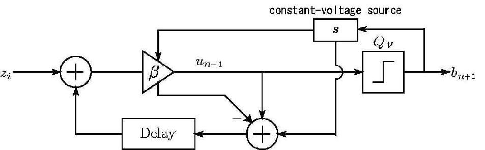
We introduce an A/D converter, called a scale-adjusted β\beta-encoder, that realizes the above expansion, as shown in Fig. 13, where the scale ss of Sβ,ν,sS_{\beta,\nu,s} can be adjusted with the bit-controlled constant-current source of the quantiser s⁡(b)s(b), defined by

s⁡(b)={0,b=0,s,b=1.s(b)=\left\{\begin{array}[]{ll}0,&b=0,\\ s,&b=1.\end{array}\right. (89)

Its robustness to the fluctuation of the quantiser threshold ν\nu is restricted by its tolerance σβ,s\sigma_{\beta,s}:

σβ,s=s−s⁡(β−1)=s⁡(2−β).\sigma_{\beta,s}=s-s(\beta-1)=s(2-\beta). (90)

Even if the amplification factor β\beta is constant, the tolerance σβ,s\sigma_{\beta,s} can be set arbitrarily by selecting the constant-voltage source ss. We get the following convenient lemma as a rule of thumb for AD/DA-converter designs.

Lemma 33: In a scale adjusted β\beta-encoder, for a given bit budget LL and quantiser tolerance σβ,s\sigma_{\beta,s}, the amplification factor β\beta with its inevitable fluctuation, should be set to

β=2​LL+1.\beta=\dfrac{2L}{L+1}. (91)

in order to minimize the quantisation error.

proof: Eq.(86) gives |IL,Sβ,ν,sL​(x)|=s​β−L=σβ,s​β−L(2−β)|I_{L,S^{L}_{\beta,\nu,s}}(x)|=s\beta^{-L}=\dfrac{\sigma_{\beta,s}\beta^{-L}}{(2-\beta)}. Differentiating |IL,Sβ,ν,sL​(x)||I_{L,S^{L}_{\beta,\nu,s}}(x)| with respect to β\beta, we obtain

d​|IL,Sβ,ν,sL​(x)|d​β=σβ,s​β−L−1(2−β)2​{β−L⁡(2−β)}.\dfrac{d|I_{L,S^{L}_{\beta,\nu,s}}(x)|}{d\beta}=\dfrac{\sigma_{\beta,s}\beta^{-L-1}}{(2-\beta)^{2}}\{\beta-L(2-\beta)\}. (92)

This completes the proof. □\Box

This lemma shows that the amplification factor β\beta minimizing the quantisation error is not equal to 22 but the relation β=2\beta=2 as in PCM holds only as L→∞L\rightarrow\infty. However, we must take a little care at this point. Assume that for a given initial value of an A/D converter x∈[0,1)x\in[0,1), the scale s=σβ,s​(L+1)/2>1s=\sigma_{\beta,s}(L+1)/2>1. In this case, we should adjust the amplification factor and the constant-voltage source which satisfy β=2​L/(L+1)\beta=2L/(L+1) and s=σβ,s​(L+1)/2s=\sigma_{\beta,s}(L+1)/2, respectively; otherwise we should adjust these parameters such as s=1s=1 and β=2−sσβ,s=2−σβ,s−1\beta=2-\dfrac{s}{\sigma_{\beta,s}}=2-\sigma_{\beta,s}^{-1}.

Refer to caption
Fig. 12: The scale-adjusted β\beta-map Sβ,ν,s​(x)S_{\beta,\nu,s}(x) with its invariant subinterval [ν−s(β−1),ν)[\nu-s(\beta-1),\nu).
Refer to caption
Fig. 13: The scale-adjusted β\beta-encoder, where s=s⁡(b)s=s(b) is defined by Eq.(89).

VII Negative β\beta-encoder

Refer to caption
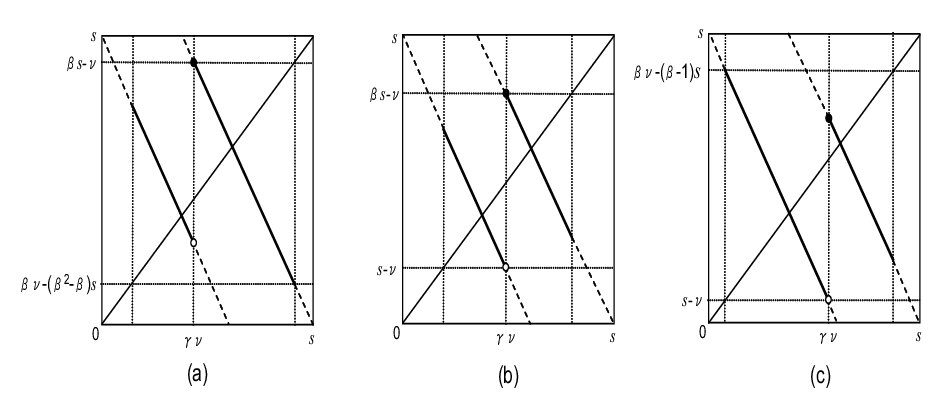
Fig. 14: The map of the negative β\beta-expansion:Rβ,ν,s​(x)R_{\beta,\nu,s}(x). Its invariant subinterval is a function of ν\nu (see Figs. 16(a),(b),(c) and 17(b)).
Refer to caption
Fig. 15: The negative β\beta-encoder.

This section introduces a radix expansion of a real number in a negative real base, called a negative β\beta-expansion, and discusses differences between the quantisation errors of negative β\beta-expansions and those of (scale-adjusted) β\beta-expansions as well as their MSE. Such a negative radix expansion is unusual, and somewhat intricate. First, consider a (scale-adjusted) negative β\beta-expansion as a map Rβ,ν,s​(x):[0,s)→[0,s),s>0R_{\beta,\nu,s}(x):[0,s)\rightarrow[0,s),\,s>0, defined by

Rβ,ν,s​(x)={s−β​x,x∈[0,γ​ν),β​s−β​x,x∈[γ​ν,s),​ν∈[s⁡(β−1),s]\hskip-11.38109ptR_{\beta,\nu,s}(x)=\left\{\begin{array}[]{ll}s-\beta x,&\hskip-5.69054ptx\in[0,\gamma\nu),\\ \beta s-\beta x,&\hskip-5.69054ptx\in[\gamma\nu,s),\\ \end{array}\right.\nu\in[s(\beta-1),s] (93)

as shown in Fig. 14. Such a negative β\beta-expansion defines a new A/D converter as shown in Fig.15, called a negative β\beta-encoder which facilitates the implementation of stable analog circuits 55 5 Personal communication with Prof. Yoshihiko Horio. and improves the quantisation MSE both in the greedy case ν=s⁡(β−1)\nu=s(\beta-1) and in the lazy case ν=s\nu=s as follows. Let bi,Rβ,ν1i,si​(x)b_{i,R^{i}_{\beta,\nu_{1}^{i},s}}(x) be the associated bit sequence for the threshold sequence ν1L\nu_{1}^{L}, defined as

bi,Rβ,ν1i,si​(x)={0,Rβ,ν1i−1,si−1​(x)∈[0,γ​νi),1,Rβ,ν1i−1,si−1​(x)∈[γ​νi,s),b_{i,R^{i}_{\beta,\nu_{1}^{i},s}}(x)=\left\{\begin{array}[]{ll}0,&R_{\beta,\nu_{1}^{i-1},s}^{i-1}(x)\in[0,\gamma\nu_{i}),\\ 1,&R_{\beta,\nu_{1}^{i-1},s}^{i-1}(x)\in[\gamma\nu_{i},s),\end{array}\right. (94)

where Rβ,ν1i,si​(x)R^{i}_{\beta,\nu_{1}^{i},s}(x) is defined recursively as

Rβ,ν1LL​(x)=Rβ,νL​(Rβ,ν1L−1L−1​(x))\displaystyle R^{L}_{\beta,\nu_{1}^{L}}(x)=R_{\beta,\nu_{L}}(R^{L-1}_{\beta,\nu_{1}^{L-1}}(x))
=Rβ,νL(Rβ,νL−1(Rβ,ν1L−2L−2(⋯(Rβ,ν1(x))).\displaystyle=R_{\beta,\nu_{L}}(R_{\beta,\nu_{L-1}}(R^{L-2}_{\beta,\nu_{1}^{L-2}}(\cdots(R_{\beta,\nu_{1}}(x))). (95)

The scale-adjusted negative β\beta map Rβ,ν,s​(x)R_{\beta,\nu,s}(x) also defines the flaky quantiser Q[s⁡(1−γ),s​γ]f​(⋅)Q^{f}_{[s(1-\gamma),s\gamma]}(\cdot). Then Rβ,ν1L,sL​(x)R_{\beta,\nu_{1}^{L},s}^{L}(x) can be represented recursively as follows:

Rβ,ν,sL​(x)=s​fL,Rβ,ν1L,sL−β​Rβ,ν1L−1,sL−1​(x)\displaystyle\hskip-5.69054ptR_{\beta,\nu,s}^{L}(x)=sf_{L,R^{L}_{\beta,\nu_{1}^{L},s}}-\beta R_{\beta,\nu_{1}^{L-1},s}^{L-1}(x) (96)
=\displaystyle= s​fL,Rβ,ν1L,sL−β​s​fL−1,Rβ,ν1L−1,sL−1\displaystyle\hskip-5.69054ptsf_{L,R^{L}_{\beta,\nu_{1}^{L},s}}-\beta sf_{L-1,R^{L-1}_{\beta,\nu_{1}^{L-1},s}}
+\displaystyle+ ⋯+(−β)L−1​s​f1,Rβ,ν11,s+(−β)L​x\displaystyle\hskip-5.69054pt\cdots+(-\beta)^{L-1}sf_{1,R_{\beta,\nu_{1}^{1},s}}+(-\beta)^{L}x
=\displaystyle= s​∑i=1Lfi,Rβ,ν1i,si​(−β)L−i+(−β)L​x\displaystyle\hskip-5.69054pts\sum^{L}_{i=1}f_{i,R^{i}_{\beta,\nu_{1}^{i},s}}(-\beta)^{L-i}+(-\beta)^{L}x

which yields

x=(−γ)L​Rβ,ν1L,sL​(x)−s​∑i=1Lfi,Rβ,ν1i,si​(−γ)i,x=(-\gamma)^{L}R^{L}_{\beta,\nu_{1}^{L},s}(x)-s\sum^{L}_{i=1}f_{i,R^{i}_{\beta,\nu_{1}^{i},s}}(-\gamma)^{i}, (97)

where

fi,Rβ,ν1i,si=1+bi,Rβ,ν1i,si​(β−1).f_{i,R^{i}_{\beta,\nu_{1}^{i},s}}=1+b_{i,R^{i}_{\beta,\nu_{1}^{i},s}}(\beta-1). (98)

The relation Rβ,ν1L,sL​(x)∈[0,s)R^{L}_{\beta,\nu_{1}^{L},s}(x)\in[0,s) defines its subinterval,

I2​L+1,Rβ,ν12​L+1,s2​L+1​(x)\displaystyle I_{2L+1,R^{2L+1}_{\beta,\nu_{1}^{2L+1},s}}(x) (100)
=\displaystyle= s[−γ2​L+1−∑i=12​L+1fi,Rβ,ν1i,si(−γ)i,−∑i=12​L+1fi,Rβ,ν1i,si(−γ)i)\displaystyle\hskip-8.53581pts[-\gamma^{2L+1}-\sum^{2L+1}_{i=1}f_{i,R^{i}_{\beta,\nu_{1}^{i},s}}(-\gamma)^{i},-\sum^{2L+1}_{i=1}f_{i,R^{i}_{\beta,\nu_{1}^{i},s}}(-\gamma)^{i})
I2​L,Rβ,ν12​L,s2​L​(x)\displaystyle I_{2L,R^{2L}_{\beta,\nu_{1}^{2L},s}}(x)
=\displaystyle= s[−∑i=12​Lfi,Rβ,ν1i,si(−γ)i,γ2​L−∑i=12​Lfi,Rβ,ν1i,si(−γ)i)\displaystyle\hskip-8.53581pts[-\sum^{2L}_{i=1}f_{i,R^{i}_{\beta,\nu_{1}^{i},s}}(-\gamma)^{i},\gamma^{2L}-\sum^{2L}_{i=1}f_{i,R^{i}_{\beta,\nu_{1}^{i},s}}(-\gamma)^{i})

which enables us to obtain the following decoded value x^L,Rβ,ν1L,s\widehat{x}_{L,R_{\beta,\nu_{1}^{L},s}}:

x^L,Rβ,ν1L,sL=s⁡{(−γ)L/2−∑i=1Lfi,Rβ,ν1i,si​(−γ)i}.\widehat{x}_{L,R^{L}_{\beta,\nu_{1}^{L},s}}=s\{(-\gamma)^{L}/2-\sum^{L}_{i=1}f_{i,R^{i}_{\beta,\nu_{1}^{i},s}}(-\gamma)^{i}\}. (101)

Then, its quantisation error ϵL,Rβ,ν1L,sL​(x)\epsilon_{L,R^{L}_{\beta,\nu_{1}^{L},s}}(x) is bounded as

ϵL,Rβ,ν1L,sL​(x)=|x−x^L,Rβ,ν1L,sL|≤s​γL2,\epsilon_{L,R^{L}_{\beta,\nu_{1}^{L},s}}(x)=|x-\widehat{x}_{L,R^{L}_{\beta,\nu_{1}^{L},s}}|\leq\dfrac{s\gamma^{L}}{2}, (102)

which is the same as in the scale-adjusted β\beta-expansion.

Such a successive approximation of xx by the cautious expansion using ν1L\nu_{1}^{L} is described by the contraction process of the interval by the negative β\beta-expansion as follows. Let Ii,Rβ,ν1i,si​(x)=[liR​(ν1i),riR​(ν1i)),i≥1I_{i,R^{i}_{\beta,\nu_{1}^{i},s}}(x)=[l^{R}_{i}(\nu_{1}^{i}),r^{R}_{i}(\nu_{1}^{i})),\,i\geq 1 be the i​thi\mbox{th} interval for the negative β\beta-expansion map Rβ,νi,s​(x)R_{\beta,\nu_{i},s}(x) with the threshold sequence ν1i,(s⁡(β−1)≤νj≤s)\nu_{1}^{i},(s(\beta-1)\leq\nu_{j}\leq s), recursively defined by

l2​ℓ+1R​(ν12​ℓ+1)=l2​ℓR​(ν12​ℓ)−s​γ2​ℓ+1​(1−f2​ℓ+1,Rβ,ν12​ℓ+1,s2​ℓ+1),r2​ℓ+1R​(ν12​ℓ+1)=r2​ℓR​(ν12​ℓ)−s​γ2​ℓ​(1−f2​ℓ+1,Rβ,ν12​ℓ+1,s2​ℓ+1​γ),l2​ℓR​(ν12​ℓ)=l2​ℓ−1R​(ν12​ℓ−1)+s​γ2​ℓ−1​(1−f2​ℓ,Rβ,ν12​ℓ,s2​ℓ​γ),r2​ℓR​(ν12​ℓ)=r2​ℓ−1R​(ν12​ℓ−1)+s​γ2​ℓ​(1−f2​ℓ,Rβ,ν12​ℓ,s2​ℓ).\begin{array}[]{lcr}l^{R}_{2\ell+1}(\nu_{1}^{2\ell+1})&=&l^{R}_{2\ell}(\nu_{1}^{2\ell})-s\gamma^{2\ell+1}(1-f_{2\ell+1,R^{2\ell+1}_{\beta,\nu_{1}^{2\ell+1},s}}),\\ r^{R}_{2\ell+1}(\nu_{1}^{2\ell+1})&=&r^{R}_{2\ell}(\nu_{1}^{2\ell})-s\gamma^{2\ell}(1-f_{2\ell+1,R^{2\ell+1}_{\beta,\nu_{1}^{2\ell+1},s}}\gamma),\\ l^{R}_{2\ell}(\nu_{1}^{2\ell})&=&l^{R}_{2\ell-1}(\nu_{1}^{2\ell-1})+s\gamma^{2\ell-1}(1-f_{2\ell,R^{2\ell}_{\beta,\nu_{1}^{2\ell},s}}\gamma),\\ r^{R}_{2\ell}(\nu_{1}^{2\ell})&=&r^{R}_{2\ell-1}(\nu_{1}^{2\ell-1})+s\gamma^{2\ell}(1-f_{2\ell,R^{2\ell}_{\beta,\nu_{1}^{2\ell},s}}).\\ \end{array} (103)

Thus, we have the following lemma.

Lemma 44 : If x∈Ii,Rβ,ν1i,si​(x)x\in I_{i,R^{i}_{\beta,\nu_{1}^{i},s}}(x), then x∈Ii+1,Rβ,ν1i+1,si+1​(x),i∈ℤx\in I_{i+1,R^{i+1}_{\beta,\nu_{1}^{i+1},s}}(x),\,\,i\in\mathbb{Z}.

proof: It is obvious that x∈I0,Rβ,ν,s​(x)=[0,s)x\in I_{0,R_{\beta,\nu,s}}(x)=[0,s) because x∈[0,1)⊂I0,Rβ,ν​(x)x\in[0,1)\subset I_{0,R_{\beta,\nu}}(x). Suppose that x∈I2​ℓ,Rβ,ν12​ℓ,s2​ℓ​(x)x\in I_{2\ell,R^{2\ell}_{\beta,\nu_{1}^{2\ell},s}}(x). Then,

x−l2​ℓ+1R​(ν12​ℓ+1)\displaystyle\hskip-5.69054ptx-l^{R}_{2\ell+1}(\nu_{1}^{2\ell+1})
=\displaystyle= γ2​ℓ​Rβ,ν12​ℓ,s2​ℓ​(x)−s​∑i=12​ℓfi,Rβ,ν1i,si​(−γ)i\displaystyle\hskip-5.69054pt\gamma^{2\ell}R^{2\ell}_{\beta,\nu_{1}^{2\ell},s}(x)-s\displaystyle{\sum_{i=1}^{2\ell}f_{i,R^{i}_{\beta,\nu_{1}^{i},s}}(-\gamma)^{i}}
−\displaystyle- l2​ℓR​(ν12​ℓ)+s​γ2​ℓ+1​(1−f2​ℓ+1,Rβ,ν12​ℓ+1,s2​ℓ+1)\displaystyle\hskip-5.69054ptl^{R}_{2\ell}(\nu_{1}^{2\ell})+s\gamma^{2\ell+1}(1-f_{2\ell+1,R^{2\ell+1}_{\beta,\nu_{1}^{2\ell+1},s}})
=\displaystyle= γ2​ℓ​{Rβ,ν12​ℓ,s2​ℓ​(x)+s​γ​(1−f2​ℓ+1,Rβ,ν12​ℓ+1,s2​ℓ+1)},\displaystyle\hskip-5.69054pt\gamma^{2\ell}\{R^{2\ell}_{\beta,\nu_{1}^{2\ell},s}(x)+s\gamma(1-f_{2\ell+1,R^{2\ell+1}_{\beta,\nu_{1}^{2\ell+1},s}})\},

which suggests that if Rβ,ν12​ℓ,s2​ℓ​(x)<γ​ν2​ℓ+1,i.e.,R^{2\ell}_{\beta,\nu_{1}^{2\ell},s}(x)<\gamma\nu_{2\ell+1},\mbox{{\it i.e.,}} f2​ℓ+1,Rβ,ν12​ℓ+1,s2​ℓ+1=1f_{2\ell+1,R^{2\ell+1}_{\beta,\nu_{1}^{2\ell+1},s}}=1, then x−l2​ℓ+1R​(ν12​ℓ+1)=γ2​ℓ​Rβ,ν12​ℓ,s2​ℓ​(x)≥0x-l^{R}_{2\ell+1}(\nu_{1}^{2\ell+1})=\gamma^{2\ell}R^{2\ell}_{\beta,\nu_{1}^{2\ell},s}(x)\geq 0. Otherwise i.e.,​f2​ℓ+1,Rβ,ν12​ℓ+1,s2​ℓ+1=β\mbox{{\it i.e.,}}\,f_{2\ell+1,R^{2\ell+1}_{\beta,\nu_{1}^{2\ell+1},s}}=\beta, x−l2​ℓ+1R​(ν12​ℓ+1)≥γ2​ℓ+1​{ν2​ℓ+1−s⁡(β−1)}≥0x-l^{R}_{2\ell+1}(\nu_{1}^{2\ell+1})\geq\gamma^{2\ell+1}\{\nu_{2\ell+1}-s(\beta-1)\}\geq 0 because ν2​ℓ+1≥s⁡(β−1)\nu_{2\ell+1}\geq s(\beta-1). On the other hand,

r2​ℓ+1R​(ν12​ℓ+1)−x\displaystyle\hskip-8.53581ptr^{R}_{2\ell+1}(\nu_{1}^{2\ell+1})-x
=\displaystyle= r2​ℓR​(ν12​ℓ)−s​γ2​ℓ​(1−f2​ℓ+1,Rβ,ν12​ℓ+1,s2​ℓ+1​γ)\displaystyle\hskip-8.53581ptr^{R}_{2\ell}(\nu_{1}^{2\ell})-s\gamma^{2\ell}(1-f_{2\ell+1,R^{2\ell+1}_{\beta,\nu_{1}^{2\ell+1},s}}\gamma)
−\displaystyle- {γ2​ℓ​Rβ,ν12​ℓ,s2​ℓ​(x)−s​∑i=12​ℓfi,Rβ,ν1i,si​(−γ)i}\displaystyle\hskip-8.53581pt\{\gamma^{2\ell}R^{2\ell}_{\beta,\nu_{1}^{2\ell},s}(x)-s\displaystyle{\sum_{i=1}^{2\ell}f_{i,R^{i}_{\beta,\nu_{1}^{i},s}}(-\gamma)^{i}}\}
=\displaystyle= s​γ2​ℓ+1​f2​ℓ+1,Rβ,ν12​ℓ+1,s2​ℓ+1−γ2​ℓ​Rβ,ν12​ℓ,s2​ℓ​(x)\displaystyle\hskip-8.53581pts\gamma^{2\ell+1}f_{2\ell+1,R^{2\ell+1}_{\beta,\nu_{1}^{2\ell+1},s}}-\gamma^{2\ell}R^{2\ell}_{\beta,\nu_{1}^{2\ell},s}(x)
=\displaystyle= γ2​ℓ​{s​γ​f2​ℓ+1,Rβ,ν12​ℓ+1,s2​ℓ+1−Rβ,ν12​ℓ,s2​ℓ​(x)},\displaystyle\hskip-5.69054pt\gamma^{2\ell}\{s\gamma f_{2\ell+1,R^{2\ell+1}_{\beta,\nu_{1}^{2\ell+1},s}}-R^{2\ell}_{\beta,\nu_{1}^{2\ell},s}(x)\},

which suggests that if Rβ,ν12​ℓ,s2​ℓ​(x)<γ​ν2​ℓ+1R^{2\ell}_{\beta,\nu_{1}^{2\ell},s}(x)<\gamma\nu_{2\ell+1}, i.e., f2​ℓ+1,Rβ,ν12​ℓ+1,s2​ℓ+1=1f_{2\ell+1,R^{2\ell+1}_{\beta,\nu_{1}^{2\ell+1},s}}=1, then r2​ℓ+1R​(ν12​ℓ+1)−x≥γ2​ℓ+1​(s−ν2​ℓ+1)≥0r^{R}_{2\ell+1}(\nu_{1}^{2\ell+1})-x\geq\gamma^{2\ell+1}(s-\nu_{2\ell+1})\geq 0 because ν2​ℓ+1<s\nu_{2\ell+1}<s. Otherwise  i.e.,​f2​ℓ+1,Rβ,ν12​ℓ+1,s=β\mbox{{\it i.e.,}}\,f_{2\ell+1,R_{\beta,\nu_{1}^{2\ell+1},s}}=\beta, r2​ℓ​1R​(ν12​ℓ+1)−x≥γ2​ℓ​{s−Rβ,ν12​ℓ,s2​ℓ​(x)}≥0r^{R}_{2\ell 1}(\nu_{1}^{2\ell+1})-x\geq\gamma^{2\ell}\{s-R^{2\ell}_{\beta,\nu_{1}^{2\ell},s}(x)\}\geq 0 because OPENRβ,ν12​ℓ,s2​ℓ​(x))≤sR^{2\ell}_{\beta,\nu_{1}^{2\ell},s}(x))\leq s. This implies that x∈I2​ℓ+1,Rβ,ν12​ℓ+1,s2​ℓ+1​(x).x\in I_{2\ell+1,R^{2\ell+1}_{\beta,\nu_{1}^{2\ell+1},s}}(x).
Similarly, suppose that x∈I2​ℓ−1,Rβ,ν12​ℓ−12​ℓ−1​(x)x\in I_{2\ell-1,R^{2\ell-1}_{\beta,\nu_{1}^{2\ell-1}}}(x). Then,

x−l2​ℓR​(ν12​ℓ)\displaystyle\hskip-5.69054ptx-l^{R}_{2\ell}(\nu_{1}^{2\ell})
=\displaystyle= −γ2​ℓ−1​Rβ,ν12​ℓ−1,s2​ℓ−1​(x)−s​∑i=12​ℓ−1fi,Rβ,ν1i,si​(−γ)i\displaystyle\hskip-5.69054pt-\gamma^{2\ell-1}R^{2\ell-1}_{\beta,\nu_{1}^{2\ell-1},s}(x)-s\displaystyle{\sum_{i=1}^{2\ell-1}f_{i,R^{i}_{\beta,\nu_{1}^{i},s}}(-\gamma)^{i}}
+\displaystyle+ s​∑i=12​ℓfi,Rβ,ν1i,si​(−γ)i\displaystyle\hskip-5.69054pts\displaystyle{\sum_{i=1}^{2\ell}f_{i,R^{i}_{\beta,\nu_{1}^{i},s}}(-\gamma)^{i}}
=\displaystyle= γ2​ℓ−1​{s​γ​f2​ℓ,Rβ,ν12​ℓ,s2​ℓ−Rβ,ν12​ℓ−1,s2​ℓ−1​(x)},\displaystyle\hskip-5.69054pt\gamma^{2\ell-1}\{s\gamma f_{2\ell,R_{\beta,\nu_{1}^{2\ell},s}^{2\ell}}-R^{2\ell-1}_{\beta,\nu_{1}^{2\ell-1},s}(x)\},

which suggests that if Rβ,ν12​ℓ−12​ℓ−1​(x)<γ​ν2​ℓ,i.e.,​f2​ℓ,Rβ,ν12​ℓ,s2​ℓ=1R^{2\ell-1}_{\beta,\nu_{1}^{2\ell-1}}(x)<\gamma\nu_{2\ell},\,\mbox{{\it i.e.,}}\,f_{2\ell,R_{\beta,\nu_{1}^{2\ell},s}^{2\ell}}=1, then x−l2​ℓR​(ν12​ℓ)=γ2​ℓ​(s−ν2​ℓ)≥0x-l^{R}_{2\ell}(\nu_{1}^{2\ell})=\gamma^{2\ell}(s-\nu_{2\ell})\geq 0 because ν2​ℓ≤s\nu_{2\ell}\leq s. Otherwise  i.e.,​f2​ℓ,Rβ,ν12​ℓ,s2​ℓ=β\mbox{{\it i.e.,}}f_{2\ell,R_{\beta,\nu_{1}^{2\ell},s}^{2\ell}}=\beta, x−l2​ℓR​(ν12​ℓ)=γ2​ℓ−1​{s−Rβ,ν12​ℓ−1,s2​ℓ−1​(x)}≥0x-l^{R}_{2\ell}(\nu_{1}^{2\ell})=\gamma^{2\ell-1}\{s-R^{2\ell-1}_{\beta,\nu_{1}^{2\ell-1},s}(x)\}\geq 0 because Rβ,ν12​ℓ−1,s2​ℓ−1​(x)≤sR^{2\ell-1}_{\beta,\nu_{1}^{2\ell-1},s}(x)\leq s. On the other hand,

r2​ℓR​(ν12​ℓ)−x\displaystyle\hskip-5.69054ptr^{R}_{2\ell}(\nu_{1}^{2\ell})-x
=\displaystyle= r2​ℓ−1R​(ν12​ℓ−1)+s​γ2​ℓ​(1−f2​ℓ,Rβ,ν12​ℓ,s2​ℓ)\displaystyle\hskip-5.69054ptr^{R}_{2\ell-1}(\nu_{1}^{2\ell-1})+s\gamma^{2\ell}(1-f_{2\ell,R^{2\ell}_{\beta,\nu_{1}^{2\ell},s}})
+\displaystyle+ γ2​ℓ−1​Rβ,ν12​ℓ−1,s2​ℓ−1​(x)+s​∑i=12​ℓ−1fi,Rβ,ν1i,si​(−γ)i\displaystyle\hskip-5.69054pt\gamma^{2\ell-1}R^{2\ell-1}_{\beta,\nu_{1}^{2\ell-1},s}(x)+s\displaystyle{\sum_{i=1}^{2\ell-1}f_{i,R^{i}_{\beta,\nu_{1}^{i},s}}(-\gamma)^{i}}
=\displaystyle= γ2​ℓ−1​{s​γ​(1−f2​ℓ,Rβ,ν12​ℓ,s2​ℓ)+Rβ,ν12​ℓ−1,s2​ℓ−1​(x)},\displaystyle\hskip-5.69054pt\gamma^{2\ell-1}\{s\gamma(1-f_{2\ell,R^{2\ell}_{\beta,\nu_{1}^{2\ell},s}})+R^{2\ell-1}_{\beta,\nu_{1}^{2\ell-1},s}(x)\},

which implies that if Rβ,ν12​ℓ−1,s2​ℓ−1​(x)<γ​ν2​ℓ,i.e.,​f2​ℓ,Rβ,ν12​ℓ,s2​ℓ=1R^{2\ell-1}_{\beta,\nu_{1}^{2\ell-1},s}(x)<\gamma\nu_{2\ell},\mbox{{\it i.e.,}}f_{2\ell,R^{2\ell}_{\beta,\nu_{1}^{2\ell},s}}=1, then r2​ℓR​(ν12​ℓ,s)−x=γ2​ℓ−1​Rβ,ν12​ℓ−1,s2​ℓ−1​(x)≥0r_{2\ell}^{R}(\nu_{1}^{2\ell},s)-x=\gamma^{2\ell-1}R^{2\ell-1}_{\beta,\nu_{1}^{2\ell-1},s}(x)\geq 0. Otherwise,  i.e.,​f2​ℓ,Rβ,ν12​ℓ,s2​ℓ=β,r2​ℓR​(ν12​ℓ)−x≥γ2​ℓ​{−s⁡(β−1)+ν2​ℓ}≥0\mbox{{\it i.e.,}}f_{2\ell,R^{2\ell}_{\beta,\nu_{1}^{2\ell},s}}=\beta,r^{R}_{2\ell}(\nu_{1}^{2\ell})-x\geq\gamma^{2\ell}\{-s(\beta-1)+\nu_{2\ell}\}\geq 0 because s⁡(β−1)≤ν2​ℓs(\beta-1)\leq\nu_{2\ell}. This implies that x∈I2​ℓ,Rβ,ν12​ℓ2​ℓ,s​(x).x\in I_{2\ell,R^{2\ell}_{\beta,\nu_{1}^{2\ell}},s}(x). This completes the proof. □\Box

Similarly, using the idea of Daubechies et al. and the negative β\beta-expansion sequences bi,Rβ,ν1i,sib_{i,R^{i}_{\beta,\nu_{1}^{i},s}} for xx and ci,Rβ,ν1i,sic_{i,R^{i}_{\beta,\nu_{1}^{i},s}} for y=1−xy=1-x (i=1,2,⋯,L)(i=1,2,\cdots,L), we can get the characteristic equation of β\beta in a negative β\beta-encoder as follows:

PL,Rβ,ν1L,sL​(γ)\displaystyle\hskip-8.53581ptP_{L,R^{L}_{\beta,\nu_{1}^{L},s}}(\gamma) (104)
=\displaystyle= s⁡{(−γ)L−∑i=1L(2+{bi,Rβ,ν1i,si+ci,Rβ,ν1i,si}​(β−1))​(−γ)i}−1\displaystyle\hskip-8.53581pts\{(-\gamma)^{L}-\hskip-2.84526pt\sum^{L}_{i=1}(2+\{b_{i,R^{i}_{\beta,\nu_{1}^{i},s}}+c_{i,R^{i}_{\beta,\nu_{1}^{i},s}}\}(\beta-1))(-\gamma)^{i}\}-1
=\displaystyle= s{[dL,Rβ,ν1L,sL−1](−γ)L\displaystyle\hskip-8.53581pts\{[d_{L,R^{L}_{\beta,\nu_{1}^{L},s}}-1](-\gamma)^{L}
−\displaystyle- ∑i=1L−1[2−di,Rβ,ν1i,si+di+1,Rβ,ν1i+1,si+1](−γ)i}−1,\displaystyle\hskip-8.53581pt\hskip-2.84526pt\sum^{L-1}_{i=1}[2-d_{i,R^{i}_{\beta,\nu_{1}^{i},s}}+d_{i+1,R^{i+1}_{\beta,\nu_{1}^{i+1},s}}](-\gamma)^{i}\}-1,

where di,Rβ,ν1i,si=bi,Rβ,ν1i,si+ci,Rβ,ν1i,sid_{i,R^{i}_{\beta,\nu_{1}^{i},s}}=b_{i,R^{i}_{\beta,\nu_{1}^{i},s}}+c_{i,R^{i}_{\beta,\nu_{1}^{i},s}}. However, it is hard to guarantee the uniqueness of the root of Eq.(104).

The invariant subinterval of the map Rβ,ν,s​(x)R_{\beta,\nu,s}(x) consists of 2 line segments as shown in Fig.14. The line segment in the graph of Rβ,ν,s​(x)R_{\beta,\nu,s}(x) with the full range is called a full line segment. 66 6 In the β\beta-expansion, the greedy-expansion map (or the lazy-expansion map), restricted to its invariant subinterval has a left (or right) full line segment as shown in Fig.4 (a) (or (b)) but the cautious-expansion map, restricted to its invariant subinterval has no full line segment as shown in Fig.3 (a). There are three possible cases as follows:

  1. 1.

    The right segment is the full line segment (as shown in Fig. 16(a)) whose invariant subinterval is given by

    [βν−(β2−β)s,βs−ν)[\beta\nu-(\beta^{2}-\beta)s,\beta s-\nu) (105)

    when (β−1)​s≤ν<β2−β+1β+1​s(\beta-1)s\leq\nu<\dfrac{\beta^{2}-\beta+1}{\beta+1}s since

    β​s−ν−{β​ν−(β2−β)​s}>β​s−ν−{s−ν}\displaystyle\hskip-39.83385pt\beta s-\nu-\{\beta\nu-(\beta^{2}-\beta)s\}>\beta s-\nu-\{s-\nu\}
    ⇔\displaystyle\Leftrightarrow (β2−β+1)​s−(β+1)​ν>0\displaystyle(\beta^{2}-\beta+1)s-(\beta+1)\nu>0
    ⇔\displaystyle\Leftrightarrow ν<β2−β+1β+1​s.\displaystyle\nu<\dfrac{\beta^{2}-\beta+1}{\beta+1}s.
  2. 2.

    No full line segment (as shown in Fig. 16(b)) whose invariant subinterval is given by

    [s−ν,βs−ν),[s-\nu,\beta s-\nu), (106)

    when β2−β+1β+1​s≤ν<2​β−1β+1​s\dfrac{\beta^{2}-\beta+1}{\beta+1}s\leq\nu<\dfrac{2\beta-1}{\beta+1}s since

    β​s−ν−(s−ν)=(β−1)​s>β​ν−(β−1)​s−(s−ν)\displaystyle\hskip-28.45274pt\beta s-\nu-(s-\nu)=(\beta-1)s>\beta\nu-(\beta-1)s-(s-\nu)
    ⇔\displaystyle\Leftrightarrow (2​β−1)​s>(β+1)​ν.\displaystyle(2\beta-1)s>(\beta+1)\nu.
    ⇔\displaystyle\Leftrightarrow ν<2​β−1β+1​s.\displaystyle\nu<\dfrac{2\beta-1}{\beta+1}s.
  3. 3.

    The left segment is the full line segment (as shown in Fig. 16(c)) whose invariant subinterval is given by

    [s−ν,βν−s(β−1)),[s-\nu,\beta\nu-s(\beta-1)), (107)

    when 2​β−1β+1​s≤ν≤s\dfrac{2\beta-1}{\beta+1}s\leq\nu\leq s since

    β​ν−(β−1)​s−{s−ν}≥β​s−ν−(s−ν)\displaystyle\hskip-28.45274pt\beta\nu-(\beta-1)s-\{s-\nu\}\geq\beta s-\nu-(s-\nu)
    ⇔\displaystyle\Leftrightarrow (β+1)​ν−(2​β−1)​s≥0\displaystyle(\beta+1)\nu-(2\beta-1)s\geq 0
    ⇔\displaystyle\Leftrightarrow 2​β−1β+1​s≤ν.\displaystyle\dfrac{2\beta-1}{\beta+1}s\leq\nu.
Refer to caption
Fig. 16: Negative β\beta-expansion map Rβ,ν,s​(x)R_{\beta,\nu,s}(x) with its invariant subinterval when (a) (β−1)​s≤ν<β2−β+1β+1​s(\beta-1)s\leq\nu<\dfrac{\beta^{2}-\beta+1}{\beta+1}s, (b) β2−β+1β+1​s≤ν<2​β−1β+1​s\dfrac{\beta^{2}-\beta+1}{\beta+1}s\leq\nu<\dfrac{2\beta-1}{\beta+1}s, and (c) 2​β−1β+1​s≤ν≤s\dfrac{2\beta-1}{\beta+1}s\leq\nu\leq s.
Refer to caption
Fig. 17: Invariant subinterval, a function of ν\nu, in (a) an ordinary β\beta-expansion (see Fig.4(a),(b)) and (b) a negative β\beta-expansion (see Fig.16(a),(b),(c)) .
Refer to caption
Fig. 18: The MSE​(x^L,Rβ,ν1L,sL​(γ,1))\mbox{MSE}(\widehat{x}_{L,R^{L}_{\beta,\nu_{1}^{L},s}}(\gamma,1)) using the exact β\beta of the negative β\beta-encoder with β=1.5\beta=1.5, L=16L=16, and s=(β−1)−1s=(\beta-1)^{-1} for fluctuating νi, 1≤i≤L\nu_{i},\,1\leq i\leq L  with its fluctuations 0,20,30,40%0,20,30,40\%.
Refer to caption
Fig. 19: The MSE of the estimated β\beta, i.e., β^L,Rβ,ν1LL,s​(γ,1)\widehat{\beta}_{L,R^{L}_{\beta,\nu_{1}^{L}},s}(\gamma,1) of the negative β\beta-encoder with β=1.5\beta=1.5, L=16L=16 and s=(β−1)−1s=(\beta-1)^{-1} for fluctuating νi, 1≤i≤L\nu_{i},\,1\leq i\leq L  with its fluctuations 0,20,30,40%0,20,30,40\%.
Refer to caption
Fig. 20: The MSE​(x^L,Rβ,ν1L,sL​(γ^,1))\mbox{MSE}(\widehat{x}_{L,R^{L}_{\beta,\nu_{1}^{L},s}}(\widehat{\gamma},1)) using the estimated β^\widehat{\beta} of the negative β\beta-encoder with β=1.5\beta=1.5, L=16L=16, and s=(β−1)−1s=(\beta-1)^{-1} for fluctuating νi, 1≤i≤L\nu_{i},\,1\leq i\leq L  with its fluctuations 0,20,30,40%0,20,30,40\%.
Refer to caption
Fig. 21: The MSE​(x^L,Cβ,ν∗L​(γ,1))\mbox{MSE}(\widehat{x}_{L,C^{L}_{\beta,\nu^{*}}}(\gamma,1)) (or MSE​(x^L,Rβ,ν∗,sL​(γ,1))\mbox{MSE}(\widehat{x}_{L,R^{L}_{\beta,\nu^{*},s}}(\gamma,1)) using the exact β\beta of the β\beta-encoder (or the negative β\beta-encoder) with β=1.5\beta=1.5, L=16L=16, and  s=(β−1)−1s=(\beta-1)^{-1} for fixed ν∗∈[1,(β−1)−1]\nu^{*}\in[1,(\beta-1)^{-1}].
Refer to caption
Fig. 22: The MSE​(x^L,Cβ,ν∗L​(γ^,1))\mbox{MSE}(\widehat{x}_{L,C^{L}_{\beta,\nu^{*}}}(\widehat{\gamma},1)) (or MSE​(x^L,Rβ,ν∗,sL​(γ^,1))\mbox{MSE}(\widehat{x}_{L,R^{L}_{\beta,\nu^{*},s}}(\widehat{\gamma},1))  using the estimated β^\widehat{\beta} of the β\beta-encoder (or the negative β\beta-encoder) with β=1.5\beta=1.5, L=16L=16, and s=(β−1)−1s=(\beta-1)^{-1} for fixed ν∗∈[1,(β−1)−1]\nu^{*}\in[1,(\beta-1)^{-1}].
Refer to caption
Fig. 23: The MSE of the estimated β\beta, i.e., β^L,Cβ,ν∗L​(γ,1)\widehat{\beta}_{L,C^{L}_{\beta,\nu^{*}}}(\gamma,1) ( or β^L,Rβ,ν∗L​(γ,1)\widehat{\beta}_{L,R^{L}_{\beta,\nu^{*}}}(\gamma,1)) of the β\beta-encoder (or the negative β\beta-encoder) with a fixed ν∗∈[1,(β−1)−1]\nu^{*}\in[1,(\beta-1)^{-1}] for β=1.5\beta=1.5, L=16L=16, and s=(β−1)−1s=(\beta-1)^{-1}.

Since the quantisation error in the β\beta-expansion is bounded as

ϵL,Sβ,ν1L,sL​(x)=|x−x^L,Sβ,ν1L,sL​(x)|=γL​|s2−Sβ,ν1L,sL​(x)|,\epsilon_{L,S^{L}_{\beta,\nu_{1}^{L},s}}(x)=|x-\widehat{x}_{L,S^{L}_{\beta,\nu_{1}^{L},s}}(x)|=\gamma^{L}|\dfrac{s}{2}-S^{L}_{\beta,\nu_{1}^{L},s}(x)|, (108)

the MSE of the quantisation decreases if Sβ,ν,s​(x)S_{\beta,\nu,s}(x) frequently takes on values in the middle portion of the interval [0,s)[0,s). It is natural to assert that the quantisation threshold ν\nu (with the inevitable errors) should be designed to be nearly equal to

ν=β​s/2\nu=\beta s/2 (109)

so as to reduce the quantisation MSE (see Figs.  5, 7, 8, 9, 10, 11).
The invariant subinterval in the β\beta-expansion given as [ν−s(β−1),ν)[\nu-s(\beta-1),\nu) as a function of ν\nu is illustrated in Figure 17(a), where the β\beta-expansion is here called the ordinary β\beta-expansion in order to discriminate between the β\beta-expansion and the negative β\beta-expansion. Hence the MSE becomes lower when ν=β​s2\nu=\dfrac{\beta s}{2} since the invariant subinterval is given by [(1−β2)​s,β​s2)[(1-\dfrac{\beta}{2})s,\dfrac{\beta s}{2}). Meanwhile, the MSE in the greedy expansion (ν=s⁡(β−1)\nu=s(\beta-1)) (or the lazy expansion (ν=s\nu=s)) increases because the invariant subinterval is given as [0,(β−1)​s)[0,(\beta-1)s) (or [s⁡(2−β),s)[s(2-\beta),s)), which is skewed towards the left (or the right) portion of the initial interval [0,s)[0,s) as shown in Fig.17(a).

On the other hand, the invariant subinterval in a negative β\beta-expansion as a function of ν\nu is illustrated in Figure 17(b). In particular, both of the greedy expansion and the lazy expansion have as their invariant subintervals, given as [0,s)[0,s), which is the same as the initial subinterval. Therefore, the quantisation MSE automatically becomes lower compared to that of a β\beta-expansion, while the invariant subinterval in a negative β\beta-expansion with ν=β​s/2\nu=\beta s/2 is given by [s⁡(1−β/2),β​s/2][s(1-\beta/2),\beta s/2], which is the same as in a β\beta-expansion with ν=β​s2\nu=\dfrac{\beta s}{2}, so the MSE is comparable. Figures 18 and 19 show the MSE​(x^L,Rβ,ν1L,sL​(γ,1))\mbox{MSE}(\widehat{x}_{L,R^{L}_{\beta,\nu_{1}^{L},s}}(\gamma,1)) using the exact β\beta of the negative β\beta-encoder and the MSE​(β^L,Rβ,ν1L,sL​(x^,1))\mbox{MSE}(\widehat{\beta}_{L,R^{L}_{\beta,\nu_{1}^{L},s}}(\widehat{x},1)), respectively, with β=1.5\beta=1.5, L=16L=16, s=(β−1)−1s=(\beta-1)^{-1} for fluctuating νi, 1≤i≤L\nu_{i},\,1\leq i\leq L  with their several fluctuation bounds. Figure 20 shows the MSE​(x^L,Rβ,ν1L,sL​(γ^,1))\mbox{MSE}(\widehat{x}_{L,R^{L}_{\beta,\nu_{1}^{L},s}}(\widehat{\gamma},1)) using the estimated β^\widehat{\beta} of the negative β\beta-encoder. Comparing Fig.18 with Fig.20 shows that x^L,Rβ,ν1L,sL​(γ^,1)\widehat{x}_{L,R^{L}_{\beta,\nu_{1}^{L},s}}(\widehat{\gamma},1) gives a better approximation to xx than x^L,Rβ,ν1L,sL​(γ,1)\widehat{x}_{L,R^{L}_{\beta,\nu_{1}^{L},s}}(\gamma,1). Figure 21 shows the MSE​(x^L,Cβ,ν1LL​(γ,1))\mbox{MSE}(\widehat{x}_{L,C^{L}_{\beta,\nu_{1}^{L}}}(\gamma,1)) (or MSE​(x^L,Rβ,ν1L,sL​(γ,1))\mbox{MSE}(\widehat{x}_{L,R^{L}_{\beta,\nu_{1}^{L},s}}(\gamma,1))) of quantizations using the exact β\beta of the β\beta-encoder (or the negative β\beta-encoder). Figure 22 shows the MSE​(x^L,Cβ,ν1LL​(γ^,1))\mbox{MSE}(\widehat{x}_{L,C^{L}_{\beta,\nu_{1}^{L}}}(\widehat{\gamma},1)) (or MSE​(x^L,Rβ,ν1L,sL​(γ^,1))\mbox{MSE}(\widehat{x}_{L,R^{L}_{\beta,\nu_{1}^{L},s}}(\widehat{\gamma},1))) using the estimated β^\widehat{\beta} of the β\beta-encoder (or the negative β\beta-encoder) with β=1.5\,\beta=1.5, L=16L=16, s=(β−1)−1s=(\beta-1)^{-1} for fixed ν∗∈[1,(β−1)−1]\nu^{*}\in[1,(\beta-1)^{-1}]. Note that the OPENMSE​(x^L,Cβ,ν1LL​(γ^,1)))\mbox{MSE}(\widehat{x}_{L,C^{L}_{\beta,\nu_{1}^{L}}}(\widehat{\gamma},1))) is smaller than the OPENMSE​(x^L,Rβ,ν1L,sL​(γ,1)))\mbox{MSE}(\widehat{x}_{L,R^{L}_{\beta,\nu_{1}^{L},s}}(\gamma,1))) even though the OPENMSE​(β^L,Rβ,ν1L,sL​(x^,1)))\mbox{MSE}(\widehat{\beta}_{L,R^{L}_{\beta,\nu_{1}^{L},s}}(\widehat{x},1))) is smaller than the OPENMSE​(β^L,Cβ,ν1LL​(x^,1)))\mbox{MSE}(\widehat{\beta}_{L,C^{L}_{\beta,\nu_{1}^{L}}}(\widehat{x},1))) as shown in Fig.23.

VIII Markov chain of binary sequences generated by β\beta-encoder

As discussed above, the localized invariant subinterval makes the quantisation MSE in greedy/lazy-expansions worse than that of the cautious-expansion. Regarding a binary sequence generated by the greedy/lazy and cautious expansions as a Markov chain generating binary sequences, we show another clear distinction between them. Furthermore, we observe that such a Markov chain explains the probabilistic behavior of the flaky quantisers, defined by the multivalued Rényi maps.
First, let us notice that there is a close relationship between information sources and a Markov chain with a transition matrix of a finite dimension [35]. The β\beta-expansion maps, however, are not easy to characterize by transition matrices of size 22 except for the original Rényi map with β=(1+5)/2\beta=(1+\sqrt{5})/2. 77 7 This value is a root of γ=β−1\gamma=\beta-1, which comes from the sufficient condition for the greedy map to be a two-state Markov map for the partition {[0,γ),[γ,1)}\{[0,\gamma),[\gamma,1)\}, i.e., the maps [0,γ)→[0,1)[0,\gamma)\rightarrow[0,1) and [γ,1)→[0,β−1)[\gamma,1)\rightarrow[0,\beta-1) satisfy the two-state Markov property (condition 3)) of Definition 11.
Consider a special class of piecewise-linear Markov maps satisfying conditions 1)-4) of Definition 11, in which in addition, each τ|Ii\tau|_{I_{i}} is required to be linear on IiI_{i} [18]. Such a map simply provides a transition probability matrix.  88 8 Ulam [29] posed the problem of the existence of an absolutely continuous invariant measure for the map, known as the Ulam’s conjecture, and defined the transition probability matrix. See the Appendix for detail. Kalman [31] gave a deterministic procedure for embedding a Markov chain into the chaotic dynamics of the piecewise-linear-monotonic onto maps. Several attempts have been made to construct a dynamical system with an arbitrarily precribed Markov information source; in addition, by analogy with chaotic dynamics, arithmetic coding problems are also discussed [32, 33]. The relationship between random number generation and interval algorithms has been discussed in [34]. However, the few attempts or discussions in the following decades remind us that Kalman’s embedding procedure, as reviewed in the Appendix, is to be highly appreciated in the sense that Kalman addressed the question of whether irregular sequences observed in physical systems originated from determinism or not.
We turn now to the cautious expansion map Cβ,ν(x)|[ν−1,ν)C_{\beta,\nu}(x)|_{[\nu-1,\nu)}, consisting of two line segments Cβ,ν(x)|[ν−1,γν)C_{\beta,\nu}(x)|_{[\nu-1,\gamma\nu)} and Cβ,ν​(x)|[γ​ν,ν)C_{\beta,\nu}(x)|_{[\gamma\nu,\nu)}. The inevitable fluctuations of β\beta and ν\nu in an analog AD-conversion, however, prevent the map Cβ,ν(x)|[ν−1,ν)C_{\beta,\nu}(x)|_{[\nu-1,\nu)} from being a two-state Markov map for the partition {[ν−1,γν),[γν,ν)}\{[\nu-1,\gamma\nu),[\gamma\nu,\nu)\}, i.e., the maps [ν−1,γν)→[β(ν−1),ν)[\nu-1,\gamma\nu)\rightarrow[\beta(\nu-1),\nu) and [γν,ν)→[0,βν−1)[\gamma\nu,\nu)\rightarrow[0,\beta\nu-1) do not satisfy the 22-state Markov property (see Fig.3(a)). This situation compels us to introduce an approximated transition matrix of size 22 representing a 22-state Markov chain [28] induced by the map Cβ,ν(x)|[ν−1,ν)C_{\beta,\nu}(x)|_{[\nu-1,\nu)} as shown in Fig.3(a) as follows.
A detailed observation of Fig.3(a) reveals that Cβ,ν(x)<γν,whenx∈[ν−1,νγ2)orx∈[νγ,νγ2+γ)C_{\beta,\nu}(x)<\gamma\nu,\,\mbox{when}\,x\in[\nu-1,\nu\gamma^{2})\,\mbox{or}\,x\in[\nu\gamma,\nu\gamma^{2}+\gamma)  and  Cβ,ν(x)≥γν,whenx∈[νγ2,νγ)orx∈[νγ2+γ,ν)C_{\beta,\nu}(x)\geq\gamma\nu,\,\mbox{when}\,x\in[\nu\gamma^{2},\nu\gamma)\,\mbox{or}\,x\in[\nu\gamma^{2}+\gamma,\nu). Hence for ββ2−1≤ν<β2β2−1\displaystyle{\frac{\beta}{\beta^{2}-1}}\leq\nu<\displaystyle{\frac{\beta^{2}}{\beta^{2}-1}}, this map Cβ,ν​(x)C_{\beta,\nu}(x) gives the following conditional probabilities:

Pr​[Xn+1=0|Xn=0]=ν​γ2−(ν−1)ν​γ−(ν−1)=1−U⁡(ν)β,Pr​[Xn+1=1|Xn=0]=ν​γ−ν​γ2ν​γ−(ν−1)=U⁡(ν)β,Pr​[Xn+1=0|Xn=1]=ν​γ2+γ−ν​γν−ν​γ=1β​U​(ν),Pr​[Xn+1=1|Xn=1]=ν−ν​γ2−γν−ν​γ=1−1β​U​(ν),\begin{array}[]{lcr}\hskip-11.38109pt\mbox{Pr}[X_{n+1}=0|X_{n}=0]=\displaystyle{\frac{\nu\gamma^{2}-(\nu-1)}{\nu\gamma-(\nu-1)}=1-\frac{U(\nu)}{\beta}},\\ \hskip-11.38109pt\mbox{Pr}[X_{n+1}=1|X_{n}=0]=\displaystyle{\frac{\nu\gamma-\nu\gamma^{2}}{\nu\gamma-(\nu-1)}=\frac{U(\nu)}{\beta}},\\ \hskip-11.38109pt\mbox{Pr}[X_{n+1}=0|X_{n}=1]=\displaystyle{\frac{\nu\gamma^{2}+\gamma-\nu\gamma}{\nu-\nu\gamma}=\frac{1}{\beta U(\nu)}},\\ \hskip-11.38109pt\mbox{Pr}[X_{n+1}=1|X_{n}=1]=\displaystyle{\frac{\nu-\nu\gamma^{2}-\gamma}{\nu-\nu\gamma}=1-\frac{1}{\beta U(\nu)}},\end{array} (110)

where U⁡(ν)=S⁡(ν)T⁡(ν),S⁡(ν)=ν⁡(β−1)>0,U(\nu)=\displaystyle{\frac{S(\nu)}{T(\nu)}},S(\nu)=\nu(\beta-1)>0,\, and  T⁡(ν)=ν−β⁡(ν−1)>0T(\nu)=\nu-\beta(\nu-1)>0. These propabilities define the transition matrix as follows:

P⁡(β,ν)\displaystyle P(\beta,\nu)
=\displaystyle= {(1−U⁡(ν)βU⁡(ν)β10),for​ν<ββ2−1,(1−U⁡(ν)βU⁡(ν)β1β​U​(ν)1−1β​U​(ν)),for​ββ2−1≤ν≤β2β2−1,(011β​U​(ν)1−1β​U​(ν)),for​ν>β2β2−1,\displaystyle\hskip-8.53581pt\left\{\hskip-5.69054pt\begin{array}[]{l}\left(\hskip-5.69054pt\begin{array}[]{ll}1-\displaystyle{\frac{U(\nu)}{\beta}}&\displaystyle{\frac{U(\nu)}{\beta}}\\ 1&0\end{array}\hskip-5.69054pt\right),\,\mbox{for}\,\nu<\frac{\beta}{\beta^{2}-1},\\ \left(\hskip-5.69054pt\begin{array}[]{ll}1-\displaystyle{\frac{U(\nu)}{\beta}}&\displaystyle{\frac{U(\nu)}{\beta}}\\ \displaystyle{\frac{1}{\beta U(\nu)}}&1-\displaystyle{\frac{1}{\beta U(\nu)}}\end{array}\hskip-5.69054pt\right),\,\mbox{for}\,\frac{\beta}{\beta^{2}-1}\leq\nu\leq\frac{\beta^{2}}{\beta^{2}-1},\\ \left(\hskip-5.69054pt\begin{array}[]{ll}0&1\\ \displaystyle{\frac{1}{\beta U(\nu)}}&1-\displaystyle{\frac{1}{\beta U(\nu)}}\end{array}\hskip-5.69054pt\right),\,\mbox{for}\,\nu>\frac{\beta^{2}}{\beta^{2}-1},\end{array}\hskip-22.76219pt\right.

whose stationary distribution is defined as

(Pr[X=0],Pr[X=1])=(m∞,1−m∞)\displaystyle(\mbox{Pr}[X=0],\,\mbox{Pr}[X=1])=(m_{\infty},1-m_{\infty})
={1S⁡(ν)+β​T​(ν)​(β​T​(ν),S​(ν))for​ν<ββ2−1,1S​(ν)2+T​(ν)2​(T2​(ν),S2​(ν))for​ββ2−1≤ν<β2β2−1,1T⁡(ν)+β​S​(ν)​(T​(ν),β​S​(ν))for​ν>β2β2−1,\displaystyle=\left\{\hskip-5.69054pt\begin{array}[]{lcr}\displaystyle{\frac{1}{S(\nu)+\beta T(\nu)}}\left(\beta T(\nu),\,S(\nu)\right)&\hskip-8.53581pt\mbox{for}\,\nu<\displaystyle{\frac{\beta}{\beta^{2}-1}},\\ \displaystyle{\frac{1}{S(\nu)^{2}+T(\nu)^{2}}}\left(T^{2}(\nu),\,S^{2}(\nu)\right)&\hskip-8.53581pt\mbox{for}\,\displaystyle{\frac{\beta}{\beta^{2}-1}}\leq\nu<\displaystyle{\frac{\beta^{2}}{\beta^{2}-1}},\\ \displaystyle{\frac{1}{T(\nu)+\beta S(\nu)}}\left(T(\nu),\,\beta S(\nu)\right)&\hskip-8.53581pt\mbox{for}\,\nu>\displaystyle{\frac{\beta^{2}}{\beta^{2}-1}},\end{array}\hskip-34.1433pt\right.

and whose second eigenvalue λ⁡(β,ν)\lambda(\beta,\nu), besides 11, is given as

λ⁡(β,ν)={−U⁡(ν)β,for​ν<ββ2−1,1−1β​(U⁡(ν)+U−1​(ν)),for​ββ2−1≤ν<β2β2−1,−1β​U​(ν),for​ν>β2β2−1.\hskip-11.38109pt\lambda(\beta,\nu)\hskip-2.84526pt=\hskip-2.84526pt\left\{\hskip-5.69054pt\begin{array}[]{lcr}-\displaystyle{\frac{U(\nu)}{\beta}},&\hskip-5.69054pt\mbox{for}\,\nu<\displaystyle{\frac{\beta}{\beta^{2}-1}},\\ 1-\displaystyle{\frac{1}{\beta}}\left(U(\nu)+U^{-1}(\nu)\right),&\hskip-5.69054pt\mbox{for}\,\displaystyle{\frac{\beta}{\beta^{2}-1}}\leq\nu<\displaystyle{\frac{\beta^{2}}{\beta^{2}-1}},\\ -\displaystyle{\frac{1}{\beta U(\nu)}},&\hskip-5.69054pt\mbox{for}\,\nu>\displaystyle{\frac{\beta^{2}}{\beta^{2}-1}}.\end{array}\hskip-22.76219pt\right. (126)

The second eigenvalue is bounded as λ⁡(β,ν)≤1−2β≤0\lambda(\beta,\nu)\leq 1-\displaystyle{\frac{2}{\beta}}\leq 0
if ββ2−1≤ν<β2β2−1\displaystyle{\frac{\beta}{\beta^{2}-1}}\leq\nu<\displaystyle{\frac{\beta^{2}}{\beta^{2}-1}} (or λ⁡(β,ν)<0\lambda(\beta,\nu)<0 otherwise).
For the greedy case (ν=1\nu=1), we have λ⁡(β,1)=1−β−1​(β−1+(β−1)−1)\lambda(\beta,1)=1-\beta^{-1}(\beta-1+(\beta-1)^{-1}) and (Pr[X=0],Pr[X=1])=1(β−1)2+1(1,(β−1)2)(\mbox{Pr}[X=0],\,\mbox{Pr}[X=1])=\frac{1}{(\beta-1)^{2}+1}\left(1,(\beta-1)^{2}\right); while for the lazy case (ν=(β−1)−1\nu=(\beta-1)^{-1}), we have λ⁡(β,(β−1)−1)=λ⁡(β,1)\lambda(\beta,(\beta-1)^{-1})=\lambda(\beta,1) and (Pr[X=0],Pr[X=1])=(1+β2)−1(β2, 1)(\mbox{Pr}[X=0],\,\mbox{Pr}[X=1])=(1+\beta^{2})^{-1}\left(\beta^{2},\,1\right). The second eigenvalues λ⁡(β,ν)\lambda(\beta,\nu) illustrated in Fig.24 show that for almost all β\beta and ν\nu, P⁡(β,ν)P(\beta,\nu) has a negative eigenvalue of large magnitude except in the cases with β=1\beta=1 and β=2\beta=2. To confirm this fact, we introduce another method for estimating the non-unit eigenvalues of a two-state Markov chain as follows.

Let b1,b2,⋯,bNb_{1},b_{2},\cdots,b_{N} be a binary sequence generated by the β\beta-encoder. We regard {bi}\{b_{i}\} as a two-state Markov chain with transition matrix P⁡({ni​j})P(\{n_{ij}\}) [28], defined as

P⁡({ni​j})=(n00n00+n01n01n00+n01n10n10+n11n11n10+n11),P(\{n_{ij}\})=\left(\begin{array}[]{*{2}{c}}\frac{n_{00}}{n_{00}+n_{01}}&\frac{n_{01}}{n_{00}+n_{01}}\\ \frac{n_{10}}{n_{10}+n_{11}}&\frac{n_{11}}{n_{10}+n_{11}}\end{array}\right), (127)

where n00,n01,n10n_{00},n_{01},n_{10} and n11n_{11} are frequencies defined as

n00=∑i=1N−1bi¯⋅bi+1¯,n01=∑i=1N−1bi¯⋅bi+1,n10=∑i=1N−1bi⋅bi+1¯,n11=∑i=1N−1bi⋅bi+1.\hskip-17.07164pt\begin{array}[]{lcl}n_{00}=\sum^{N-1}_{i=1}\overline{b_{i}}\cdot\overline{b_{i+1}},&&\hskip-5.69054ptn_{01}=\sum^{N-1}_{i=1}\overline{b_{i}}\cdot b_{i+1},\\ n_{10}=\sum^{N-1}_{i=1}b_{i}\cdot\overline{b_{i+1}},&&\hskip-5.69054ptn_{11}=\sum^{N-1}_{i=1}b_{i}\cdot b_{i+1}.\end{array} (128)

Such a matrix P⁡({ni​j})P(\{n_{ij}\}) enables us to estimate the second eigenvalue λ~\tilde{\lambda} provided that NN is a sufficiently large number e.g. N=100,000N=100,000. The results illustrated in Fig.25 show that almost all the eigenvalues are negative and that the value λ~\tilde{\lambda} of the greedy (or the lazy) scheme is larger than that of the cautious scheme for almost all β\beta and ν\nu. The negative non-unit eigenvalue of the transition probability matrix of size 22, P⁡(β,ν)P(\beta,\nu) plays an important role in designing spreading spectrum codes generated by a Markov chain with its negative eigenvalue in an asynchronous direct spread code multiple accesss system to improve the bit error performance [36, 37, 38].  99 9 The reader interested in chaos-based spread-spectrum communication should see the review paper [35]

Refer to caption
Fig. 24: The second eigenvalue of the approximated transition probability matrix P⁡(β,ν)P(\beta,\nu) as a function of β\beta and ν\nu.
Refer to caption
Fig. 25: The distribution of the second eigenvalue of the approximated transition probability P⁡({ni​j})P(\{n_{ij}\}) as a function of β\beta and ν\nu, for N=100,000N=100,000 and x=ν−π/10x=\nu-\pi/10.

IX Conclusion

The β\beta-expansion has been shown to be characterized by the process of contraction of the subinterval containing a sample xx. This has led to the following three results: (1) the new characteristic equation of the amplification factor β\beta provides decoded values of β\beta and a sample xx with high precisions; (2) the negative β\beta-encoder improves the quantisation MSE in greedy/lazy schemes; (3) if a binary sequence generated by the β\beta-encoder is regarded as a two-state Markov chain, then the second eigenvalue of the Markov transition matrix is negative, and the absolute value of the eigenvalue is larger in the cautious scheme than in the greedy/lazy schmes, which is relevant to the precision of the decoded values of both β\beta and xx. However, it remains unknown why the value of x decoded using the estimated value β^\widehat{\beta} gives a better approximation to xx than that using the exact value β\beta. In addition, the relationship between the quantisation MSE and binary sequences, approximated by Markov chains with the transition matrix having its negative eigenvalue has been omitted here because the MSE as a function of β\beta and ν\nu is complicated even for the transition probability matrix of size 22, P⁡(β,ν)P(\beta,\nu). In general, β\beta-expansions need more sophisticated discussion using a Markov chain with a transition probability matrix of size more than 22, which is an important problem for future research.

[Kalman’s procedure of embedding a Markov chain into a nonlinear map] Given a set of states S={1,2,⋯,Ns}S=\{1,2,\cdots,N_{s}\} and a probability transition matrix P={pi​j}i,j=1NsP=\{p_{ij}\}_{i,j=1}^{N_{s}}, satisfying pi​j≥0p_{ij}\geq 0 for all ii, jj; ∑j=1Nspi​j=1\sum_{j=1}^{N_{s}}p_{ij}=1 for all ii, we define a sequence of random variables Z0,Z1,…Z_{0},Z_{1},\ldots taking values in SS. If Z0Z_{0} has an arbitrary distribution

Pr{Zn+1=sk|Z0=si0,⋯,Zn=sin}=pin,k,\mbox{Pr}\{Z_{n+1}=s_{k}|Z_{0}=s_{i_{0}},\cdots,Z_{n}=s_{i_{n}}\}=p_{i_{n},k}, (129)

then the sequence of random variables Z0,Z1,…Z_{0},Z_{1},\ldots is called an NsN_{s}-state Markov chain. Given a Markov chain Z0,Z1,…Z_{0},Z_{1},\ldots and a function ff whose domain is SS and whose range is an alphabet set Γ={γ1,⋯,γNa}\Gamma=\{\gamma_{1},\cdots,\gamma_{N_{a}}\}, and assuming that the initial state Z0Z_{0} is chosen in accordance with a stationary distribution 𝐮=(u1,⋯,uNs){\bf u}=(u_{1},\cdots,u_{N_{s}}), then the stationary sequence Xn=f⁡(Zn)X_{n}=f(Z_{n}), n=0,1,2,…n=0,1,2,\ldots is said to be the Markov information source. In this paper, for simplicity, we take Γ=S\Gamma=S, Na=NsN_{a}=N_{s}, and ff to be the identity function.

Kalman gave a simple procedure for embedding a Markov chain with transition matrix P={pi​j}i,j=1NsP=\{p_{ij}\}_{i,j=1}^{N_{s}}, satisfying

0<pi​j<1 for all ​i,j0<p_{ij}<1\quad\mbox{ for all }i,j (130)

into an onto Piecewise-Linear Map (PLM) map τ\tau : J=[0,1]→JJ=[0,1]\to J with Ns2N_{s}^{2} subintervals, defined by

ωn+1=τ(ωn),n=0,1,2,…,ωn∈J\omega_{n+1}=\tau(\omega_{n}),\quad n=0,1,2,\ldots,\quad\omega_{n}\in J (131)

as follows. 1010 10 Readers interested in Ulam’s conjecture, and Kalman’s procedure as well as its revised version should see [35].

First divide the interval JJ into NsN_{s} subintervals such that J=⋃i=1NsJi,J=\bigcup_{i=1}^{N_{s}}J_{i}, where

Ji=(di−1,di],d0=0<d1<d2<⋯<dNs=1.\hskip-14.22636ptJ_{i}=(d_{i-1},d_{i}],\quad d_{0}=0<d_{1}<d_{2}<\cdots<d_{N_{s}}=1. (132)

Furthermore, divide the subintervals JiJ_{i} (1≤i≤Ns1\leq i\leq N_{s}) into NsN_{s} subintervals such that Ji=⋃j=1NsJi,j,J_{i}=\bigcup_{j=1}^{N_{s}}J_{i,\,j}, where

Ji,j={(di,j−1,di,j] for ​τ​(di)=1,(di,0=di−1,di,Ns=di),(di,j,di,j−1] for ​τ​(di)=0,(di,0=di,di,Ns=di−1),J_{i,\,j}=\left\{\begin{array}[]{l}(d_{i,j-1},d_{i,j}]\quad\mbox{ for }\,\tau(d_{i})=1,\\ \quad(d_{i,0}=d_{i-1},\,\,d_{i,N_{s}}=d_{i}),\\ (d_{i,j},d_{i,j-1}]\quad\mbox{ for }\,\tau(d_{i})=0,\\ \quad(d_{i,0}=d_{i},\,\,d_{i,N_{s}}=d_{i-1}),\end{array}\right. (133)

subject to the conditions of a Markov partition,

τ⁡(di)\displaystyle\tau(d_{i}) ∈\displaystyle\in {0,1}, for ​1≤i≤Ns,\displaystyle\{0,1\},\quad\mbox{ for }1\leq i\leq N_{s}, (134)
τ⁡(di,j)\displaystyle\tau(d_{i,j}) =\displaystyle= dj, for ​1≤i,j≤Ns,\displaystyle d_{j},\quad\mbox{ for }1\leq i,j\leq N_{s}, (135)

and the condition of the transition probabilities

|Ji,j||Ji|=pi​j, for ​1≤i,j≤Ns.\frac{|J_{i,j}|}{|J_{i}|}=p_{ij},\quad\mbox{ for }1\leq i,j\leq N_{s}. (136)

Thus, the restrictions of Kalman’s maps τ\tau to the interval Ji,jJ_{i,j}, denoted by τi,j​(ω)\tau_{i,j}(\omega), are of the form

τi,j​(ω)={|Ji|​ω+(di,j​dj−1−di,j−1​dj)|Ji,j|,ω∈Ji,j for ​τ​(di)=1,−|Ji|​ω+(di,j−1​dj−di,j​dj−1)|Ji,j|,ω∈Ji,j for ​τ​(di)=0.\tau_{i,j}(\omega)=\left\{\begin{array}[]{r}\displaystyle{\frac{|J_{i}|\omega+(d_{i,j}d_{j-1}-d_{i,j-1}d_{j})}{|J_{i,j}|}},\\ \omega\in J_{i,j}\quad\mbox{ for }\,\tau(d_{i})=1,\\ \displaystyle{\frac{-|J_{i}|\omega+(d_{i,j-1}d_{j}-d_{i,j}d_{j-1})}{|J_{i,j}|}},\\ \omega\in J_{i,j}\quad\mbox{ for }\,\tau(d_{i})=0.\end{array}\right. (137)
Refer to caption
Fig. 26: An example of Kalman maps with (a) 44 and (b) 33 subintervals.

For simplicity, consider the case where Ns=2N_{s}=2 and define the Ns2×Ns2N_{s}^{2}\times N_{s}^{2} matrix

P^=[p11p120000p21p22p11p120000p21p22].{\widehat{P}}=\left[\begin{array}[]{cccc}p_{11}&p_{12}&0&0\\ 0&0&p_{21}&p_{22}\\ p_{11}&p_{12}&0&0\\ 0&0&p_{21}&p_{22}\end{array}\right]. (138)

Let Λ⁡(P^)\Lambda(\widehat{P}) be the set of all eigenvalues of P^\widehat{P}. Then we get

Λ⁡(P^)=Λ⁡(P)∪0Ns2−Ns,\Lambda(\widehat{P})=\Lambda(P)\cup 0^{N_{s}^{2}-N_{s}}, (139)

where PP is an Ns×NsN_{s}\times N_{s} matrix with Ns=2N_{s}=2, defined by

P=[p11p12p21p22].P=\left[\begin{array}[]{cc}p_{11}&p_{12}\\ p_{21}&p_{22}\end{array}\right]. (140)

Equation (139) implies that a Markov chain is embedded into the chaotic map τ⁡(ω)={τi,j​(ω)}i,j=1Ns\tau(\omega)=\{\tau_{i,j}(\omega)\}_{i,j=1}^{N_{s}}. Figures 26(a) and (b) show an example of the Kalman map with 44 subintervals and a revised one with 33 subintervals, respectively.

Acknowledgment

The authors would like to acknowledge the valuable and insightful comments and suggestions of the anonymous reviewers which improved the quality of the paper. The authors would like to thank Prof. Yutaka Jitsumatsu for help in generating the simulations and figures.

References

  • [1] C. Güntürk, J.C.Lagarias, and V.A.Vaishampayan, “On the robustness of single-loop sigma-delta modulation,” IEEE Transactions on Information Theory, 47-5 pp.1734-1744, 2001.
  • [2] C. Güntürk, “One-bit sigma-delta quantization with exponential accuracy,” Commun. Pure Applied Math., 56-11 pp.1608-1630, 2003.
  • [3] Cvetkovic, Z., Daubechies, I. and Logan, BF, “Single-Bit Oversampled A/D Conversion With Exponential Accuracy in the Bit Rate”, IEEE Transactions on Information Theory, 53-11, 3979-3989, 2007.
  • [4] Inose, H., and Yasuda, Y., “A unity bit coding method by negative feedback,” Proceedings of the IEEE, 51-11, pp.1524 - 1535, Nov. 1963.
  • [5] J. Candy “A use of limit cycle oscillations to obtain robust analog-to-digital converters,” Communications, IEEE Transactions on [legacy, pre - 1988] , 22-3, pp.298-305, Mar. 1974.
  • [6] A.R. Calderbank, and I. Daubechies, “The pros and cons of democracy,” IEEE Transactions on Information Theory, 48-6, pp.1721-1725, Jun. 2002. 53-11, pp.3979-3989, 2007.
  • [7] Stephen H. Lewis, and Paul R. Gray, “A pipelined 5-Msample/s 9-bit analog-to-digital converter,” IEEE Journal of Solid-State Circuits, 22-6, pp.954-961, Dec 1987.
  • [8] N.S.Jayant and Peters Noll, “Digital communications of waveforms – principles and applications to speech and video”, Prentice-Hall, Englewood Cliifs, NJ,1984.
  • [9] Robert M. Gray , “Oversampled sigma-delta modulation,” Communications, IEEE Transactions on [legacy, pre - 1988], 35-5, pp.481-489, May 1987.
  • [10] Robert M. Gray “Spectral analysis of quantization noise in a single-loop sigma-delta modulator with dc input,” IEEE Transcations on Communications, 37-6, pp.588-599, Jun. 1989.
  • [11] I. Daubechies, and R. DeVore “Approximating a bandlimited function from very coarsely quantized data: A family of stable sigma-delta modulators of arbitray order,” Annals of mathematics, 158-2, pp.679-710, Sep. 2003.
  • [12] I. Daubechies, R. DeVore, C. Güntürk, and V. Vaishampayan, “Beta expansions: a new approach to digitally corrected A/D conversion,” IEEE International Symposium on Circuits and Systems, 2002. ISCAS 2002, 2, pp.784-787, May. 2002.
  • [13] I. Daubechies, R. DeVore, C. Güntürk, and V. Vaishampayan, “A/D conversion with imperfect quantizers,” IEEE Transcations on Information Theory, 52-3, pp.874-885, Mar. 2006.
  • [14] K. Dajani, and C. Kraaikamp, “From greedy to lazy expansions and their driving dynamics,” Expo. Math, 2002.
  • [15] I. Daubechies, and Ö. Yilmaz, “Robust and practical analog-to-digital conversion with exponential precision,” IEEE Transactions on Information Theory, 52-8, pp.3533-3545, Aug. 2006.
  • [16] P.Billingsley,“Probability and Measure,” New York:Wiley,1995.
  • [17] A.Lasota and M.C.Mackey, “Chaos, Fractals, and Noise”, New York:Springer-Verlag, 1994.
  • [18] A. Boyarsky and P.Góra, “Laws of Chaos:Invariant Measures and Dynamical Systems in One Dimension”, Birkhäuser, Boston, 1997.
  • [19] Karen.M.Brucks and Henk.Bruin, “Topics from one-dimensinal dynamics”, London Mathematical Society Student Texts 62, Cambridge University Press, United Kingdom, 2004.
  • [20] A. Rényi, “Representations for real numbers and their ergodic properties,” Acta Mathematica Hungarica, 8, no.3-4, pp.477-493, Sep. 1957.
  • [21] R.Adler and L.Flatto, “Geodesic flows, interval maps, and symbolic dynamics,” Bulltein of the American Mathematical Society, 25-2, pp.229–334, 1991.
  • [22] A.O.Gelfond,“On a general property of number systems(Russian)), Izy.Akad.Nauk.SSSR., 23, pp.809–814, 1959.
  • [23] W. Parry, “On the β\beta-expansions of real numbers,” Acta Math. Acad. Sci. Hung., 11, pp.401–416, 1960.
  • [24] W. Parry, “Representations for real numbers,” Acta Math.Acad. Sci.Hung., 15, pp.95–105,1964.
  • [25] P. Erdös, and I. Joó, “On the expansion 1=∑i=1∞q−ni1=\sum_{i=1}^{\infty}q^{-n_{i}},” Periodica Mathematica Hungarica, 23-1, pp.25-28, Aug. 1991.
  • [26] P. Erdös, I. Joó and V. Komornik, “Characterization of the unique expansions 1=∑i=1∞q−ni1=\sum_{i=1}^{\infty}q^{-n_{i}} and related problems”, Bull. Soc. Math. France, 118, pp.377-390, 1990.
  • [27] K. Dajani, and C. Kraaikamp, “Ergodic Theory of Numbers,” The Carus Mathematical Monograph No.29, Published by The Mathematical Association of America, 2002.
  • [28] Hironaka, S., Kohda, T. and Aihara, K., “Markov chain of binary sequences generated by A/D conversion using β\beta-encoder”, Proc. of 15th IEEE International Workshop on Nonlinear Dynamics of Electronic Systems, pp.261-264, 2007.
  • [29] S.M.Ulam,“A collection of mathematical problems”, New York: Interscience, 1960.
  • [30] Ulam,S.M. and von Neumann,J:“On combinations of stochastic and deterministic processes,” Bull.Am. Math. Soc., 53,p. 1120, 1947.
  • [31] R.E.Kalman,“Nonlinear aspects of sampled-data control systems,” in Proc. Symp. Nonlinear Circuit Analysis VI, pp.273-313,1956.
  • [32] M.F.Barnsley, “Fractal Image Compression, Natick,MA:AKPeters, 1993.
  • [33] F.Kanaya, “A chaos model of finite-order Markov sources and arithmetic coding,” 1997 IEEE Int. Symp. Information Theory, p.247,1997.
  • [34] Te Sun Han and Hoshi, M. , “Interval algorithm for Random number Generation,” IEEE Transaction on Information Theory, 43-2, pp.599–611, 1997.
  • [35] Kohda, T., “Information sources using chaotic dynamics,” Proceeding of the IEEE, 90-5, pp.641-661, May. 2002.
  • [36] G. Mazzini, G. Setti, and R. Rovatti, “Chaotic complex spreading sequences for asynchronous DS-CDMA -part I: System modeling and results,” IEEE Trans. Circuits Syst. I, vol. 44, no. 10, pp. 937-947, 1997.
  • [37] G. Mazzini, R.Rovatti, and G. Setti, “Interference minimisation by autocorrelation shaping in asynchronous DS/CDMA systems: Chaos based spreading is nearly optimal,” Electronics Letters, IEE, 35, pp. 1054-55, 1999.
  • [38] Kohda, T., and Fujisaki, H., “Variances of multiple access interference code average against data average,” Electronics Letters, 36-20, pp.1717-1719, Sep. 2000.