A General Method for Model-Independent Measurements of Particle Spins, Couplings and Mixing Angles in Cascade Decays with Missing Energy at Hadron Colliders
Abstract:
We outline a general strategy for measuring spins, couplings and mixing angles in the case of a heavy partner decay chain terminating in an invisible particle. We consider the common example of a heavy scalar or fermion decaying sequentially to other heavy particles , and by emitting a quark jet and two leptons and . We derive analytic formulas for the dilepton () and the two jet-lepton ( and ) invariant mass distributions for the case of most general couplings and mixing angles of the heavy partners. We then consider various spin assignments for the heavy particles , , and , and for each case, derive the relevant functional basis for the invariant mass distributions which contains the intrinsic spin information and does not depend on the couplings and mixing angles. We propose a new method for determining the spins of the heavy partners, using the three experimentally observable distributions , and . We show that the former two only depend on a single model-dependent parameter , while the latter may depend on two other parameters and . By fitting these distributions to our set of basis functions, we are able to do a pure measurement of the spins per se. Our method is also applicable at a collider such as the Tevatron, for which the previously proposed lepton charge asymmetry is identically zero and does not contain any spin information. In the process of determining the spins, we also end up with an independent measurement of the parameters , and , which represent certain combinations of the couplings and the mixing angles of the heavy partners , , and .
1 Introduction
The ongoing Run II of the Fermilab Tevatron and the imminent turn-on of the Large Hadron Collider (LHC) at CERN are beginning to explore the physics of the Terascale. There are sound theoretical reasons to believe that some new physics beyond the Standard Model (BSM) is going to be revealed in those experiments. Perhaps the most compelling phenomenological evidence for BSM particles and interactions at the TeV scale is provided by the dark matter problem [1]. It is a tantalizing coincidence that a neutral, weakly interacting massive particle (WIMP) in the TeV range can explain all of the observed dark matter in the Universe. A typical WIMP does not interact in the detector and can only manifest itself as missing energy. The WIMP idea therefore greatly motivates the study of missing energy signatures at the Tevatron and the LHC [2].
The long lifetime of the dark matter WIMPs is typically ensured by some new exact symmetry, e.g. -parity in supersymmetry [3], KK parity in models with extra dimensions [4], -parity in Little Higgs models [5, 6], -parity [7, 8] etc. The particles of the Standard Model (SM) are not charged under this new symmetry, but the new particles are, and the lightest among them is the dark matter WIMP. This setup guarantees that the WIMP cannot decay, and more importantly, that WIMPs are always pair-produced at colliders. The cross-sections for direct production of WIMPs (tagged with a jet or a photon from initial state radiation) at hadron colliders are typically too small to allow observation above the SM backgrounds [9]. Therefore one typically concentrates on the pair production of the other, heavier particles (e.g. superpartners, KK-partners, or -partners), which also carry nontrivial new quantum numbers just like the WIMPs. Once produced, those heavier partners will cascade decay down, emitting SM particles which are in principle observable in the detector. However, each such cascade also inevitably ends up with an invisible WIMP, whose energy and momentum are unknown. Since the heavy partners are being pair-produced, there are two such cascades in each event, and therefore, two unknown WIMP momenta. In addition, at hadron colliders the total parton level energy and momentum in the center of mass frame are also unknown, and thus the exact reconstruction of the decay chains on an event by event basis is a very challenging task [10, 11, 12].
The lack of fully reconstructed events makes the mass and spin determination of the heavy partners rather difficult. Due to the escaping WIMPs, the heavy partners cannot be reconstructed as resonances in the invariant mass distributions of their decay products. Their masses therefore must be measured from (a sufficient number of) kinematic endpoints [13, 14, 15, 16, 17]. The method can be successful, if a suitable cascade decay chain is identified in the data. An example of such a decay chain is presented in Fig. 1, where we show the sequence of three two-body decays , and .
1.5 \SetWidth1.0
Here , , and are some heavy particles with masses , , and , correspondingly. For simplicity, throughout this paper we shall assume that all heavy particles are on-shell, i.e.
| (1) |
We shall take the visible decay products to be a quark jet and two leptons (either electron or muon), in that order11 1 Note that this choice is made only for concreteness of the discussion and does not represent a fundamental limitation to our method. All of our results below can be readily applied in the general case where the visible particles are any 3 SM fermions, not necessarily a quark and two leptons. The generalisation of the method to the case where the set of visible SM particles includes SM gauge bosons and/or a Higgs boson is straightforward and will be presented in a future publication [18].. For discussion purposes, the leptons are often referred to as “near” () and “far” (), although this distinction is difficult to make in the actual data. Our setup follows closely the conventions of Refs. [17, 19, 20, 21, 22]. Accordingly, we shall also find it convenient to express our results in terms of the mass ratios
| (2) |
For a variety of reasons, the particular decay sequence exhibited in Fig. 1 has attracted a lot of interest in the past and has been extensively studied both in relation to an eventual discovery of new physics as well as precision measurements of the new physics parameters. Rather early on, it was realized that this decay chain commonly occurs in the most popular models of low energy supersymmetry, such as minimal supergravity (MSUGRA), minimal gauge mediation [23], minimal anomaly mediation [24, 25], minimal gaugino mediation [26], etc. More recently it was pointed out that the same chain may also occur in a non-supersymmetric context, e.g. Universal Extra Dimensions (UED) [27, 28] and Little Higgs theories with -parity [29]. Therefore, even if the observable SM particles (the quark jet and the two leptons) can be uniquely identified, there may still be several competing BSM interpretations. Recently there has been a lot of effort on developing various techniques for discriminating among different model scenarios [19, 20, 21, 22, 43, 40, 30, 31, 32, 33, 34, 35, 36, 37, 38, 39, 41, 42, 44, 45, 46, 47]. The crux of the problem is the fact that the spin of the missing particle A is unknown, and this gives rise to several distinct possibilities. Furthermore, the spin of particle A, even if it were known, still does not completely fix the spins of the preceding particles , and . Indeed, since the SM particles in Fig. 1 are all spin 1/2 fermions, the particles , , and must alternate between bosons and fermions, but the exact values of their spins are a priori unknown. In the spirit of Refs. [21, 22], here we shall limit our discussion22 2 Our method is nevertheless completely general and can be immediately generalised for higher spin particles as well. only to particles of spin 1 or less, namely we shall consider spin 0 scalars (S), spin 1/2 fermions (F) and spin 1 vector particles (V). Table 1 lists the 6 spin configurations for the decay chain of Fig. 1, which were also considered in [21, 22].
| Spins | D | C | B | A | Example | |
|---|---|---|---|---|---|---|
| 1 | \RedSFSF | \RedScalar | \RedFermion | \RedScalar | \RedFermion | |
| 2 | \RedFSFS | \RedFermion | \RedScalar | \RedFermion | \RedScalar | |
| 3 | \RedFSFV | \RedFermion | \RedScalar | \RedFermion | \RedVector | |
| 4 | \RedFVFS | \RedFermion | \RedVector | \RedFermion | \RedScalar | |
| 5 | \RedFVFV | \RedFermion | \RedVector | \RedFermion | \RedVector | |
| 6 | \RedSFVF | \RedScalar | \RedFermion | \RedVector | \RedFermion | — |
Five of these six possibilities can be readily accommodated in either supersymmetric or UED models. The last column of Table 1 gives some typical examples involving the squarks , sleptons and neutralinos in supersymmetry, the KK quarks , KK leptons and KK gauge bosons and in 5D (or 6D) UED [48], and the spinless gauge bosons and in 6D UED [49]. The last case in Table 1 (SFVF) would require either a scalar leptoquark or a new gauge boson carrying lepton number. Nevertheless, we include it in our study for completeness and also to connect to the results of [21, 22]. We should emphasize from the start that we list the supersymmetry and UED examples in Table 1 only as an illustration and in what follows we shall never restrict ourselves to any particular model. In particular, we shall not assume any features of the mass spectrum or the couplings which might be expected in SUSY or UED. For example, we shall not assume a degenerate mass spectrum for the cases which might be expected in UED models, nor shall we assume any specific chirality structure of the couplings as predicted in supersymmetry or UED. We shall instead keep the spectrum completely arbitrary and also use the most general parametrization for the couplings of the heavy partners. Furthermore, we shall not make any assumptions about the nature of particle A – it may or may not be the lightest heavy partner, and it may or may not be stable. While the dark matter problem mentioned at the beginning does provide good theoretical motivation to look for missing energy signals, particle A here does not at all have to be the dark matter WIMP, e.g. it may very well decay to other heavy particle states, or even directly to SM particles. Consequently, the results presented in this paper will be completely general and can be applied to any model of new physics which exhibits a decay chain of the type shown in Fig. 1.
The main goal of this paper is to assess the possibility of discriminating between the six different alternatives in Table 1, using the experimentally observable invariant mass distributions of the visible particles (the quark and the two leptons) in Fig. 1. If such a discrimination could be made in a completely model-independent fashion, one could honestly claim a true measurement of the spins of the new particles. As a byproduct of our method, we shall also obtain an independent measurement of certain combinations of couplings and mixing angles of the heavy partners. The invariant mass distributions (of the quark and leptons) are convenient because they are Lorentz invariant quantities, and are certainly sensitive to the spins of the new particles. However, extracting spin, coupling and/or mixing angle information out of them is a highly nontrivial task and to the best of our knowledge has not been demonstrated up to now in a model-independent setup like ours. The main difficulties can be classified into two categories, experimental and theoretical, which we shall now discuss in some detail.
1.1 Experimental challenges
This class of problems is related to the ability of the experiment to uniquely identify the particles coming from the cascade of Fig. 1.
- E1
Jet combinatorics. The events in which the cascade decay of Fig. 1 occurs, will also typically contain a number of additional jets. Some of those may come from initial state radiation, others may originate from the opposite cascade in the same event, and there may also be jets appearing from the decays of heavier particles into particle . This poses a severe combinatorics problem: which one of the many jets in the event is the correct one to assign to the decay in Fig. 1? Some of the existing spin studies in the literature simply take for granted that the correct jet can be somehow identified, others select the jet by matching to the true quark jet in the event generator output, which is of course unobservable. The severity of the jet combinatorics problem is rather model dependent and how well it can be dealt with in practice depends on the individual case at hand. For example, if the mass splitting between and is relatively large, one might expect the jet from the decay to be among the hardest in the event, and this fact can be used to improve the purity of the sample. Fortunately, there exists a method (the mixed event technique) which should, at least in principle, remove the effect from the wrong jet combinations [13]. More recently, the method has been successfully applied to measuring SUSY masses at the SPS1a study point [50]. A subtraction by a mixed event technique is particularly well suited for our purposes, since our method for spin measurements only relies on the shapes of the global distributions, and we do not need to guess the correct jet on an event by event basis.
- E2
Lepton combinatorics. There is an analogous combinatorics problem related to the selection of the two leptons in the cascade of Fig. 1. First, in general, there may be additional isolated leptons in the event, so one might consider requiring two and only two leptons per event. However, even then, it is not guaranteed that those two leptons are coming from the process in Fig. 1: for example, each of the two leptons may come from a different cascade. Fortunately, there is again a universal method (opposite lepton flavor subtraction) which solves both of these lepton combinatorics problems [13]. One forms the linear combination of , in which the effects of the uncorrelated leptons in the signal (as well as all SM backgrounds involving top quarks, b-jets and bosons) cancel out33 3 The method is not limited to dilepton events and can also be applied to events with 3 or more leptons. In that case one would use all possible dilepton combinations, but include a weight factor for their contribution to any given distribution, so that the total weight of any given event, summed over all dilepton combinations, is 1.. In what follows we shall be assuming that the measured invariant mass distributions have already been properly subtracted to take care of the above mentioned jet and lepton combinatorial problems.
- E3
Quark-antiquark jet ambiguity. The cascade shown in Fig. 1 consists of two separate processes. In the first one we produce a particle , which decays to a quark jet and a particle . In the conjugate process, the antiparticle of is produced and it decays to an antiquark jet and the antiparticle of . Since the two types of jets appear identical in the detector44 4 If is a heavy flavor, the distinction can be made (statistically). To be conservative, we ignore this possibility in order to demonstrate that our method works even in the worst case scenario of jet ambiguity., we cannot distinguish between these two cases, and the observable invariant mass distributions are the sum of the individual contributions from these two processes. This is a problem since, as we shall see, the sum tends to wash out to some extent the spin correlations which may have been originally present. In section 2 we shall first present our formulas for the individual quark and antiquark jet distributions, but from section 3 onwards we shall always be adding up the quark and antiquark contributions together, and we shall use the term “jet” to refer to either a quark or an antiquark. For example, when we discuss a “jet-lepton” distribution we shall always imply that it was constructed by adding up the individual quark-lepton and antiquark-lepton distributions , so that this quark-antiquark ambiguity does not represent a problem.
- E4
Near and far lepton ambiguity. While the charge of the two leptons can be measured very well, a priori one does not know which of them is the “near” lepton (i.e., coming from the decay of ) and which is the “far” lepton (i.e., coming from the decay of ). Strictly speaking, once the mass spectrum of , , and is known, one can select a subsample of the original events, in which and can be uniquely identified. This can be done simply by ordering the two invariant masses and as and , and selecting only those events for which happens to be above the observed kinematic endpoint of the distribution. For that limited sample of events one can unambiguously identify and . However, the price to pay is that the statistics becomes very limited, especially if the kinematic endpoints of the and distributions are close to each other. We therefore choose not to apply this trick, and instead we shall consider the combined and distributions for each of the two possible lepton charges. This allows us not only to avoid the near-far lepton ambiguity, but also to use the spin information contained in the distribution. Previous studies on spin measurements have concentrated on the spin correlations between the jet and the near lepton, for which relatively simple and compact analytical expressions can be derived. The jet-far lepton contribution was regarded to a large extent as an annoying background which tends to wash out the jet-near lepton correlations. Our approach is very different: we actually treat both and distributions on the same footing. Since we have derived the most general expressions for both and , in our method we are in effect able to fit separately to each one, and we do not even need to make the - discrimination on an event by event basis. In this sense our method is using all of the available information about spins which is present in the data.
Additionally, there are the usual complications on the experimental side, such as SM backgrounds, detector acceptance and resolution, triggering etc. All of these factors should be taken into account when trying to decide how well our method will work in any particular case. But the main advantage of our method is that it is completely general, and can always be applied, even in the extremely complex environment of a hadron collider experiment.
1.2 Theoretical issues
Even if none of the experimental issues E1-E4 discussed above ever existed, e.g. we had a perfect detector, and we could somehow identify on an event by event basis with absolute certainty which particular jet and two leptons came from the cascade in Fig. 1, and furthermore, we could discriminate from as well as from ; even in that idealized case, there would still have been a long way to go towards a clean spin measurement, i.e. a discrimination between the 6 cases of Table 1. The problem is that the measured invariant mass distributions depend on all of the following 4 factors:
- T1
Mass spectrum. It is well known that the shapes of the observed invariant mass distributions in general depend on the heavy partner spectrum. In fact this has been used in the past to make mass measurements of the heavy partner masses, especially in the case when one of the heavy particles in the chain is off-shell [51, 52]. Mass measurements are therefore a useful (but not necessary – see below) first step towards determining the spins. For simplicity, throughout this paper we assume that all masses , , and have already been determined from kinematic endpoints. This assumption is common with all previous spin studies. It appears rather feasible, since the mass measurements only require the extraction of the kinematic endpoints, which are sharp features in the invariant mass distributions, and those are likely to be seen in the data much earlier than the actual shape of the distributions. However, we should emphasize that our assumption about the known mass spectrum was made only for simplicity, and to keep the discussion focused on the more challenging measurements like the spins, couplings and mixing angles. Our method in fact does not require any prior knowledge of the mass spectrum. When the mass spectrum is a priori unknown, the fits described in Sec. 4 would actually pick up the correct values of the masses, in addition to the spin and coupling measurements.
- T2
Particle-antiparticle ambiguity (). This problem is related to the experimental issue E3 from the previous subsection. Since we do not know if the jet was initiated by a quark or an antiquark, we also do not know whether the heavy particle cascade was initiated by a particle or its antiparticle . At a collider such as the Tevatron, the symmetry of the initial state implies that the fraction of particles produced in the data should be equal to the fraction of antiparticles . Unfortunately, at a collider like the LHC, the initial state is not symmetric, so one may expect an excess of particles over antiparticles: , but the precise value of this excess is a priori unknown. Therefore at the LHC is in principle an unknown parameter, which significantly affects the observable and invariant mass distributions. Most previous studies of spin measurements have fixed to the value for the corresponding study point [19, 20]. However, in the absence of an independent measurement of , this is unjustified. The influence of on the spin extraction was considered in [40, 38], where was left as a floating parameter and consequently the extraction of the spins became much more difficult. In what follows we shall follow a similar approach, namely, we shall not make any assumptions about the value of when we discuss measurements at the LHC and we shall instead treat as a free input parameter. Only in Sec. 4.2, where we apply our method to the Tevatron, we shall take . Naturally, is trivially related to as
(3) - T3
Chirality of the fermion couplings. Note that the three SM particles in Fig. 1 are all fermions, whose couplings to the heavy partners at each vertex are a priori unknown. The observed invariant mass distributions depend on the chirality of those couplings, and this presents a formidable challenge in measuring the spins. The problem is that any given set of measured invariant mass distributions could in principle be explained by one spin configuration with a certain choice of chiralities, or a different spin configuration with a different choice of chiralities for the fermion couplings. To the best of our knowledge, none of the existing spin studies have accounted for this ambiguity in a consistent and fully model-independent way. Our main objective in this paper is to devise a method for spin measurements which makes no assumptions about the chirality of the couplings at each vertex in Fig. 1. Correspondingly, we shall keep those couplings completely arbitrary, and parameterize them in the most general way in terms of independent chirality coefficients at each vertex. For example, in the case of an interaction between a heavy spin 1/2 fermion , a heavy scalar and a SM fermion we take the interaction Lagrangian to be
(4) where and are arbitrary (and in general complex) coefficients. In general, there are three different sets of , one at each vertex of Fig. 1. We shall denote them as , and , as shown in Fig. 1. Similarly, in case of an interaction between a heavy spin 1/2 fermion , a heavy vector boson and a SM fermion we use the interaction Lagrangian
(5) where just like before the coefficients , or , depending on the vertex. In what follows we present our results in terms of these most general coefficients , and . According to our convention, the couplings are always associated with the -- vertex, the couplings are always associated with the -- vertex, and the couplings are always associated with the -- vertex. We shall not be specifying explicitly whether a given pair such as parameterizes the interaction (4) or the interaction (5), since that should be clear from the context.
We shall see below that the shapes of the invariant mass distributions only depend on the relative chirality of each vertex, therefore it is convenient to unit normalize the couplings as
(6) (7) (8) In that case, the relative chirality at each vertex is parameterized in terms of a single parameter, which can be taken as an angle:
(9) By convention, we shall take all three of these angles to be defined in the range (as opposed to ). The angles , and encode all of the relevant55 5 At this point it may be useful to do a quick count of the relevant degrees of freedom. For example, consider the -- vertex parameterized by . Since and are in general complex parameters, originally there are four degrees of freedom (, , and ) parameterizing each of the SM fermion interactions (4,5). One combination of and is eliminated through the normalisation condition (6), while (9) simply parameterizes the other combination of and in terms of . The remaining two degrees of freedom, the phases and , remain arbitrary and cannot be measured from the invariant mass distributions that we are considering here. Instead, they will have to be measured by some other means. model dependence, e.g. the nature of the interaction and the mixing angles of the heavy partner mass eigenstates. It is worth emphasizing that we consider the couplings and in eqs. (4, 5) to be the couplings in the mass eigenstate basis for the heavy partners. Therefore, whenever there is mixing among the heavy partner states, our couplings and are in general matrices which are related to the couplings and in the interaction eigenstate basis through rotations by the corresponding mixing angles
(10) where the matrix () diagonalises the mass matrix of the corresponding heavy fermion (boson). Due to this mixing, in general we do not expect our couplings and to be purely chiral, even in models where one starts with purely chiral couplings and in the interaction eigenstate basis. The effect of heavy fermion mixing in a specific UED model was previously considered in [41], and here we generalise the discussion to the case of arbitrary heavy fermion mixing , arbitrary heavy boson mixing , and arbitrary couplings and . Clearly, there is an enormous number of model-dependent parameters contained in , , and , and it will be rather hopeless to try to measure them all at once. One of the main results of this paper will be to identify which particular combinations of these coupling and mixing angle parameters can be experimentally measured from the invariant mass distributions of the three SM fermions (in our case, , and ), and to propose the actual method for measuring them. We shall find that there are three such combinations, which we shall call , and (for details, see Secs. 4 and 5.5). Each one of them is potentially experimentally accessible, and represents some combination of couplings and mixing angles as illustrated in eq. (10). It is in this sense that our method yields a measurement of the couplings and mixing angles of the heavy partners, as advertised in the abstract.
- T4
Spins. Finally, the invariant mass distributions also contain information about the spins of the heavy particles along the decay chain. For example, pure phase space predicts flat (in ) invariant mass distributions for SM particle pairs originating from adjacent vertices in the decay chain. Deviation from this pure phase space prediction implies some kind of spin correlations [19], but what type? Conversely, observing distributions which are consistent with the pure phase space prediction does not necessarily mean that all particles involved in the decay are scalars – spin correlations may have been present for the individual subprocesses (to be defined below) but may have been washed out when added up to form the experimentally observable distributions. Below we shall encounter examples of both of these situations.
The general approach in previous spin studies has been to compare the data from a given study point within one specific model to the corresponding data obtained from another model alternative with different choice of spins for the heavy partners. A common flaw in all such studies was that three of the four relevant factors, namely T1, T2 and T3, were fixed to be identical in the two models, so that any remaining difference can be interpreted as a manifestation of spins (the factor T4 above). However, this is not the correct approach when it comes to actual pure measurements of spins in a model-independent fashion. Since the chirality parameters , and and the particle-antiparticle ratio are not independently measured prior to the attempted spin determination, they need not have the same values for each of the different spin configurations under study (in our case, the 6 ones listed in Table 1) and should be allowed to float. Therefore, the proper question to ask instead is:
Given the data, which (and how many) spin configuration gives a good fit to it for some choice of the chirality parameters , and , and for some choice of the particle-antiparticle ratio ?
The main result of this paper is that we provide the tools needed to address this question in a completely model-independent way, namely in order to determine whether a given spin configuration “S” is consistent with the data or not, we do not need to specify the values of and , nor do we need to specify the chirality of the couplings , and . In other words, we have divided the question posed above into two parts: for a given mass spectrum (i.e. factor T1 is known),
- •
Q1: What is the spin, i.e. what is factor T4?
- •
Q2: What are the particle-antiparticle fractions and (item T2 above) and what are the couplings and mixing angles (item T3 above)?
Our method allows us to provide an independent answer to the spin question Q1 regardless of the answer to the follow up question Q2. In this sense we are able to make a pure measurement of spin in a model-independent way. Of course, as we shall see below, the actual answer to the question Q1 may not be unique, and sometimes there are cases where more than one particular spin configuration may fit the data. In fact in Sec 4.1 we shall show that the model pairs {FSFS, FSFV} as well as {FVFS, FVFV} are quite often indistinguishable.
Since we have decoupled the spin issue T4 from the - issue T2, our method is not limited to colliders such as LHC, and is equally applicable to the Tevatron. In contrast, the lepton charge asymmetry proposed by Barr [19] is greatly affected by the value of , for example it is predicted to be identically zero at the Tevatron and has no discriminating power there with regards to spins. In this sense our method provides a pure measurement of the spins and the spins alone. What is more, in the process of answering the spin question, we also get a measurement of some combination of the couplings and and . In this sense our method is also the first and most general attempt to measure mixing angles of heavy partners (e.g. superpartners) at the LHC.
The paper is organised as follows. In Section 2 we describe the main idea of our method and derive the main building blocks for the spin measurement. In particular, we give exact analytical expressions for all relevant invariant mass distributions (including and ) in the most general case of arbitrary couplings, arbitrary and , and arbitrary mass spectrum, for each of the six cases from Table 1. Our results in Sec. 2 generalize those of Refs. [20, 21, 22, 17]. In Sec. 3 we reorganise our results from Sec. 2 to form the experimentally observable invariant mass distributions , and . We also derive the exact combinations of couplings and mixing angles which are being measured as a byproduct of the spin measurement66 6 Readers who are only interested in the practical applications of our results, and would prefer to skip these mathematical derivations, are invited to jump directly to Secs. 4 and 5, which are self-contained and can be read independently from the more technical sections 2 and 3.. Section 4 begins by summarising the key analytical results from the previous two sections, and outlines our method for spin and coupling measurements. In Sec. 4.1 we prove analytically the degeneracy of the {FSFS, FSFV} and {FVFS, FVFV} model pairs – we derive the relation between the couplings and mixing angles within each pair of models which would result in identical observable invariant mass distributions for those model pairs. In Sec. 4.2 we specify our results to the case of colliders such as the Tevatron and show that our spin analysis method can be just as successful there. Finally, in Sec. 5 we provide an illustration of an actual idealised measurement, using a mass spectrum and couplings as for the SPS1a study point in supersymmetry. Assuming that the data comes from each one of the 6 models from Table 1 in turn, we then demonstrate how well the remaining 5 possibilities can be ruled in or out. This results in a total of 36 different case studies, the results of which are presented and analysed in that section. In Sec. 6 we summarize our main conclusions, and discuss the pros and cons of our method in comparison to other proposals for spin measurements in the literature.
2 General expressions for the invariant mass distributions
2.1 Preliminaries
The basic idea behind our method is the following. For any given spin configuration , we write the invariant mass distribution of a pair of SM particles from Fig. 1 as
| (11) |
where the index denotes one of the five possible SM particle pairs: ; is the unit-normalised invariant mass
| (12) |
i.e. the invariant mass scaled by the value of the corresponding kinematic endpoint , which has already been measured from the corresponding distribution. The mass ratios , and were already defined in (2), while is a pair of indices denoting one out of four possible classes of subprocesses which will be discussed in detail below in Sec. 2.2. The coefficients and the functions will be explicitly defined later in Sec. 2.3.
The general expression (11) corroborates our discussion in Sec. 1.2 – we see that the invariant mass distributions indeed depend simultaneously on all of the four factors (T1-T4) discussed earlier. However, notice that the coefficients in the expansion (11) only depend on the particle/antiparticle fraction and the chiralities , and , i.e. factors T2 and T3. On the other hand, the functions only depend on the mass spectrum (factor T1) and the spin (factor T4). Once the spectrum is measured and the mass ratios , and become known, the functions only depend on and provide a unique basis which can be fitted to the data for each of the measured distributions . Since the functions do not depend on the model dependent parameters , , and , this fit can be done in a completely model-independent way, without any prior knowledge about the nature of the particles , , and , the nature of their couplings, or the size of their mixing angles. For each of the 6 possible spin configurations , this fit may or may not yield a good match: then, those spin configurations which give a bad fit to the data will be ruled out. Conversely, the spin configurations which give a good fit will be ruled in, and furthermore, the values of the fitted coefficients will represent a measurement of the couplings and mixing angles of the heavy partners.
2.2 Classification of helicity combinations
Table 2 lists all possible helicity combinations (32 altogether) contributing to the process of Fig. 1. The 8 combinations shown in blue have been previously considered in [20, 21, 22]. The remaining 24 combinations shown in red are being considered here for the first time. We find it convenient to classify all possibilities into four categories , where each category gives rise to the same functional dependence for the three invariant mass distributions of interest: , and . We name these four categories as follows:
- •
Processes of type . These include all cases where the physical helicities of the (anti)quark jet and near lepton are the same, while the physical helicities of the two leptons are opposite. The four processes of type 1 in the nomenclature of Refs. [20, 21, 22] fall into this set. In addition in this group we find four new combinations involving right-handed quarks.
- •
Processes of type . These include all cases where the physical helicities of the (anti)quark jet and near lepton as well as the physical helicities of the two leptons are opposite. The four processes of type 2 in the nomenclature of Refs. [20, 21, 22] fall into this set. Again, there are four new cases involving right-handed quarks. Note that the processes of type are simply obtained from those of type by interchanging while keeping the chirality labels fixed.
- •
Processes of type . Here the physical helicities of the (anti)quark jet and near lepton as well as the physical helicities of the two leptons are the same. These processes are obtained from those of by changing the chirality label of the far lepton: for .
- •
Processes of type . Here the physical helicities of the (anti)quark jet and near lepton are opposite, while the physical helicities of the two leptons are the same. These processes can be obtained from by interchanging , or alternatively, from by changing the chirality label of the far lepton: for .
All processes falling into the last two categories are new, and more importantly, as we shall see below, they give a qualitatively new functional dependence of the dilepton and invariant mass distributions which was not exhibited in the previous studies [20, 21, 22].
| Processes | Processes | ||
|---|---|---|---|
| \Blue | \Blue | \Red | \Red |
| \Blue | \Blue | \Red | \Red |
| \Red | \Red | \Red | \Red |
| \Red | \Red | \Red | \Red |
| \Blue | \Blue | \Red | \Red |
| \Blue | \Blue | \Red | \Red |
| \Red | \Red | \Red | \Red |
| \Red | \Red | \Red | \Red |
| Processes | Processes | ||
It is worth noting that in the case of a heavy fermion (F), there is a distinction between the Dirac and Majorana case. For a Dirac fermion, half of the processes within each category of Table 2 are absent, since the adjacent SM fermions must be a particle and an antiparticle. For a Majorana fermion, there is no such restriction, and all processes exhibited in Table 2 are in principle allowed.
2.3 Invariant mass distributions
In principle, there are 9 invariant mass distributions that we can form:
| (13) | |||||
| (14) | |||||
| (15) | |||||
| (16) | |||||
| (17) |
where the factor of on the right hand side was introduced for future convenience. Note that it is the same set of functions which enter both the and distributions
| (18) |
and similarly, it is the same set of functions which enter the and distributions:
| (19) |
In the following two subsections we shall separately define and discuss the functions and the coefficients appearing in the general expressions (13-17).
2.3.1 The functions
Eqs. (13-17) show that all invariant mass distributions can be written in terms of three sets of basis functions: , and . We shall define the basis functions to be unit normalized:
| (20) | |||
| (21) | |||
| (22) |
With this normalisation, all basis functions , and are defined in Appendix A.
A few comments regarding the functions are in order. Recall that half of the processes belonging to category and (in the classification of Sec. 2.2) have been previously considered in [20, 21, 22], so that the functions and in principle already appear there. We find agreement with [20, 21, 22] for the case of and , and we supplement those results with the remaining two types of functions and . We shall now comment individually on each type of basis functions .
Table 6 in Appendix A shows that the functions are pairwise equal:
| (23) | |||||
| (24) |
These relations are easy to understand: processes differ from processes only by the chirality label of the far lepton . However, the distribution does not know about the far lepton, therefore the function should be the same for both and . Table 6 has essentially already appeared in [21] (see Tables 10 and 11) and we reproduce it here just for completeness.
On the other hand, Table 7 of Appendix A contains some new results for the functions. In this case there are still only two independent functions, but the functional relationship is different from (23,24):
| (25) | |||||
| (26) |
Again, the reason behind these relations is easy to understand intuitively. Processes are related to processes by simply interchanging , which, of course, does not affect the two leptons which are further down the cascade decay chain. Because of (25), Refs. [20, 21, 22] found identical results for and (corresponding to processes of type 1 and 2 in their notation), but missed the functions and . This was a direct consequence of the underlying model dependence, and in particular factor T3: the studies [20, 21, 22] assumed very specific fixed values of the chirality coefficients (namely, , , , , , for the supersymmetry example and , , , , , for the UED example) and therefore their results, while correct, are only valid within this limited model-dependent context. In contrast, deriving the complete set of functions for all possible sets of processes allows us to address the spin question Q1 raised in the Introduction in a completely model-independent fashion.
Similar remarks hold for the functions in Appendix A. Here again the functions and agree77 7 The only discrepancy we found was in the constant coefficient in front of the and terms in the function: in eq. (B.9) of Ref. [21] it is listed as while we find . Since our results agree with the numerical results of Figs. 5a and 5b in [21], we believe that eq. (B.9) in [21] has a typo. with the results of [21], while the functions and are new. However, whether (and what type of) relations exist between the four functions varies from case to case (i.e. the value of the spin configuration index ). In the three cases (SFSF, FSFS and FSFV) where there is an intermediate heavy scalar between the emitted jet and far lepton, the set is again reduced to only two independent functions, however, the exact functional relations are also -dependent: for (SFSF) we find
| (27) | |||||
| (28) |
while for (FSFS) and (FSFV) we find
| (29) | |||||
| (30) |
In the remaining 3 cases (i.e. FVFS, FVFV and SFVF) we find that all four functions are independent.
2.3.2 The coefficients
Having defined the complete sets of functions entering the general expressions (13-17), it now remains to define the coefficients entering those formulas. Notice that these coefficients do not carry a spin index , i.e. they are independent of the assumed spin configuration. Therefore we only need to define them for each fermion pair .
Using the factors from Table 2, for the coefficients belonging to processes we readily obtain
| (31) | |||||
| (32) | |||||
| (33) | |||||
| (34) |
The corresponding coefficients for processes can be now simply obtained from (31-34) by the substitution :
| (35) | |||||
| (36) | |||||
| (37) | |||||
| (38) |
Next, replacing and in (31-34) gives the corresponding coefficients for processes :
| (39) | |||||
| (40) | |||||
| (41) | |||||
| (42) |
Finally, replacing in (39-42) yields the coefficients for processes :
| (43) | |||||
| (44) | |||||
| (45) | |||||
| (46) |
The coefficients for the dilepton distributions can be expressed in various ways, for example in terms of the coefficients involving the near lepton
| (47) |
in terms of the coefficients involving the far lepton :
| (48) |
in terms of the coefficients involving the positively charged lepton
| (49) |
or finally, in terms of the coefficients involving the negatively charged lepton :
| (50) |
All of the definitions (47-50) are equivalent because of the relations (31-46) existing between the various coefficients. Notice the normalisation condition
| (51) |
With the definitions (31-46) and the conventions (20-22) and (6-8), our distributions (13-17) are normalised as follows:
| (52) | |||||
| (53) | |||||
| (54) |
It is now clear how the factor of in eqs. (13-17) is related to the normalisation: the dilepton distribution (17), which is experimentally observable, is unit normalised, as seen by eq. (54). On the other hand, eqs. (52) and (53) show that the individual , , and distributions are not unit normalised. However, this is not a problem, since those distributions cannot be separately observed. In fact, as we shall see in the next section, the normalisation (52,53) is precisely what is needed in order to unit normalise the observable invariant mass distributions for and .
3 Observable distributions in a chain
3.1 Invariant mass formulas in the basis
If we could identify the nature of the jet ( versus ) on an event by event basis, we could use directly the distributions (13-17) derived in the previous section. As mentioned in the Introduction, there may be cases where this is possible, e.g. if is a -quark, or alternatively, if it is a lepton so that the decay chain of Fig. 1 represents a trilepton signature. Here, however, we shall make the conservative assumption, which also happens to be true in many models, that is a light flavor quark, so that the experimental distinction between a and cannot be made. In that case, we have to add the corresponding distributions involving a and a :
| (55) | |||||
| (56) | |||||
Since the functions do not depend on the - ambiguity (factor E3), the new set of coefficients and can be simply related to those already introduced in the previous section:
| (57) | |||||
| (58) |
Substituting the definitions (31-46) into (57) and (58), we find that the coefficients can be expressed in terms of the particle-antiparticle fraction and the relative chiralities , and as follows
| (59) | |||||
| (60) | |||||
| (61) | |||||
| (62) |
The remaining coefficients can be related to these as
| (63) | |||||
| (64) | |||||
| (65) | |||||
| (66) |
It is important to notice that while the coefficients defined in (59-66) depend on all four variables , , and , the dependence on and only appears through the combinations and . We shall therefore find it convenient to introduce an alternative chirality parameter defined by the relations:
| (67) | |||
| (68) |
so that
| (69) |
The relationship between the newly introduced parameter and the original parameters and is pictorially illustrated in Fig. 2.

In terms of the new parameter , the defining equations (59-62) for the coefficients simply become
| (70) | |||||
| (71) | |||||
| (72) | |||||
| (73) |
Using the relations (70-73), and the normalisation conditions (3) and (6-8), it is easy to check that the coefficients obey the following normalisation conditions
| (74) | |||||
| (75) |
Given the unit normalisation (20-22) of our basis functions , eqs. (74) and (75) readily imply that the and distributions (55) and (56) are automatically half-unit normalised88 8 This can also be seen directly from the definitions (55) and (56) of the distributions and making use of eqs. (52), (53) and (3).
| (76) | |||||
| (77) |
The last step in deriving the experimentally observable invariant mass distributions is to recall that the near and far lepton ( and ) cannot be distinguished on an event by event basis, therefore we need to form the distributions which are based on definite lepton charge:
| (78) | |||||
| (79) |
When combining the jet-near lepton and the jet-far lepton distributions in eqs. (78,79), one has to be careful since until now each individual distribution was written in terms of its own unit-normalised invariant mass variable and . In general, these two variables will be different, since the kinematic endpoints and , to which they are normalised, will not coincide. Once this problem is identified, it can be handled in various ways, for example, by writing out the sums (78,79) in terms of the actual (i.e., not unit-normalised) invariant masses. In this paper, we prefer to keep the notation, and write all of our distributions in terms of unit-normalised invariant mass variables. To this end, we normalise any jet-lepton invariant mass to the endpoint
| (80) |
of the combined jet-lepton distribution as follows:
| (81) |
Introducing the ratios
| (82) | |||||
| (83) |
we can now write the combined jet-lepton distributions for each lepton charge in terms of the unit-normalised variable (81) as
| (84) | |||||
| (85) | |||||
Note that whenever the two endpoints and are different, one of the two ratios and is guaranteed to exceed 1, so that there will be a range of masses for which the corresponding argument ( or ) in the functions would exceed 1 as well. This is why it was necessary to extend the range of definition of our and functions in Appendix A to be , although it seems trivial, since the functions vanish identically for .
As can be readily seen from eqs. (76) and (77), both of these observable distributions are unit normalised
| (86) | |||||
| (87) |
just like the observable dilepton distribution (17) (see eq. (54)).
This concludes the derivation of our first main result. It is worth recapitulating what we managed to achieve so far. We obtained exact analytical expressions for the three experimentally observable invariant mass distributions: dilepton (17), jet plus positive lepton (84) and jet plus negative lepton (85). All three of our formulas are unit normalised and can be readily rescaled for the actual observed number of events (which is the same for each of the three distributions). Our formulas are written in terms of a set of known functions which are explicitly defined in Appendix A. The coefficients appearing in our formulas are defined in eqs. (70-73), (63-66) and (47-50), and depend on only three model-dependent parameters , and . Those parameters are defined in eqs. (9) and (67,68), and are a priori unknown, so that they must be measured from the data.
The basic idea of our spin measurement method (whose main steps will be presented in detail in the next section) will be to fit our formulas to the shapes of the measured invariant mass distributions. Since there are 6 possible spin configurations, this fit will have to be repeated 6 times – once for each value of . Since we have only three parametric degrees of freedom , and , with which we are trying to fit three whole distributions, one would expect that the fit will be successful only for the correct spin configuration and for the remaining 5 spin cases the fit will fail. Indeed we find that this expectation is generally correct, and in Sec. 5 we shall give explicit examples of how this procedure might work in practice. However, we also find that there are two pairs of “twin” spin scenarios, discussed in Sec. 4.1, which are often completely indistinguishable, even as a matter of principle.
3.2 Invariant mass formulas in the basis
While the fitting exercise just described can in principle be performed with our results written in terms of the basis functions from Appendix A, we find that for the actual practical application of our method, it is much more convenient to rewrite our results in a different functional basis. We therefore introduce an alternative set of basis functions which are nothing but linear combinations of those appearing in our old set:
| (88) | |||||
| (89) | |||||
| (90) | |||||
| (91) |
for any . Using the normalisation conditions (20-22), it is easy to see that the newly defined functions , and are zero-normalised
| (92) | |||
| (93) | |||
| (94) |
while the function is unit-normalised
| (95) |
The explicit form of the new basis functions can be easily obtained by substituting the results from Appendix A into the definitions (88-91). The result is given in Appendix B.
The advantage of the new set of basis functions becomes immediately apparent when we rewrite our results for the different invariant mass distributions:
| (96) | |||||
| (97) | |||||
| (98) | |||||
where , and are constant coefficients related to the chirality parameters (9) as follows
| (99) | |||||
| (100) | |||||
| (101) |
Each one of the , and parameters can take values in the interval . However, , and are not completely unrelated. Given their definitions (99-101), it is easy to see that they must satisfy certain relations among themselves, and those are listed in Appendix C.
Using the normalisation conditions (92-95), one can easily show that all distributions (96-98) are properly normalised as in eqs. (54, 76, 77). Eqs. (96-101) represent our main theoretical result. In the remainder of this section we shall discuss and interpret those equations. In the subsequent sections we shall illustrate how Eqs. (96-101) can be used for measurements of the spins, couplings and mixing angles.
There are several desirable features of the basis used to write down eqs. (96-98). First, consider the terms which appear without any parametric coefficients. In most cases for and , the function simply gives the invariant mass distribution as predicted by pure phase space, i.e. where any spin correlations are ignored. This is true whenever there are only scalars and/or fermions among the intermediate particles appearing between the SM fermion pair whose invariant mass is being calculated. However, if a heavy vector boson appears among the intermediate heavy particles, the function always deviates from pure phase space. In fact this deviation cannot be compensated by a judicious choice of the , and parameters. Therefore, one of our general conclusions will be that a heavy vector boson always leads to deviations from pure phase space and conversely, whenever a pure phase space distribution is observed, a heavy vector boson can be ruled out.
Another nice feature of eqs. (96-98) is that the three parametric degrees of freedom are now explicit in terms of the coefficients , and . Even more importantly, it is immediately apparent which particular combination of the model-dependent parameters , and (i.e. which combination of couplings and mixing angles) can be measured from any given distribution. For example, the observable dilepton invariant mass distribution given in eq. (96) only depends on , but does not depend on and . Since the dilepton distribution is experimentally observable, this would allow a direct measurement of the parameter from the dilepton data alone, by fitting to the shape predicted by (96). Note that depends only on the chirality parameters and entering the corresponding vertices for the near () and far () leptons. The fact that (and as a consequence, the dilepton invariant mass shape (96)) does not depend on the chirality parameter associated with the quark vertex, should be intuitively obvious – the two leptons are not affected by the preceding events higher up in the cascade decay chain (see Fig. 1). The resulting measurement of can be immediately interpreted in terms of the underlying chirality parameters and , as illustrated in Fig. 3, leading to one constraint among and . Clearly, the measurement alone is not sufficient to pin down the precise values of and . However, once it is supplemented with the additional measurements of and as explained below, in principle all three parameters , and will be completely determined.

Similarly, we can see that the jet-near lepton invariant mass distribution (97) only depends on the parameter , and does not contain the parameters or . Again notice from Fig. 1 that in turn depends only on the chirality parameters and associated with the corresponding vertices for the quark () and the near lepton (). This is also intuitively clear – the jet and near lepton should not be affected by what happens later down the decay chain. A measurement of therefore can be immediately interpreted in terms of the underlying chirality parameters and , and the relationship is exactly the same as the one exhibited in Fig. 3 between and its arguments.
However, as we already explained in Sec. 3.1, the invariant mass distribution (97) is not separately observable, and instead has to be combined with the distribution given in (98) to form the experimentally observable and distributions. We see from eq. (98) that the distribution depends on all three parameters , and , which is again easy to understand intuitively – the intermediate lepton does affect its neighbors on both sides ( and ). Given the expressions (97) and (98), we can immediately combine them using the same procedure as in eqs. (84) and (85):
| (102) | |||||
Notice that the same and terms in (102) appear with opposite signs in the and the distribution. This suggests that instead of the two individual distributions (102) we should be considering their sum
| (103) | |||||
and their difference
| (104) | |||||
The normalisation conditions for the newly defined quantities and are
| (105) | |||||
| (106) |
Eq. (103) reveals one of our most important results – that the sum of the two jet-lepton distributions depends on a single model-dependent parameter, and more importantly, this is the same parameter () which also determines the dilepton invariant mass distribution. Therefore, once is measured from the relatively clean dilepton data, the experimentally observable distribution is completely specified! This is a very important result, and as we shall see later in our examples, the dilepton () and distributions by themselves can often discriminate among the various spin alternatives.
Of course, the distribution is also observable, and it can be used as an additional cross-check of the results obtained with the two -dependent distributions. The importance of the distribution is that it can provide a measurement of the other two model-dependent parameters and . Note, however, that the parameter can be measured only if , since for the remaining three cases we have
and becomes -independent. Similarly, the parameter can only be determined for since for the remaining two cases
and becomes -independent as well.
Now we are in a position to contrast our approach to previous spin discrimination studies based on the lepton charge asymmetry [19]. The latter is simply the ratio
| (107) |
We can immediately see that, in general, is a much more model-dependent quantity than either or . Indeed, as we just discussed, depends on a single model-dependent parameter (), depends on two other model-dependent parameters ( and ), while, as evidenced by eq. (107), depends on all three of these (, and ). Second, the lepton charge asymmetry is not normalised to any particular constant numerical value, unlike the and distributions (see eqs. (105,106)). But most importantly, is a single distribution, derived from and , therefore it is bound to contain less information than the two separate distributions and . Our explicit examples in Sec. 5 will show that, as might be expected, the useful information contained in is approximately the same as the information contained in . Therefore, by considering in addition the distribution, as we are suggesting here, one is recovering the information which was lost when forming the ratio (107). This information gain is most striking for the case of a collider like the Tevatron, as discussed in detail below in Sec. 4.2.
4 The method
The starting point in our analysis is the set of analytical formulas (96, 103, 104) derived in the previous section for the three experimentally observable invariant mass distributions: dilepton , and sum () and difference () of the and the distributions:
| (108) | |||||
| (109) | |||||
| (110) | |||||
The functions , , and are given in Appendix B, while the constant model-dependent parameters , and were defined in eqs. (99-101):
| (111) | |||||
| (112) | |||||
| (113) |
where in the last two equations we have used the relation (69). The angles , and were defined in eq. (9) and parameterise the relative chirality of the corresponding interaction vertex in Fig. 1, while the particle-antiparticle fractions and were introduced in Sec. 1.2 and satisfy eq. (3). Given the data for the three distributions (108-110), one then tries to fit for the unknown model-dependent coefficients , and , considering each of the six different spin possibilities one at a time. The result will be 6 different sets of “best fit” values for these coefficients, , and an accompanying measure for the goodness of fit in each case. The fits can be done simultaneously for all three parameters, or alternatively, one can first determine from the relatively cleaner sample, and subsequently use this fitted value of in eqs. (109,110). The goodness of fit for each will indicate whether this particular spin configuration is consistent with the data or not, and, given the expected experimental statistical and systematic errors, one can also readily assign confidence level probabilities to those statements. As we have been emphasizing throughout, this procedure is completely model-independent, and in fact produces an independent measurement of the model-dependent parameters , and , which can then be translated into a measurement of the underlying theoretical model parameters , , and . For example, when all three parameters , and are measured and found to be non-zero, one can invert eqs. (111-113) and solve for , and up to a two-fold ambiguity:
| (114) | |||||
| (115) | |||||
| (116) |
where in all three equations one should take either the “” or the “” sign on the right-hand side. The origin of this two-fold ambiguity is easy to understand. Observe that the defining equations (111-113) for , and are invariant under the simultaneous transformations
| (117) |
whose effect is precisely to flip the signs in the right-hand sides of eqs. (114-116). Given the defining relation (9), the transformations (117) are equivalent to the chirality exchange
| (118) |
The physical meaning of eq. (118) is clear – we can only measure the chirality of the three different vertices in Fig. 1 only relative to each other. When choosing the plus signs in eqs. (114-116), we get a solution for the couplings with one particular set of chiralities, while choosing the minus sign in eqs. (114-116) yields a solution where the couplings have just the opposite chiralities. Since there is nothing to provide a reference point for the chiralities, it is impossible to remove this ambiguity without making some model assumptions, or without considering additional independent measurements. Using the solutions (114-116) and the definitions (9) we can write down the general solution for the couplings in terms of the measured parameters , and , as
| (119) | |||||
| (120) | |||||
| (121) | |||||
| (122) | |||||
| (123) | |||||
| (124) |
where the appearance of the sign is due to the two-fold ambiguity just discussed. Here the two solutions are obtained by choosing the upper or lower sign in each equation, correspondingly. It is worth making a few comments regarding eqs. (119-124), which represent our second main result.
Note that while in general , and can have either sign, eqs. (99-101) imply that the product is always non-negative. Furthermore, from eqs. (99-101) it also follows that , and . Therefore all square roots in eqs. (119-124) are well behaved and never yield any imaginary solutions. It is interesting to note the dependence on the particle-antiparticle fraction discussed in Sec. 1.2. We see that for any given measurement of , and , the effective couplings , , and associated with the particle A and particle B vertices of Fig. 1 can be uniquely determined, up to the two-fold ambiguity (118). In other words, the particle-antiparticle ambiguity T2 discussed in the Introduction only affects the determination of the and couplings, as seen from eqs. (123-124). The values of the couplings and are not uniquely determined, and instead are parameterised as a function of . Although we do not know the exact value of , consistency of eqs. (123-124) restricts the allowed values of to be in the range
| (125) |
The fact that the allowed range for splits into two separate intervals could already be seen in Fig. 2: notice that there are two disjoint branches in the plane which are consistent with a given fixed value of , i.e. with a given set of measured , and . At a collider like the LHC, in general we expect , so we should select the higher range in eq. (125), while the lower range in eq. (125) would be relevant for a hypothetical collider (“anti-LHC”):
| (126) | |||||
| (127) |
While eq. (126) is not a real measurement of the value of at the LHC, it nevertheless contains very important information. For example, if the measured values of , and happen to be such that , then becomes very severely constrained, and the restriction (126) by itself is sufficient to yield a measurement of the value of : .
In the following Section 5 we shall give numerous examples of how our method might work in practice. But before we conclude this section we shall anticipate some general results which can be gleaned from our analytical formulas (108-110). In particular, in Sec. 4.1 we shall show that the two pairs of spin configurations FSFS and FSFV, as well as FVFS and FVFV, very often give identical results for the invariant mass distributions, and cannot be differentiated without additional model assumptions. Then in Sec. 4.2 we shall show that our method is also applicable at the Tevatron, where in contrast the lepton charge asymmetry is identically zero for all spin configurations and thus contains no useful information.
4.1 The twin spin scenarios FSFS/FSFV and FVFS/FVFV
Consulting the definitions of the functions in Appendix B, one can see that
| (128) | |||||
| (129) | |||||
| (130) | |||||
| (131) |
for any . Therefore the relation
| (132) |
is sufficient to guarantee that all invariant mass distributions (108-110) are exactly the same in the case of (FSFS) and (FSFV):
| (133) | |||||
| (134) | |||||
| (135) |
Note that this exact duplication occurs irrespective of the values of the other two model-dependent parameters and . In other words, relations (133-135) hold identically for any values of the five parameters , , , and . As long as eq. (132) is true, the FSFS and FSFV models will yield identical invariant mass distributions for , and . This observation has very important implications for the eventual outcome of the spin measurement, if the data happens to come from one of those models, since the exact duplication (133-135) then threatens to jeopardize our ability to discriminate among them. However, as we shall now see, whether discrimination is possible or not, depends on the actual values of and . Recall that the parameter is defined in the range , while is defined in , and therefore so is the ratio . Then, for any given value of , as given by (132) falls into its definition window, and an exact duplication takes place. However, the reverse is not true: not every value of would lead to a valid solution for according to eq. (132), since for large enough values of , the value of would exceed 1, which is not allowed.
Our conclusion therefore is that the issue of confusing the two models FSFS and FSFV depends on whether the data comes from FSFV and we are trying to fit it with FSFS, or whether the data comes from FSFS and we are trying to fit it with FSFV. In the former case the two models will always be confused with each other, while in the latter case, the confusion arises only if happens to satisfy
| (136) |
A close inspection of Appendix B also reveals a similar problem with the FVFS and FVFV spin configurations ( and ). In this case, we notice the following relations
| (137) | |||||
| (138) | |||||
| (139) | |||||
| (140) |
for any . Therefore, the relations
| (141) | |||||
| (142) | |||||
| (143) |
would once again guarantee that all invariant mass distributions (108-110) are exactly the same in these two cases:
| (144) | |||||
| (145) | |||||
| (146) |
Following the same logic as before, we conclude that whenever the data comes from FVFV, the model will always be confused with FVFS. However, if the data comes from FVFS, the confusion arises only if and happen to satisfy
| (147) | |||||
| (148) |
In addition to these two equations, the values of , and must also satisfy the domain constraints (C.2-C.5) from Appendix C.
4.2 Spin determination at the Tevatron
At a collider such as the Tevatron, the symmetry of the initial state implies
| (149) |
On the surface, it may appear that this constraint eliminates only one out of the four model-dependent degrees of freedom (, , and ) that we originally started with. However, as can be deduced from eqs. (67,68) and also seen from Fig. 2, the constraint (149) in fact completely fixes the parameter
| (150) |
and as a result both and vanish identically:
| (151) |
In that case from eq. (110) we have
| (152) |
and a similar result holds for the lepton charge asymmetry (107)
| (153) |
We see that at the Tevatron we do not learn anything from either or from the lepton charge asymmetry . However, our results for and still hold, and contain non-trivial spin information, so that the spin analysis following our method can still be performed. In fact, our method can already be tested in the top quark semileptonic and dilepton samples at the Tevatron by looking at the invariant mass distribution of the -jet and the lepton [53]. Indeed, our decay chain from Fig. 1 can be applied to top quark decays, for example by identifying , and , and reinterpreting as the -jet and as the lepton coming from decay. In that case, the distribution should be described by our formula (96) for . Alternatively, one can identify the particles in Fig. 1 as , , , and . In this case, the distribution will be described by our formula (97) applied for or . In any case, one should observe the characteristic term in the invariant mass distribution (see the definition of in Table 8 or the definition of and in Table 9), which would signal that the is spin 1 and therefore the top quark and the neutrino are both spin 1/2.
5 Determination of spins and couplings: examples
In this section we shall give an explicit demonstration how to apply our method in practice at the LHC. We shall work out in detail 6 different examples, namely, we shall assume in turn that the observed data is coming from each one of the six spin configurations from Table 1. Then we shall ask the question whether this data is consistent with one of the remaining 5 alternatives.
Since we do not yet have real data available, we will have to use simulated data. We shall therefore have to pick some values for the mass spectrum, couplings and particle-antiparticle fraction, namely we shall have to fix the values of , , , , , , and . In order to allow comparisons to previous studies in the literature, we shall use the parameters of the SPS1a study point in supersymmetry. However, as advertised, we shall still perform the spin measurements in a model-independent way, i.e. as soon as we simulate our “data”, we shall immediately “forget” how it was generated, and shall treat it as coming from a “black box” such as the actual collider experiment.
For the SPS1a mass spectrum we take the values used in Refs. [20, 21]
| (154) |
which translate into
| (155) |
SPS1a is characterised by the following approximate values for the coupling constants
| (156) |
and particle-antiparticle fractions and at the LHC
| (157) |
The spectrum (154) results in the following kinematic endpoints99 9 The kinematic endpoint is only needed for the extraction of the mass spectrum, while the actual distribution is not needed for our study.
| (158) | |||||
| (159) | |||||
| (160) | |||||
| (161) |
Since we assume that the spectrum has been measured, the values of these endpoints are also known in advance of the spin measurement. We are therefore still allowed to write the measured invariant mass distributions (108-110) in terms of the dimensionless invariant masses (12).
Substituting the SPS1a parameter choice (156) and (157) into the definitions (99)-(101) yields the following values of our model-dependent parameters , and
| (162) |
Note that necessarily implies , in accordance with eqs. (99)-(101).
Eq. (162) defines the input values of the model-dependent parameters used in our study. We should reiterate that there is nothing special about the SPS1a parameter choice, and we could have used any other study point instead.
Using our method, we shall now perform 6 different exercises of spin determination. For each exercise, we shall take the input “data” to be given in turn by one of the six models from Table 1. We shall then try to fit the “data” to each of the remaining 5 spin configurations, using our general analytical expressions (108-110) with floating, a priori unknown, parameters , and . Although the fit can be done simultaneously for all three parameters , and , we shall perform it sequentially, using the fact that the and distributions depend only on and not on and . Therefore, we shall start with the cleaner sample and first determine the value of , which we shall then use to compare the thus predicted distribution to the “data”. Quite often, it will be already at this stage that one could rule out all but the correct spin configuration. We shall encounter such examples below as well. Sometimes, however, there may still be several alternatives left, in which case we need to also consider the distribution, where we fit for the values of the coefficients and . Details of our fitting procedure and examples of some fits are presented in Appendix C. Our results are summarised in Figs. 4, 5 and 6, which show our results for the , and distributions, correspondingly. In each of Figs. 4, 5 and 6 the solid (magenta) lines in each panel represent the input invariant mass distribution (, or , as appropriate) from our simulated “data”, for each of the 6 spin configurations: a) SFSF; b) FSFS; c) FSFV; d) FVFS; e) FVFV; f) SFVF. The other (dotted or dashed) lines are our best fits to this data, for each of the remaining 5 spin configurations from Table 1. The color code is the following. If the trial model fits the input data perfectly, we use a dashed (green) line. If the fit fails to match the input data, we use (color-coded) dotted lines. The best fit values of , and for each case are also shown, except for those cases (labelled by “NA”) where they are left undetermined by the fit. Dotted lines of the same color imply that they are identical to each other, yet different from the input “data”.


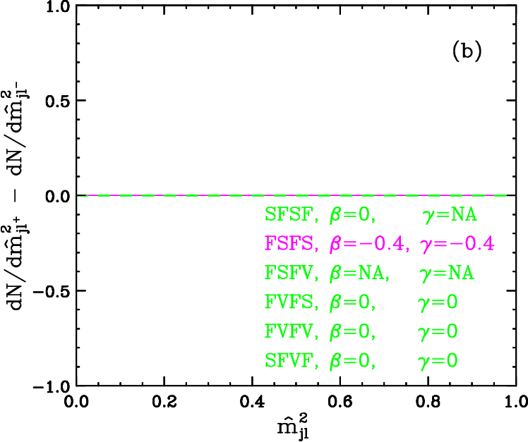


5.1 SFSF example ()
For the SPS1a parameters (155-157) (or alternatively, (162)), eqs. (108-110) predict the following observable invariant mass distributions for the SFSF model:
| (163) | |||||
These distributions are shown with solid (magenta) lines in Figs. 4(a), 5(a) and 6(a), respectively. Following our procedure described above, we first try to fit the dilepton data in Fig. 4(a). Due to the presence of an intermediate scalar particle B, the distribution for the SFSF chain (S=1), is completely flat. However, that does not necessarily mean that the spin of particle B is determined to be zero. In fact, as seen from Fig. 4(a), all other spin configurations except for (SFVF) can also fit this flat distribution, simply by choosing a vanishing parameter. Even the case of (SFVF), whose “best fit” prediction is different from the input data, may still be difficult to discriminate in practice, once we factor in the finite statistics, detector resolution and combinatorial backgrounds. The bad news, therefore, is that we cannot immediately determine the spins from the distribution alone, but the good news is that, as anticipated, we got a measurement of the parameter, which represents some combination of heavy particle couplings and mixing angles.
At this point it is worth comparing our Fig. 4(a) to Fig. 2a in Ref. [21], where a very similar exercise was performed1010 10 Fig. 2a of Ref. [21] is simply the collection of all six solid (magenta) lines in our Fig. 4(a)-(f), i.e. our input “data” for the six different spin configurations, using the same fixed SPS1a values (155-157) for the model dependent parameters.. The two results are quite different, for example we find that 4 out of the 5 “wrong” models can perfectly fit the dilepton “data”, while in Ref. [21] all 6 models give distinct dilepton shapes. Of course, neither of the two results is wrong, and the difference simply arises due to our different philosophy. In Ref. [21] the parameters , and (in our notation) were all kept fixed to the SPS1a values (162), while here we are allowing them to float, since they would not have been measured in advance independently. As a result, we tend to get much more similar distributions, indicating that once we factor in the experimental realism, the actual spin measurements might be even more challenging than previously anticipated.
Having extracted all the relevant information out of the distribution, we now move on to studying the distribution. As we already explained in Sec. 3.2, the advantage of considering as opposed to each one of the individual distributions and is that only depends on exactly the same parameter as the dilepton distribution (see eq. (109)). Since we have just measured by fitting to the data, at this stage there are no free parameters left in the distribution, and it is uniquely predicted for each of the 5 “wrong” spin scenarios. In Fig. 5(a) we plot the resulting predictions for the six spin models, using in each case the corresponding value of , which had been measured in the previous step from the distribution. We see that the distribution can now further differentiate between different spin cases, e.g. it can rule out (in principle) the and (FVFS and FVFV) models. Interestingly, now (SFVF) gives a perfect match, but fortunately, it has already been eliminated from consideration by the analysis of the data at the previous step. Unfortunately, the “wrong” spin scenarios and (FSFS and FSFV) once again give a perfect match to the data, so that even after considering both and , we are still left with 3 distinct possibilities for the spins of the heavy partners. As we shall see later from the other 5 exercises, the SFSF input “data” is somewhat of an unlucky case, since we end up with several spin models which perfectly fit both the and data. More often than not, and by themselves should be sufficient to narrow down the spin configuration alternatives to a single one (or at most two, due to the “twin” spin scenarios discussed in Sec. 4.1).
We are therefore forced to consider our third piece of data, the distribution (110). This distribution does not depend on the previously fitted parameter , and instead needs to be fitted with the other two model-dependent parameters, and . Even though itself does not explicitly depend on , the fit is nevertheless impacted by the measured value of , as the latter determines the allowed range of values for and (see Appendix C for details). The results from our fitting exercise to the SFSF “data” are shown in Fig. 6(a). We see that can now eliminate the remaining two “wrong” spin scenarios and (FSFS and FSFV) and as a result of all three types of fits, we are able to determine uniquely the spin chain as being (SFSF). In addition, we were also able to obtain a measurement of the parameter , which carries information about the couplings and mixing angles of the heavy partners , and . Unfortunately, the parameters and are not experimentally accessible in this case (), since their corresponding basis functions and are identically zero for any (see Appendix B).
Having investigated both the and distributions, we do not need to consider the lepton charge asymmetry , which is simply the ratio of and (see eq. (107)). Numerically the asymmetry and the difference show a very similar pattern of their distributions, and thus provide roughly the same amount of information. However, as we emphasized in Secs. 3.2 and 4.2, there are cases where the asymmetry (as well as ) does not play any role at all. The cases of S=2 (FSFS) and S=3 (FSFV) discussed in the next subsection actually provide such an example.
In the remainder of this section, we shall repeat the exercise that we just went through, each time taking our ‘‘data’’ from a different spin configuration, and trying to fit to it the remaining1111 11 Obviously the “correct” spin configuration will always give a good fit to its own “data”. 5 spin possibilities.
5.2 FSFS and FSFV examples ()
With the SPS1a parameters (162), eqs. (108-110) predict the following observable invariant mass distributions for the FSFS model
| (172) | |||||
| (177) |
which are shown by the solid magenta lines in Figs. 4(b), 5(b), and 6(b), correspondingly.
Similarly, for the FSFV model we get
| (178) | |||||
| (183) |
which are shown with solid magenta lines in Figs. 4(c), 5(c), and 6(c), correspondingly. The distributions (172-177) and (178-183) will be the input sets of data for our next two exercises.
Perhaps the most striking feature in each of the data sets (172-177) and (178-183) is that the distribution, and consequently, the lepton charge asymmetry , are both identically zero. Therefore, they do not convey any information about the spins, since any spin configuration can fit those distributions with the proper choice of parameters as shown in Figs. 6(b) and 6(c). This being the case, we should concentrate on the and distributions.
First we shall discuss the case when the data comes from the FSFS () model, eqs. (172-177). Again, we begin our analysis with , which in this case shows very good discrimination, and can already rule out all of the “wrong” spin combinations. As explained in Sec. 4.1, FSFS () can sometimes be faked by the FSFV (S=3) model, but this could only happen if the parameter in the data satisfies eq. (136), i.e.
| (184) |
Since for SPS1a (see eq. (162)), this condition is not satisfied and the FSFV model cannot fake the FSFS “data”. This is confirmed by our result in Fig. 4(b).
Since the distribution alone already singles out the correct spin configuration, we do not even need to consider the distribution. It is worth pointing out, however, that in this ideal case also can rule out all “wrong” spin models, although the differences are not so pronounced as for , and in reality are likely to be washed out. In summary, the FSFS “data” can be unambiguously interpreted in relation to the spin issue, and we can also get a measurement of the parameter . On the other hand, the parameters and will remain undetermined, since their corresponding basis functions and are identically zero for any (see Appendix B).
Now we shall discuss the case when the data comes from the FSFV () model, eqs. (178-183). This will provide our first example where our spin measurement ends up being inconclusive, yielding two different, equally plausible, possibilities for the spin chain. This result should have already been anticipated, based on our general discussion in Sec. 4.1. There we showed that for any given FSFV data, the FSFS model () can always provide a perfect fit, and furthermore, the value of that would be measured for the “twin” FSFS model is
| (185) |
where we used the SPS1a values for and . Our numerical study explicitly confirms this general expectation as shown in Figs. 4(c), 5(c) and 6(c). In addition, we checked that the distributions for those two “twin” spin models are also identical.
5.3 FVFS and FVFV examples ()
In this subsection we discuss the case of the other “twin” spin pair from Sec. 4.1, namely and (FVFS and FVFV). Using the SPS1a values for the model-dependent parameters, we obtain the following distributions for the FVFS case
| (186) | |||||
which are shown with the solid (magenta) lines in Figs. 4(d), 5(d), and 6(d), correspondingly.
For the FVFV case we get
| (197) | |||||
and those are shown by the solid (magenta) lines in Figs. 4(e), 5(e) and 6(e).
The end result of the two exercises is very similar to what we obtained in the previous subsection for the other “twin” model pair (FSFS and FSFV). It could have also been anticipated from our general discussion in Sec. 4.1. When going in the forward direction, i.e. starting with the FVFS “data” and fitting to it the other 5 models, we do not encounter any spin ambiguities. As already determined in the previous subsection, this is because the SPS1a value of the parameter () does not satisfy the necessary condition (147) for an FVFV model to fake the FVFS data. As a result, the two and distributions are already sufficient to pin down the spin case scenario, and the distribution can then be used as a cross-check and for a measurement of the and parameters.
However, when going in the reverse direction, i.e. starting with the FVFV “data” and fitting the other 5 models including FVFS to it, we do encounter a spin ambiguity, just like in the exercise above. Again, the reason for this was already explained in Sec. 4.1. In agreement with our analytical results, Figs. 4(e), 5(e) and 6(e) show that the FVFS model provides an identical match to the FVFV “data” for all three observable distributions , and . The good news, however, is that while we are left with a two-fold ambiguity with respect to the spins, for each spin scenario the parameters , and are precisely measured, so that we have independent measurements of three different combinations of the heavy partner couplings and mixing angles. In Sec. 5.5 below we shall show how to interpret those measurements in terms of the more fundamental model parameters , , , , , and .
5.4 SFVF example ()
Our final example is the SFVF spin chain, for which the SPS1a model parameters (162) predict the following observable distributions
| (208) | |||||
shown with solid (magenta) lines in Figs. 4(f), 5(f) and 6(f).
The case of (SFVF) is very special, since in this case the dilepton invariant mass distribution (208) exhibits a characteristic term which is not present for any of the other 5 spin configurations that we are considering. Note that the existence of an term in the dilepton SFVF data is generic, i.e. does not depend on the values of the model-dependent parameters such as . This could be easily understood by realising that the dependence originates from the “phase space” basis function , which enters our general formula (108) for the dilepton distribution without any model-dependent coefficients. More generally, an inspection of Table 8 reveals that the dilepton invariant mass distribution is in general given by some polynomial in terms of , whose power is equal to twice the spin of the intermediate particle .1212 12 A similar statement can be made about the invariant mass distributions from Table 9, relating the power of the to the spin of the intermediate C particle. Only in the SFVF case (=6) do we have a spin 1 intermediate particle which brings about an term in . If the presence of this term can be observed in the dilepton data, it would unambiguously1313 13 This observation is subject to our assumption that we do not consider heavy particles of spin 3/2 or higher. In general, an dependence would imply that the spin of the mediating particle is at least 1. signal the presence of a spin 1 mediator. Of course, the size of the coefficient of the term depends on the mass spectrum in the model, but it cannot be vanishingly small – this would require either or , which would correspondingly close off the or the decay, and the whole decay chain will become unobservable. One of our general conclusions, therefore, is that the SFVF model1414 14 Or more generally, a spin 1 or higher intermediate particle., if it exists, should be discernible from the dilepton data alone. Our numerical results in Fig. 4(f) confirm this conclusion – we see that none of the other five models can reproduce the SFVF dilepton data, due to the presence of the term. Pictorially this can be seen from the fact that the predictions of the models in Fig. 4 are always straight lines, while for the model (SFVF) the prediction is never a straight line, due to the higher order dependence.
| Result from | Data originating from model | Total No. | |||||
| fitting to | SFSF | FSFS | FSFV | FVFS | FVFV | SFVF | of fakes |
| only | 5 | 1 | 3 | 2 | 4 | 1 | 10 |
| only | 4 | 1 | 4 | 1 | 2 | 2 | 8 |
| only | 1 | 6 | 6 | 1 | 3 | 1 | 12 |
| 3 | 1 | 2 | 1 | 2 | 1 | 4 | |
| 1 | 1 | 3 | 1 | 2 | 1 | 3 | |
| 1 | 1 | 4 | 1 | 2 | 1 | 4 | |
| 1 | 1 | 2 | 1 | 2 | 1 | 2 | |
Before we move on to the next subsection, where we shall interpret our measurements of the , and parameters, we briefly summarise the results from the preceding six exercises in Table 3. The table shows the number of different spin configurations from Table 1 which can fit perfectly a given data set (, , , or some combination thereof). Since this number depends on the spin configuration of the input “data”, we show 6 different columns, one for each different spin configuration of the “data”. The last column lists the total number of “wrong” spin configurations allowed by the corresponding data set in all 6 exercises. This number was obtained simply by summing all the entries from the preceding 6 columns and subtracting 6 to exclude the correct configurations among them.
While one should be mindful that the number counts exhibited in Table 3 are only valid for the SPS1a parameter choice, there are still some interesting conclusions which can be drawn from it. For example, we do not notice any particular pattern in the horizontal direction. In particular, the discriminating power of the different data sets, say , and , varies greatly from model to model. There are cases where a single distribution works very well, for example for FSFS and SFVF, for FSFS and FVFS and for SFSF, FVFS and SFVF. In all those cases the spin configuration is uniquely fixed by studying a single distribution! On the other hand, there are also cases where each one of these individual distributions performs rather poorly, for example for SFSF, for SFSF and FSFV and for FSFS and FSFV. In the end, each one of the , and distributions, when considered in isolation, yields on the order of 10 fake spin configurations. What this simply means is that no single distribution can be universally “better” than the others.
Things begin to get more interesting when we start combining information gained from 2 or more different distributions. For example, when we combine any 2 out of our three observable distributions , and , the total number of fake solutions drops down to 3 or 4. Now again, which particular pair works better, is a model-dependent issue: fails for the SFSF model, while and both fail for the FSFV model. Finally, combining the information from all three distributions, , we narrow down the remaining spin choices even further, but as we saw in Secs. 5.2 and 5.3, there are still two cases of exact duplication, which are nothing but the “twin” spin scenarios of Sec. 4.1. Since this duplication is due to an exact mathematical identity, it will obviously still persist if we were to repeat our analysis including all the experimental realism (backgrounds, resolution, combinatorics, etc.). In fact, due to the expected imperfections in the real data, one may get even more duplicate examples, if anything.
5.5 Measurements of couplings and mixing angles
| Spin | Parameters measured from distribution | |||
|---|---|---|---|---|
| chain | ||||
| SFSF | ||||
| FSFS | ||||
| FSFV | ||||
| FVFS | ||||
| FVFV | ||||
| SFVF | ||||
Recall that our general method from Sec. 4 yields not only a determination of a possible spin chain fitting the data, but also a measurement of the model-dependent , and parameters from eqs. (111-113). Even in the spin duplication scenarios found in Secs. 5.2 and 5.3, we still have a certain measurement of the , and coefficients for each of the two allowed spin chains. This is illustrated in Table 4 where we summarize the available measurements of the , and parameters in each individual spin case. Notice that only in the last three spin cases (FVFS, FVFV and SFVF) we are able to measure the complete set of all three parameters , and . In contrast, for the SFSF model chain we can only determine , while and remain unknown. On the other hand, for the FSFS and FSFV chains we can only determine , while and remain arbitrary. In the remainder of this section we shall discuss the interpretation of those measurements in terms of the couplings and mixing angles of the heavy partners, i.e. we shall relate the measured values of and/or and/or to the underlying model parameters , , and .
First, let us consider the case where we determine a spin chain to be one of the following three: FVFS, FVFV or SFVF. Then, as seen from Table 4, we will be able to measure the values of all three parameters , and . If we have correctly determined the spin chain, these values will be simply the starting SPS1a inputs (162). Substituting those in eqs. (119-124), we obtain the two sets of solutions discussed at the beginning of Section 4:
| (218) |
and
| (219) |
where the first (second) solution corresponds to choosing the upper (lower) sign in eqs. (119-124). As expected, we obtain that each set is a one-parameter family of solutions, parameterised by the value of the particle-antiparticle ratio . The first solution set (218) reproduces the SPS1a parameter set for , but of course, we would have no way of knowing that is the correct value of , since we would have to measure independently by some other means. However, notice that even though we do not know the exact value of at this point, the solutions (218-219) unambiguously restrict the allowed range for from (126) to be
| (220) |
which is by itself already an important and useful experimental determination.
Now let us discuss more specifically the case where the data is due to an FVFS or an FVFV spin chain ( or ). As already explained in Sec. 4.1 and explicitly seen in our examples in Sec. 5.3, here we may encounter a second solution for the spin chain, with its own measured , and parameters. We remind the reader that when the data comes from an FVFV chain, there is always a duplicate spin solution due to an FVFS chain, while if the data comes from an FVFS chain, the duplicate FVFV solution exists only if the conditions (147, 148) are satisfied. While the duplicate spin chain prevents us from uniquely resolving the spin question, the interpretation of its , and parameters can be done in a very similar fashion. Consider our duplication example from Sec. 5.3 where an FVFS () spin chain was able to “fake” the FVFV () data. All three parameters , and were still uniquely measured but the obtained values were not the starting SPS1a values. Instead, our fitting procedure found
| (221) |
as shown in Fig. 4(e), 5(e) and 6(e). We see that the parameter for the twin spin chain was found to be the same as the true parameter of the data (), while both the and parameters of the twin spin case are a factor of 20 smaller than the original inputs (162). This fact can be easily understood from our general results from Sec. 4.1 – the conditions (147, 148) which guarantee the existence of a duplicate solution, relate the values of and for the two spin chains, and by the same factor of , where we have used the SPS1a value of . Just as before, the measurements (221) translate into a measurement of the effective couplings and mixing angles as a function of , up to a two-fold ambiguity. Substituting (221) in eqs. (119-124), we obtain the two solutions
| (222) |
or
| (223) |
As expected, these solutions exhibit the same symmetry (118) as the solutions (218) and (219) for the “correct” spin configuration. Comparing eqs. (222, 223) to eqs. (218, 219), we see that we obtain the same result for the , , and couplings! In other words, although it may not be clear what is the correct spin chain – FVFS or FVFV, the chirality of the couplings at the quark and at the near lepton vertex will be known (up to the inescapable two-fold ambiguity due to (118)). This can be simply understood by noticing from eqs. (121-124) that the couplings , , and only depend on and through their ratio, which is the same for the correct and the fake spin solution, since and are scaled by the same factor (see eqs. (141,143). Just as before, for the “wrong” spin chain we also obtain a constraint on the allowed range of the particle-antiparticle fraction at the LHC:
| (224) |
Notice that this is identical to the result (220) for the “correct” spin chain, so that the experimental determination of the range of the parameter also does not suffer from the duplicate spin ambiguity.
This concludes our discussion of the spin cases where we can measure all three parameters , and . For the remaining three spin chains, only partial information will be available (see Table 4). For example, in case of SFSF we can only measure the parameter, which gives us one relation among and
| (225) |
or alternatively, among , and :
| (226) |
Unfortunately, we are unable to pin down further the precise values of , and , and furthermore, remains completely unknown.
Similarly, in case of FSFS and FSFV, we can measure the parameter, which gives us a relation between and :
| (227) |
Normally, we would not be able to go any further, but the SPS1a parameter set is “lucky” in the sense that it yields one of the two extreme values of (see Fig. 3). In those circumstances, we can determine the actual values of and , and subsequently, , , and , up to the usual ambiguity:
| (228) |
or
| (229) |
Unfortunately, in either case, , and will remain unconstrained.
Finally, we briefly comment on the possibility of spin duplication between FSFS and FSFV discussed in Sec. 4.1 and Sec. 5.2. Here we will also obtain a measurement of the parameter for the “wrong” spin chain. The two parameters (for the “wrong” and for the “correct” spin configurations) are related according to (132) and the analysis for the couplings in the case of the “wrong” spin chain can be done in complete analogy.
6 Summary and conclusions
We conclude by summarizing the main steps of our method for measuring spins, couplings and mixing angles of heavy partners in cascade decays with missing energy. We shall then contrast it to other proposals for spin measurements in the literature.
The method involves the following basic steps.
- 1.
Data preparation. Identify a decay chain of interest which would yield three observable SM fermions. (In this paper we considered the example of a quark jet followed by two leptons, which is commonly encountered in models of supersymmetry and extra dimensions.) Then form the three observable invariant mass distributions for each pair of well-defined objects: , and . In order to remove the combinatorial ambiguities, perform an opposite-flavor subtraction on the leptons and a mixed-event subtraction on the jet. Apply final cuts to possibly suppress any SM and new physics backgrounds. As the end product from this step one obtains the three ditributions , and defined in eqs. (108-110).
- 2.
Mass measurements. This step is optional, since the mass measurements can in principle be performed simultaneously with the spin fits described below. However, in practice we expect that the invariant mass distributions would reveal their kinematic endpoints rather early on, so that the mass spectrum can be measured in advance of the spin determination. At the end of this step one would know the mass spectrum, i.e. the values of , and which enter the functions , as well as the kinematic endpoints which unit normalise our invariant mass variables (see eqs. (12) and (81)).
- 3.
Spin measurements. This step represents the actual spin measurement. One tries to fit1515 15 In general, those are three-parameter fits for the floating, a priori unknown, coefficients , and . However, as discussed in Sec. 4 and illustrated with our numerical examples in Sec. 5, one could make use of the fact that the and distributions only depend on the parameter . Thus one could first extract from and/or , and then use this value to fit for and , as shown in Appendix C. the data for the , and distributions obtained in Step 1 with the theoretical predictions (108-110), for each value of , i.e. for each set of allowed spin configurations for particles , , and (see Table 1). If the fit is good, that particular spin chain is ruled in, while if the fit is bad, that particular spin chain will be ruled out. Our expectations for the generic outcome of this exercise are summarised in Table 5. When using the data from all three distributions , and , we expect that the fits will be able to rule out all but the correct spin configuration. The only exceptions are the spin duplication cases discussed in Sec. 4.1, when one may end up with at most two spin chain alternatives.
- 4.
Measurements of couplings and mixing angles. In this step one uses any available best-fit values for , and obtained in the previous step, and determines the couplings , , , , and from eqs. (119-124). There will be two different solutions due to the symmetry, as discussed in Sec. 4 and illustrated with some examples in Sec. 5.5. In addition, eq. (126) provides a restriction on the allowed range of values for the particle-antiparticle fraction at the LHC.
| Data | Can this data be fitted by model | |||||
|---|---|---|---|---|---|---|
| from | SFSF | FSFS | FSFV | FVFS | FVFV | SFVF |
| SFSF | yes | no | no | no | no | no |
| FSFS | no | yes | maybe | no | no | no |
| FSFV | no | yes | yes | no | no | no |
| FVFS | no | no | no | yes | maybe | no |
| FVFV | no | no | no | yes | yes | no |
| SFVF | no | no | no | no | no | yes |
Having summarised the main steps of our method, we are ready to compare it to other approaches for spin measurements which already exist in the literature. In principle, no single method is universally applicable, therefore the availability of different and complementary techniques is an important virtue. Which method ends up being most successful in practice, will depend on the specific new physics scenario that we may encounter. With those caveats, we should point out some features of our method which are likely to make it relevant and successful, if a missing energy signal of new physics is seen at the LHC and/or the Tevatron.
- •
Many of the existing techniques for spin determinations (see, for example, [30, 31, 45, 46]) have been originally developed in the context of lepton colliders, where the total center of mass energy in each event is known. Consequently, at hadron colliders, those methods are applicable only if the events can be fully reconstructed. In new physics scenarios with dark matter WIMPs, this appears to be rather challenging, since there are two invisible WIMP particles escaping the detector. In some special circumstances, where two sufficiently long decay chains can be identified in the event, full reconstruction might be possible [10, 11, 12], but in any case, this appears to require very large data samples. In contrast, our method relies on invariant mass distributions, which are frame-independent, and we do not need to have the event fully reconstructed. Furthermore, the event reconstruction techniques currently being discussed rely on the pair-production of two heavy particles, both of which decay visibly to the lightest WIMP. Our method, on the other hand, does not require the presence of two separate decay chains in the event, and can be in principle also applied to the associated production of a WIMP with only one other heavy partner.
- •
The invariant mass distributions , and that we propose to analyse, are the basic starting point for any precision study of new physics parameters. In the past they have been extensively discussed in relation to mass measurements, and we now simply propose to fully analyse them for the encoded spin information as well.
- •
One major advantage of our method in comparison to various event counting techniques [33, 35, 44, 47] is that we do not need to know anything about a number of additional and a priori also unknown quantities such as the production cross-sections for the different parton-level initial states, the branching fractions, the experimental efficiencies, etc. Indeed, our method in essence only uses unit-normalised distributions, and is not affected by any of these additional variables.
- •
The previous three advantages are common to all studies which have relied exclusively on invariant mass distributions for spin determinations [19, 20, 21, 22, 32, 36, 37, 38, 39, 40, 41, 42, 43]. In comparison to those works, the main advantage of our approach is that it is completely general and model-independent, in particular we make no a priori assumptions about the type of couplings in each vertex of Fig. 1, or about the particle-antiparticle fraction . As a result, we were actually able to come up with measurements of certain combinations of those couplings and the parameter (see Secs. 4 and 5.5).
In conclusion, we reiterate that our goal in this paper was simply to present the basic idea of our method, and demonstrate that it can work as a matter of principle. Therefore in our analysis in Sec. 5 we did not include any realistic detector simulation, backgrounds (SM and combinatorial) etc. All of these factors will be investigated in a future publication [18].
Acknowledgments.
This work is supported in part by a US Department of Energy grant DE-FG02-97ER41029. Fermilab is operated by Fermi Research Alliance, LLC under Contract No. DE-AC02-07CH11359 with the U.S. Department of Energy.Appendix A Appendix: The basis functions
The basis functions are listed in Table 6 and the basis functions are given in Table 7. Below we explicitly show the remaining basis functions :
SFSF ()
FSFS ()
FSFV ()
FVFS ()
FVFV ()
SFVF ()
| Spins | |||
|---|---|---|---|
| 1 | |||
| 2 | |||
| 3 | |||
| 4 | |||
| 5 | |||
| 6 |
| Spins | |||
|---|---|---|---|
| 1 | |||
| 2 | |||
| 3 | |||
| 4 | |||
| 5 | |||
| 6 |
Appendix B Appendix: The basis functions , , and
The basis functions , , and are listed in Table 8. The basis functions , , and are given in Table 9. Below we explicitly show the remaining basis functions , , and :
SFSF ()
| (B.1) | |||||
FSFS ()
| (B.14) | |||||
FSFV ()
| (B.23) | |||||
FVFS ()
FVFV ()
SFVF ()
| Spins | |||||
|---|---|---|---|---|---|
| 1 | |||||
| 2 | |||||
| 3 | |||||
| 4 | |||||
| 5 | |||||
| 6 |
| Spins | |||||
|---|---|---|---|---|---|
| 1 | |||||
| 2 | |||||
| 3 | |||||
| 4 | |||||
| 5 | |||||
| 6 |
Appendix C Appendix: Fitting procedure for the parameters , and
In the absence of any error bars, we use a rather naive matching criterion, namely
| (C.1) |
where represents the experimental data that needs to be fitted and is the theoretical prediction for it. We then minimize the function for , and/or , as appropriate. , and are fixed constant values of the , and parameters as predicted for the corresponding study point. A more sophisticated analysis including the expected statistical uncertainties is postponed for a future publication [18].


As we discussed in Sec. 4, fitting to the or to the distribution is a simple one-parameter fit for , while fitting to the data is a two-parameter fit for and . Fig. 7 shows sample results from our fits for and performed in the course of the exercises described in Sec. 5. In each plot in Fig. 7, the “data” comes from the first spin chain (shown in red) at the top of each plot, which is then fitted with the distribution predicted by the second spin chain (shown in blue). The contour lines represent constant values of , where has already been fixed by fitting to . The blue dot corresponds to the absolute minimum of , ignoring any restrictions on , and . However, the parameters , and are not completely independent from each other. For any given , the physically allowed region in the parameter space is described by an envelope which satisfies
| (C.2) | |||
| (C.3) | |||
| (C.4) | |||
| (C.5) |
In Fig. 7 we denote this allowed region in white (sometimes it may reduce to a single line). The green triangle corresponds to the minimum of the function within this restricted parameter set. The green triangle solution for and was then used for our plots in Fig. 6. For the two cases with FVFV (S=5) “data”, the global minimum happens to lie within the (white) allowed region and so the blue dot and the green triangle coincide.
For the extreme values of , the (white) allowed region collapses to one or two lines:
| (C.6) | |||||
| (C.7) |
References
- [1] For a recent review, see G. Bertone, D. Hooper and J. Silk, “Particle dark matter: Evidence, candidates and constraints,” Phys. Rept. 405, 279 (2005) [arXiv:hep-ph/0404175].
- [2] See, for example, J. Hubisz, J. Lykken, M. Pierini and M. Spiropulu, “Missing energy look-alikes with 100 pb-1 at the LHC,” arXiv:0805.2398 [hep-ph], and references therein.
- [3] For a review, see G. Jungman, M. Kamionkowski and K. Griest, “Supersymmetric dark matter,” Phys. Rept. 267, 195 (1996) [arXiv:hep-ph/9506380].
- [4] For a review, see D. Hooper and S. Profumo, “Dark matter and collider phenomenology of universal extra dimensions,” Phys. Rept. 453, 29 (2007) [arXiv:hep-ph/0701197].
- [5] H. C. Cheng and I. Low, “TeV symmetry and the little hierarchy problem,” JHEP 0309, 051 (2003) [arXiv:hep-ph/0308199].
- [6] A. Birkedal, A. Noble, M. Perelstein and A. Spray, “Little Higgs dark matter,” Phys. Rev. D 74, 035002 (2006) [arXiv:hep-ph/0603077].
- [7] T. Hur, H. S. Lee and S. Nasri, “A Supersymmetric U(1)’ Model with Multiple Dark Matters,” Phys. Rev. D 77, 015008 (2008) [arXiv:0710.2653 [hep-ph]].
- [8] H. S. Lee, “Lightest U-parity Particle (LUP) dark matter,” Phys. Lett. B 663, 255 (2008) [arXiv:0802.0506 [hep-ph]].
- [9] A. Birkedal, K. Matchev and M. Perelstein, “Dark matter at colliders: A model-independent approach,” Phys. Rev. D 70, 077701 (2004) [arXiv:hep-ph/0403004].
- [10] H. C. Cheng, J. F. Gunion, Z. Han, G. Marandella and B. McElrath, “Mass Determination in SUSY-like Events with Missing Energy,” JHEP 0712, 076 (2007) [arXiv:0707.0030 [hep-ph]].
- [11] M. M. Nojiri, G. Polesello and D. R. Tovey, “A hybrid method for determining SUSY particle masses at the LHC with fully identified cascade decays,” JHEP 0805, 014 (2008) [arXiv:0712.2718 [hep-ph]].
- [12] H. C. Cheng, D. Engelhardt, J. F. Gunion, Z. Han and B. McElrath, “Accurate Mass Determinations in Decay Chains with Missing Energy,” arXiv:0802.4290 [hep-ph].
- [13] I. Hinchliffe, F. E. Paige, M. D. Shapiro, J. Soderqvist and W. Yao, “Precision SUSY measurements at LHC,” Phys. Rev. D 55, 5520 (1997) [arXiv:hep-ph/9610544].
- [14] B. C. Allanach, C. G. Lester, M. A. Parker and B. R. Webber, “Measuring sparticle masses in non-universal string inspired models at the LHC,” JHEP 0009, 004 (2000) [arXiv:hep-ph/0007009].
- [15] B. K. Gjelsten, D. J. Miller and P. Osland, “Measurement of SUSY masses via cascade decays for SPS 1a,” JHEP 0412, 003 (2004) [arXiv:hep-ph/0410303].
- [16] B. K. Gjelsten, D. J. Miller and P. Osland, “Measurement of the gluino mass via cascade decays for SPS 1a,” JHEP 0506, 015 (2005) [arXiv:hep-ph/0501033].
- [17] D. J. Miller, P. Osland and A. R. Raklev, “Invariant mass distributions in cascade decays,” JHEP 0603, 034 (2006) [arXiv:hep-ph/0510356].
- [18] M. Burns, K. Kong, K. Matchev and M. Park, in preparation.
- [19] A. J. Barr, “Using lepton charge asymmetry to investigate the spin of supersymmetric particles at the LHC,” Phys. Lett. B 596, 205 (2004) [arXiv:hep-ph/0405052].
- [20] J. M. Smillie and B. R. Webber, “Distinguishing spins in supersymmetric and universal extra dimension models at the Large Hadron Collider,” JHEP 0510, 069 (2005) [arXiv:hep-ph/0507170].
- [21] C. Athanasiou, C. G. Lester, J. M. Smillie and B. R. Webber, “Distinguishing spins in decay chains at the Large Hadron Collider,” JHEP 0608, 055 (2006) [arXiv:hep-ph/0605286].
- [22] C. Athanasiou, C. G. Lester, J. M. Smillie and B. R. Webber, “Addendum to ’Distinguishing spins in decay chains at the Large Hadron Collider’,” arXiv:hep-ph/0606212.
- [23] J. A. Bagger, K. T. Matchev, D. M. Pierce and R. j. Zhang, “Weak-scale phenomenology in models with gauge-mediated supersymmetry breaking,” Phys. Rev. D 55, 3188 (1997) [arXiv:hep-ph/9609444].
- [24] T. Gherghetta, G. F. Giudice and J. D. Wells, “Phenomenological consequences of supersymmetry with anomaly-induced masses,” Nucl. Phys. B 559, 27 (1999) [arXiv:hep-ph/9904378].
- [25] J. L. Feng and T. Moroi, “Supernatural supersymmetry: Phenomenological implications of anomaly-mediated supersymmetry breaking,” Phys. Rev. D 61, 095004 (2000) [arXiv:hep-ph/9907319].
- [26] M. Schmaltz and W. Skiba, “Minimal gaugino mediation,” Phys. Rev. D 62, 095005 (2000) [arXiv:hep-ph/0001172].
- [27] H. C. Cheng, K. T. Matchev and M. Schmaltz, “Radiative corrections to Kaluza-Klein masses,” Phys. Rev. D 66, 036005 (2002) [arXiv:hep-ph/0204342].
- [28] H. C. Cheng, K. T. Matchev and M. Schmaltz, “Bosonic supersymmetry? Getting fooled at the LHC,” Phys. Rev. D 66, 056006 (2002) [arXiv:hep-ph/0205314].
- [29] H. C. Cheng, I. Low and L. T. Wang, “Top partners in little Higgs theories with T-parity,” Phys. Rev. D 74, 055001 (2006) [arXiv:hep-ph/0510225].
- [30] M. Battaglia, A. Datta, A. De Roeck, K. Kong and K. T. Matchev, “Contrasting supersymmetry and universal extra dimensions at the CLIC multi-TeV e+ e- collider,” JHEP 0507, 033 (2005) [arXiv:hep-ph/0502041].
- [31] M. Battaglia, A. K. Datta, A. De Roeck, K. Kong and K. T. Matchev, “Contrasting supersymmetry and universal extra dimensions at colliders,” In the Proceedings of 2005 International Linear Collider Workshop (LCWS 2005), Stanford, California, 18-22 Mar 2005, pp 0302 [arXiv:hep-ph/0507284].
- [32] A. Datta, K. Kong and K. T. Matchev, “Discrimination of supersymmetry and universal extra dimensions at hadron colliders,” Phys. Rev. D 72, 096006 (2005) [Erratum-ibid. D 72, 119901 (2005)] [arXiv:hep-ph/0509246].
- [33] A. Datta, G. L. Kane and M. Toharia, “Is it SUSY?,” arXiv:hep-ph/0510204.
- [34] A. J. Barr, “Measuring slepton spin at the LHC,” JHEP 0602, 042 (2006) [arXiv:hep-ph/0511115].
- [35] P. Meade and M. Reece, “Top partners at the LHC: Spin and mass measurement,” Phys. Rev. D 74, 015010 (2006) [arXiv:hep-ph/0601124].
- [36] A. Alves, O. Eboli and T. Plehn, “It’s a gluino,” Phys. Rev. D 74, 095010 (2006) [arXiv:hep-ph/0605067].
- [37] L. T. Wang and I. Yavin, “Spin Measurements in Cascade Decays at the LHC,” JHEP 0704, 032 (2007) [arXiv:hep-ph/0605296].
- [38] S. Abdullin et al. [TeV4LHC Working Group], “Tevatron-for-LHC report: Preparations for discoveries,” arXiv:hep-ph/0608322.
- [39] J. M. Smillie, “Spin Correlations in Decay Chains Involving W Bosons,” Eur. Phys. J. C 51, 933 (2007) [arXiv:hep-ph/0609296].
- [40] K. Kong and K. T. Matchev, “Phenomenology of universal extra dimensions,” AIP Conf. Proc. 903, 451 (2007) [arXiv:hep-ph/0610057].
- [41] C. Kilic, L. T. Wang and I. Yavin, “On the Existence of Angular Correlations in Decays with Heavy Matter Partners,” JHEP 0705, 052 (2007) [arXiv:hep-ph/0703085].
- [42] A. Alves and O. Eboli, “Unravelling the sbottom spin at the CERN LHC,” Phys. Rev. D 75, 115013 (2007) [arXiv:0704.0254 [hep-ph]].
- [43] C. Csaki, J. Heinonen and M. Perelstein, “Testing Gluino Spin with Three-Body Decays,” JHEP 0710, 107 (2007) [arXiv:0707.0014 [hep-ph]].
- [44] A. Datta, P. Dey, S. K. Gupta, B. Mukhopadhyaya and A. Nyffeler, “Distinguishing the Littlest Higgs model with T-parity from supersymmetry at the LHC using trileptons,” Phys. Lett. B 659, 308 (2008) [arXiv:0708.1912 [hep-ph]].
- [45] M. R. Buckley, H. Murayama, W. Klemm and V. Rentala, “Discriminating spin through quantum interference,” arXiv:0711.0364 [hep-ph].
- [46] M. R. Buckley, B. Heinemann, W. Klemm and H. Murayama, “Quantum Interference Effects Among Helicities at LEP-II and Tevatron,” Phys. Rev. D 77, 113017 (2008) [arXiv:0804.0476 [hep-ph]].
- [47] G. L. Kane, A. A. Petrov, J. Shao and L. T. Wang, “Initial determination of the spins of the gluino and squarks at LHC,” arXiv:0805.1397 [hep-ph].
- [48] T. Appelquist, H. C. Cheng and B. A. Dobrescu, “Bounds on universal extra dimensions,” Phys. Rev. D 64, 035002 (2001) [arXiv:hep-ph/0012100].
- [49] B. A. Dobrescu, K. Kong and R. Mahbubani, “Leptons and photons at the LHC: Cascades through spinless adjoints,” JHEP 0707, 006 (2007) [arXiv:hep-ph/0703231].
- [50] N. Ozturk [ATLAS Collaboration], “SUSY Parameters Determination with ATLAS,” arXiv:0710.4546 [hep-ph].
- [51] A. Birkedal, R. C. Group and K. Matchev, “Slepton mass measurements at the LHC,” In the Proceedings of 2005 International Linear Collider Workshop (LCWS 2005), Stanford, California, 18-22 Mar 2005, pp 0210 [arXiv:hep-ph/0507002].
- [52] B. K. Gjelsten, D. J. Miller, P. Osland and A. R. Raklev, “Mass determination in cascade decays using shape formulas,” AIP Conf. Proc. 903, 257 (2007) [arXiv:hep-ph/0611259].
- [53] K. Kong and K. Matchev, in preparation.