Rigidity and uniruling for Lagrangian submanifoldsThanks: The first author was partially supported by the ISRAEL SCIENCE FOUNDATION (grant No. 1227/06 *); the second author was supported by an NSERC Discovery grant and a FQRNT Group Research grant
1. Introduction
The purpose of this paper is to explore the topology of monotone Lagrangian submanifolds inside a symplectic manifold by exploiting the relationships between the quantum homology of and various quantum structures associated to the Lagrangian . We show that the class of monotone Lagrangians satisfies a number of structural rigidity properties which are particularly strong when the ambient symplectic manifold contains enough genus-zero pseudo-holomorphic curves. Indeed, we will see that (very often) if is “highly” uniruled by curves of area , then (or just ) is uniruled by curves of area strictly smaller than (see 1.1.2 for the definition of the appropriate notions of uniruling).
1.1. Setting
All our symplectic manifolds will be implicitly assumed to be connected and tame (see [ALP]). The main examples of such manifolds are closed symplectic manifolds, manifolds which are symplectically convex at infinity as well as products of such. All the Lagrangians submanifolds will be assumed to be connected and closed (i.e. compact, without boundary).
We start by emphasizing that our results apply to monotone Lagrangians. These are characterized by the fact that the morphisms:
the first given by integration and the second by the Maslov index, are proportional with a positive proportionality constant with . Moreover, we will include here in the definition of the monotonicity the assumption that the minimal Maslov index,
of a homotopy class of strictly positive Maslov index is at least two, . If is monotone, then is also monotone and divides where is the minimal Chern number of
1.1.1. Size of Lagrangians
Fix a Lagrangian submanifold .
We say that a symplectic embedding of the closed, standard symplectic ball of radius , , is relative to if
These types of embedding were first introduced and used in [BC2] and [BC1].
Consider now a vector . We will not allow for both and to vanish. If just one does, say , we will use the notation .
Definition 1.1.1.
The mixed symplectic packing number, , of type of is defined by:
where the supremum is taken over all such that there are mutually disjoint symplectic embeddings
so that the ’s are embeddings relative to .
The most widespread example of such vectors have all their components equal to . We also notice that is the well-known Gromov width of : the supremum of over all symplectic embeddings of into . A similar notion has been introduced in [BC1], see also [CL2], to “measure” Lagrangians: the width of a Lagrangian, , is the supremum of over all symplectic embeddings of which are relative to . With our conventions, . Moreover, , the Gromov width of the complement of , is given by .
1.1.2. Uniruling
The main technique used to prove width and packing estimates is based on establishing uniruling results.
Definition 1.1.2.
We say that is uniruled of type and order (or shorter, is - uniruled of order ) if for any distinct points , and any distinct points, , there exists a Baire second category (generic) family of almost complex structures with the property that for each there exists a non-constant -holomorphic disk so that , , and . In case is void, we take , and instead of a disk, is required to be a non-constant -holomorphic sphere so that .
If is -uniruled we will say that is uniruled of type . Thus the usual notion of uniruling for a symplectic manifold - is uniruled if through each point of passes a -sphere in some fixed homotopy class in - is equivalent in our terminology with being -uniruled. Similarly, in case is - uniruled we will say that is -uniruled. Additionally, if we say that is uniruled.
The relation with packing is given by the following fact:
Lemma 1.1.3.
If the pair is - uniruled of order , then for any vector the mixed symplectic packing number verifies:
where is the monotonicity constant, .
The proof of this is standard and is a small modification of an argument of Gromov [Gro]. It comes down to the following simple remark which also explains the factor in the definition of . If a -curve with boundary on a Lagrangian goes through the center of a standard symplectic ball or radius embedded in relative to so that coincides with the standard almost complex structure inside the ball, then we have . This is in contrast to the case when has no boundary, when the inequality is, as is well-known, .
The simplest way to detect algebraically that is -uniruled is to find some class and so that, for distinct points , and a generic , the evaluation at distinct points on the -spheres of class which pass through the fixed points , has a homologically non-trivial image in the product . This can be translated in terms of Gromov-Witten invariants: if there exist and classes , so that
| (1) |
where the class of the point, , appears times, then is clearly -uniruled (we recall that the Gromov-Witten invariant counts - in this paper with coefficients - the number of -spheres in the homotopy class which each pass through generic cycles representing the homology classes ).
Remark 1.1.4.
If we fix and add the requirement that , then, by the splitting property of Gromov-Witten invariants, the uniruling condition implies for some choices of and . Of course, this can be re-interpreted in quantum homology as the relation where represents the point, is the fundamental class, and the Novikov ring used is .
A stronger condition will play a key role in the following. Consider the quantum homology of with coefficients in with (where is the minimal Chern number). This is .
Definition 1.1.5.
With the notation above we say that is point invertible if is invertible in . This implies that there exists , , and so that, if we put , then in we have
The natural number above is uniquely defined and we specify it by saying that is point invertible of order .
Of course, as indicated above, a point-invertible manifold is -uniruled. The class of point invertible manifolds includes, for example, and the quadric . Moreover, in view of the product formula for Gromov-Witten invariants, this class is closed with respect to products.
In general, no such direct algebraic criteria can be found to test the existence of mixed uniruling of the pair or even whether itself is uniruled because relative Gromov-Witten invariants are not well-defined in full generality.
1.2. Main results
Recall that by the work of Oh [Oh2] if is a monotone Lagrangian - which we will assume from now on, then the Floer homology with -coefficients is well-defined (the construction will be briefly recalled later in the paper). Floer homology is easily seen to be isomorphic (in general not canonically) to a quotient of a sub-vector space of . Here is singular homology and where the degree of is (see §3.2 g for the precise definition). Thus, there are two extremal cases:
Definition 1.2.1.
If we say that is narrow; if there exists an isomorphism , then we call wide. Note that the latter isomorphism is not required to be canonical in any sense.
Remarkably, all known monotone Lagrangians are either narrow or wide. We will see that the dichotomy narrow - wide plays a key role in structuring the properties of monotone Lagrangians. In particular, narrow Lagrangians tend to be small in the sense that their width is bounded and non-narrow ones tend to be barriers in the sense of [Bir1]: the width of their complement tends to be smaller than that of the ambient manifold. Wide Lagrangians are even more rigid.
1.2.1. Geometric rigidity.
We start with one result concerning narrow Lagrangians which also shows that the “narrow - wide” dichotomy holds in a variety of cases (related results are due to Buhovsky [Buh1]):
Theorem 1.2.2.
Let be a monotone Lagrangian. Assume that its singular homology is generated as a ring (with the intersection product) by .
- i.
If , then is either wide or narrow. Moreover, if , then is wide.
- ii.
In case is narrow, then is uniruled of order with if , and if . Moreover, where is the monotonicity constant. In particular, the width of narrow monotone Lagrangians is “universally” bounded: . In case is narrow and not a homology sphere the bound can be improved to .
Note that the finiteness of from point ii is not trivial since is not assumed to be compact nor of finite volume or width. Moreover, when is not narrow, might be infinite. For example, zero-sections in cotangent bundles (which are wide) have infinite width. A class of Lagrangians for which Theorem 1.2.2 gives non-trivial information is that of monotone Lagrangian tori. In this case is generated by hence we can take . As we see that any monotone Lagrangian torus is either narrow or wide. In case such a Lagrangian is narrow we have .
To obtain any meaningful uniruling results for Lagrangians which are not narrow, the same example of zero sections in cotangent bundles shows that some additional conditions need to be imposed on the ambient manifold .
Theorem 1.2.3.
Let be a monotone Lagrangian in a symplectic manifold which is point-invertible of order .
- i.
If is not narrow, then is uniruled of type of order . In particular,
- ii.
If is wide, then is uniruled of order and we have:
(2)
We emphasize that the somewhat surprising part of the statement is that the uniruling involving is of order strictly lower than whenever is point invertible of order precisely (in particular, it might happen that itself is uniruled of order precisely ).
Remark 1.2.4.
- a.
There are a few additional immediate inequalities that are worth mentioning: as is uniruled we have and so . Moreover, as is 2-uniruled, we have . Obviously, we always have .
- b.
These general inequalities do not imply the inequality (2). Indeed, in contrast to , the two balls involved in estimating separately the width of and that of its complement are not required to be disjoint !
- c.
A non-trivial consequence of point i of the Theorem is that if is point-invertible of order and is non-narrow, then .
- d.
Assuming the setting of the point 2 of the Theorem we deduce from the fact that is uniruled of order , that . However, this inequality lacks interest because (since ).
1.2.2. Corollaries for Lagrangians in
We endow with the standard Kähler symplectic structure normalized so that . With this normalization we have hence . Note also that for every monotone Lagrangian we have and that is point invertible of order .
Corollary 1.2.5.
Let be a monotone Lagrangian in .
- i.
At least one of the following inequalities is verified:
- a.
- b.
Moreover, if is not narrow then possibility b holds and in fact we have
- a.
- ii.
If is wide, then we have
In case is not narrow, the inequality follows directly from Theorem 1.2.3. If is narrow, as can not be a homology sphere (see e.g. [BC4]) we can take in Theorem 1.2.2 which then implies the inequality at i a above. Point ii of the Corollary follows from point ii of Theorem 1.2.3.
Corollary 1.2.5 implies in particular that for any monotone Lagrangian in we have
| (3) |
or, in other words, any monotone Lagrangian in is either a barrier (in the sense of [Bir1]) or its width is strictly smaller than that of the ambient manifold. For example, verifies and ; for the Clifford torus
we have (an explicit construction due to Buhovsky [Buh2] shows that we actually have an equality here) and so that for both ia and ib are sharp. Both and show that the inequality at ii is sharp. We do not know if the inequality (3) is sharp.
1.2.3. Spectral rigidity
To summarize the results above, monotone non-narrow Lagrangians (at least) in appropriately uniruled symplectic manifolds are geometrically rigid. Of course, by standard Floer intersection theory, monotone Lagrangians which are not narrow, are also rigid in the sense that such a Lagrangian can not be disjoined from itself by Hamiltonian deformation. We now present a different type of rigidity.
Let be the universal cover of the Hamiltonian diffeomorphism group of a symplectic manifold . Recall that, by works of Oh [Oh7] and Schwarz [Sch] we can associate to any and any singular homology class a spectral invariant, See §5.3 for the definition.
Here are two natural notions measuring the variation of an element on a Lagrangian submanifold .
Definition 1.2.6.
The depth and, respectively, the height of on are:
where stands for the space of smooth loops , is a normalized Hamiltonian, and the equality means that the path of Hamiltonian diffeomorphisms induced by , , is in the (fixed ends) homotopy class .
Theorem 1.2.7.
Let be a monotone non-narrow Lagrangian. Then for every :
- i.
We have
- ii.
If is point invertible of order , then
We will actually prove a more general statement than the one contained in Theorem 1.2.7, however, even this already has a non-trivial consequence.
Corollary 1.2.8.
Any two non-narrow monotone Lagrangians in intersect.
Here is a quick proof of this Corollary. First, the theory of spectral invariants shows that for any manifold so that and any we have . This is the case for and thus, as for we have , , by Theorem 1.2.7 ii we deduce for any : . Therefore, we have the inequalities:
| (4) |
Assume now that and are two non-narrow Lagrangians in and . In this case, for any two constants we may find a normalized Hamiltonian which is constant equal to on and is constant and equal to on . We pick . Applying the first inequality in (4) to and the second to we get:
which leads to a contradiction.
A more general intersection result based on a somewhat different argument is stated later in the paper, in §2.4.
Remark 1.2.9.
- a.
We have a stronger result [BC5] which asserts that, under slightly different assumptions, the -Floer homology of the two Lagrangians involved (when defined) is not zero. However, the proof of this result goes beyond the scope of this paper and so it will not be further discussed here (see also Remark 2.4.2).
- b.
The argument for the proof given above to Corollary 1.2.8 has been first used by Albers in [Alb2] in order to detect Lagrangian intersections and by Entov-Polterovich [EP2]; Entov-Polterovich first noticed that this Corollary follows from an early version of our theorem in [BC7] combined with the results in [EP2]. Using the terminology of [EP2], Theorem 1.2.7 implies that a monotone non-narrow Lagrangian is heavy. This is because is an idempotent which verifies for all . Assume now, additionally, that is point invertible of order and moreover that for any , . In this case, we deduce so that is even super-heavy.
1.2.4. Existence of narrow Lagrangians
Clearly, a displaceable Lagrangian is narrow. For general symplectic manifolds this is the only criterion for the vanishing of Floer homology that we are aware of. Unfortunately, except in very particular cases, this is not very efficient as, for a given Lagrangian it is very hard to test the existence of disjoining Hamiltonian diffeomorphisms. Because of this, till now there are very few examples of monotone, narrow Lagrangians inside closed symplectic manifolds. One very simple example is a contractible circle embedded in a surface of genus . However, even in it is non-trivial to detect such examples. Corollary 1.2.8 yields as a byproduct many examples of such narrow monotone Lagrangians: if one monotone Lagrangian which is not narrow is known, it suffices to produce another monotone Lagrangian which is disjoint from it.
Example 1.2.10.
There are narrow monotone Lagrangians in , .
Such Lagrangians are obtained using the Lagrangian circle bundle construction from [Bir2]. Namely, we take any monotone Lagrangian in the quadric hypersurface (e.g. a Lagrangian sphere) and then push it up to the normal circle bundle of the complex quadric hypersurface of appropriate radius such as to get a monotone Lagrangian which is an -bundle over . As we will see, this produces a Lagrangian that does not intersect , which in turn is wide. A detailed construction of narrow Lagrangians in along these lines is given in §6.4.
1.2.5. Methods of proof and homological calculations
All our results are based on exploiting the following machinery. It is well-known that counting pseudo-holomorphic disks with Lagrangian boundary conditions (and appropriate incidence conditions) does not lead, in general, to Gromov-Witten type invariants as these counts strongly depend on the choices of auxiliary data involved (almost complex structures, cycles etc). However, the moduli spaces of pseudo-holomorphic disks are sufficiently well structured so that these counts appropriately understood can be used to define a chain complex - which we call the pearl complex (this construction was initially proposed by Oh [Oh4] following an idea of Fukaya and is a particular case of the more recent cluster complex of Cornea-Lalonde [CL1] called there linear clusters). The resulting homology is an invariant which we call the quantum homology of . The key bridge between the properties of the ambient manifold and those of the Lagrangian is provided by the fact that has the structure of an augmented two-sided algebra over the quantum homology of the ambient manifold, , and, with adequate coefficients, is endowed with duality. At the same time, again with appropriate coefficients, is isomorphic to the Floer homology of the Lagrangian with itself. Moreover, many of the additional algebraic structures also have natural correspondents in Floer theory. However, the models based on actual pseudo-holomorphic disks rather than on Floer trajectories are much more efficient from the point of view of applications: they provide a passage from geometry to algebra which is sufficiently explicit so that, together with sometimes delicate algebraic arguments, they lead to the structural theorems listed before. Actually, in this paper we will not make any essential use of the fact that the Lagrangian quantum homology can be identified with the Floer homology.
The deeper reason why the models based on pseudo-holomorphic disks are so efficient has to do with the fact that they carry an intrinsic “positivity” which is algebraically useful and is inherited from the positivity of area (and Maslov index, in our monotone case) of -holomorphic curves. These methods also allow us to compute explicitly the various structures involved in several interesting cases. In particular, for the Clifford torus in , for Lagrangians, with , and for simply-connected Lagrangians in the quadric . The results of these calculations will be stated in three Theorems in §2.3 once the algebraic structures involved are introduced. However, these calculations imply a number of homological rigidity results as well as some uniruling consequences which can be stated without further preparation and so we review these just below.
The first such corollary deals with Lagrangian submanifolds for which every satisfies (in short: “”). It extends some earlier results obtained by other methods in [Sei2] and in [Bir2]. Before stating the result let us recall the familiar example of , , which satisfies .
Corollary 1.2.11.
Let be a Lagrangian submanifold with . Then is monotone with and the following holds:
- i.
There exists a map which induces an isomorphism of rings on -homology: , the ring structures being defined by the intersection product. In particular we have for every , and is generated as a ring by .
- ii.
is wide. Therefore, as and in view of point i just stated, we have for every .
- iii.
Denote by the generator. Then is the generator of . Here stands for the intersection product between elements of and .
- iv.
Denote by the homomorphism induced by the inclusion . Then is an isomorphism for every even .
- v.
is -uniruled of order .
- vi.
is -uniruled of order . Moreover, given two distinct points , for generic there is an even but non-vanishing number of disks of Maslov index each of whose boundary passes through and .
- vii.
For , is -uniruled of order .
Other than we are not aware of any other Lagrangian satisfying . In view of Corollary 1.2.11 it is tempting to conjecture that the only Lagrangians with are homeomorphic (or diffeomorphic) to , or more daringly symplectically isotopic to the standard embedding of . Note however that in there exists a Lagrangian submanifold , not diffeomorphic to , with for every . This Lagrangian is a quotient of by the dihedral group . It has . This example is due to Chiang [Chi].
Our second corollary is concerned with the Clifford torus,
This torus is monotone and has minimal Maslov number . As before, we endow with the standard symplectic structure normalized so that .
Corollary 1.2.12.
The Clifford torus is wide, is -uniruled of order and is uniruled of order . For , is -uniruled of order . In particular, .
Finally, we also indicate a result concerning Lagrangians in the smooth complex quadric hypersurface endowed with the symplectic structure induced from . The next corollary is concerned with Lagrangians with . We recall the familiar example of a Lagrangian sphere in which can be realized for example as a real quadric.
Corollary 1.2.13.
Let , , be a Lagrangian submanifold with . Then is wide and is -uniruled of order . In particular, . If we assume in addition that is even, then we also have:
- i.
.
- ii.
is -uniruled of order (an so ).
1.3. Structure of the paper
The main results of the paper are stated in the introduction and in §2. Namely, in the second section, after some algebraic preliminaries we review in §2.2 the structure of Lagrangian quantum homology. This structure is needed to state in §2.3 three theorems containing explicit computations. Each one of the three corollaries already described in §1.2.5 is a consequence of one of these theorems. Section 2 concludes - in §2.4 - with the statement of a Lagrangian intersection result which is a strengthening of Corollary 1.2.8.
In §3 and §4 we develop the tools necessary to prove the results stated in the first two sections. More precisely, §3 contains the justification of the structure of Lagrangian quantum homology. While we indicate the basic steps necessary to establish this structure, certain technical details are omitted. These details are contained in our preprint [BC7] and we have decided not to include them here because they are quite tedious and long and relatively non-surprising for specialists. The fourth section contains a number of auxiliary results which provide additional tools which are necessary to prove the theorems of the paper.
The actual proofs of the results stated in §1 and §2 are contained in sections 5 and 6. Namely, the fifth section contains the proofs of the three main structural Theorems stated in the introduction as well as that of the Lagrangian intersection result stated in §2.4 and the sixth section contains the proofs of the three “computational” theorems stated in §2.3 and that of their corresponding three Corollaries from §1.2.5. The construction of the example mentioned in §1.2.4 is also included here as well as a few other related examples.
Finally, in the last section we discuss some open problems derived from our work.
Acknowledgments.
The first author would like to thank Kenji Fukaya, Hiroshi Ohta, and Kaoru Ono for valuable discussions on the gluing procedure for holomorphic disks. He would also like to thank Martin Guest and Manabu Akaho for interesting discussions and great hospitality at the Tokyo Metropolitan University during the summer of 2006.
Special thanks from both of us to Leonid Polterovich for interesting comments and his interest in this project from its early stages as well as for having pointed out a number of imprecisions in earlier versions of the paper. We also thank Peter Albers and Misha Entov and Joseph Bernstein for useful discussions. We also thank the FIM in Zurich and the CRM in Montreal for providing a stimulating working atmosphere which allowed us to pursue our collaboration in the academic year 07-08.
While working on this project our two children, Zohar and Robert, were born and by the time we finally completed this paper they had already celebrated their first birthdays. We would like to dedicate this work to them and to their lovely mothers, Michal and Alina.
2. Lagrangian quantum structures
In this section we introduce the algebraic structures and invariants essential for our applications. We will then indicate the main ideas in the proof of the related statements as well as a few technical aspects. Full details appear in [BC7].
2.1. Algebraic preliminaries.
We fix here algebraic notation and conventions which will be used in the paper.
2.1.1. Graded modules and chain complexes
Let be a commutative graded ring, i.e. is a commutative ring with unity, splits as , for every we have and . By a graded -module we mean an -module which is graded with each component being an -module and moreover for every we have .
The chain complexes we will deal with will often be of the following type. Their underlying space will be a graded -module, and moreover the differential , when viewed as a map of the total space , is -linear. Since it is not justified to call such complexes “chain complexes over ” (as each is not an -module) we have chosen to call them -complexes. Note that is in particular also a chain complex of -modules in the usual sense. Note also that the homology is obviously a graded -module.
Most of our chain complexes will be free -complexes. By this we mean that (the total space of) the -complex is a finite rank free module over . In other words where is a graded finite dimensional -vector space and the grading on is induced from the grading of and from the grading of . The differential on of course does not need to have the form . In fact we can split , in a unique way, as a (finite) sum of operators where . (Here is identified with and the operators are extended to by linearity over ). Actually, in most of the complexes below the operators will actually be given as with and .
Finally, we say that the differential of a free -complex is positive if for every . In that case we will call the operator the classical component of .
2.1.2. Coefficient Rings
Denote by the image of the Hurewicz homomorphisms . Let be the monoid of all the elements so that . Put with the equivalence relation iff and similarly . We grade these rings so that the degree of equals . In practice we will use the following natural identifications: , induced by . The grading here is chosen so that .
As mentioned in the introduction, the quantum homology of the ambient manifold is naturally a module over the ring where the degree of is . There is an obvious embedding of rings which is defined by . The same embedding also identifies the ring with its image in . Using this embedding we regard (respectively ) as a module over (respectively, over ) and we define the following obvious extensions of the quantum homology:
We endow and with the quantum intersection product (see [MS] for the definition). Similarly, we can consider the analogous extensions of quantum homology over the ring . Notice that we work here with quantum homology (not cohomology), hence the quantum product has degree . The unit is , thus of degree .
While we will essentially stick with , in this paper, for certain applications it can be useful to also use larger rings which distinguish explicitly the elements in . This is done as follows. Let be the image of the Hurewicz homomorphism , and the semi-group consisting of classes with . Similarly, denote by the semi-group of elements with . Let be the unitary ring obtained by adjoining a unit to the non-unitary group ring . Similarly we put . We write elements and as “polynomials” in the formal variables and :
We endow these rings with the following grading:
Note that these rings are smaller than the rings and . For example, and might have many non-trivial elements in degree , whereas in and the only such element is .
Let be the quantum homology of with coefficients in endowed with the quantum product, which we still denote by (note that now takes into account the actual classes of holomorphic spheres not only their Chern numbers). We have a natural map which induces on a structure of a -module. Put and endow it with the quantum intersection product, still denoted . Note that the quantum product is well defined with this choice of coefficients, since by monotonicity Chern numbers of pseudo-holomorphic spheres are non-negative and the only possible pseudo-holomorphic sphere with Chern number is constant. We grade this ring with the obvious grading coming from the two factors.
The most general rings of coefficients relevant for this paper are rings that are graded commutative -algebras. We will usually endow a graded commutative ring with the structure of -algebra by specifying a graded ring homomorphism .
Here are a few examples of such rings which are useful in applications.
- (1)
Take , and define by .
- (2)
Take , and define as in 1.
- (3)
Take with the obvious -algebra structure. We denote this ring by .
Given a graded commutative -algebra we extend the coefficients of the quantum homology of the ambient manifold by .
2.1.3. A useful filtration
There is a natural decreasing filtration of , and by the degrees of , i.e.
| (5) |
We will call this filtration the degree filtration. In a similar way we can define the analogous filtrations on any graded -algebra . This filtration induces an obvious filtration on any free -module.
2.2. Structure of Lagrangian quantum homology
Let be a Morse function on and let be a Riemannian metric on so that the pair is Morse-Smale. We grade the elements of by . Fix also a generic almost complex structure compatible with . We recall that as we work in the monotone case (which, with the conventions of this paper includes ), the Floer homology is well defined and invariant whenever is a commutative -algebra (see §3.2 g for a rapid review of the construction).
Theorem A.
Let be a graded commutative -algebra (e.g. , , or ). For a generic choice of the triple there exists a finite rank, free -chain complex
with grading induced by Morse indices on the left factor and the grading of on the right. The differential of this complex is positive (see §2.1.1) and its classical component coincides with the Morse-homology differential (see §2.1.1). Moreover, this complex has the following properties:
- i.
The homology of this chain complex is a graded -module and is independent of the choices of , upto canonical comparison isomorphisms. It will be denoted by . There exists a canonical (degree preserving) augmentation which is an -module map. Moreover, for the augmentation is non-trivial whenever .
- ii.
The homology has the structure of a two-sided algebra with a unity over the quantum homology of , . More specifically, for every there exist -bilinear maps:
where . The first map endows with the structure of a ring with unity. This ring is in general not commutative. The second map endows with the structure of a module over the quantum homology ring . Moreover, when viewing these two structures together, the ring becomes a two-sided algebra over the ring . (The definition of a two-sided algebra is given below, after the statement of the theorem.) The unity of has degree and will be denoted by .
- iii.
There exists a map
which is a -module morphism and which is induced by a chain map which is a deformation of the singular inclusion (viewed as a map between Morse complexes). Moreover, this map is determined by the relation:
(6) for , , with Poincaré duality and the -linear extension of the Kronecker pairing ( i.e. ).
- iv.
The differential respects the degree filtration and all the structures above are compatible with the resulting spectral sequences.
- v.
The differential is in fact defined over in the sense that the relation between and is that and . Moreover, any graded -algebra homomorphism (e.g. the inclusion ) induces in homology a canonical morphism
- vi.
If is a commutative -algebra (e.g. ), then there exists an isomorphism
which is canonical up to a shift in grading.
The existence of the morphism at point v of the Theorem is not a purely algebraic statement about extension of coefficients. Rather, it means that the canonical extension of coefficients morphisms do not depend on in the sense that they are compatible with the canonical comparison isomorphisms relating the homologies associated to any two triples and . In view of point v we will denote from now on the differential by whenever the ring is fixed and there is no risk of confusion.
By a two-sided algebra over a ring we mean that is a module over , that is also a (possibly non-commutative) ring, and the two structures satisfy the following compatibility conditions:
In other words, the first identity means that , when considered as a left module over , is an algebra over , and the second one means that continues to be an algebra over when viewed as a right module over , where the left and right module operations are the same one.
Before going on any further we would like to point out that, the existence of a module structure asserted by Theorem A has already some non-trivial consequences. For instance, the fact that is a module over implies that if is an invertible element of degree , then the map gives rise to isomorphisms for every , or in other words, is -periodic. In view of point vi of the theorem the same periodicity holds for the Floer homology too. Note that there is yet another obvious periodicity for that always holds (regardless of the module structure). Namely multiplying by always gives isomorphisms . This follows immediately from the fact that is a graded -module and that is invertible. The above two periodicities, when applied together, provide a powerful tool in the computations of our invariants.
In most of the applications below we will take the ring of coefficients to be either or . Therefore we will sometimes drop the ring of coefficients from the notation and use the following abbreviations:
We will call the complex (respectively ) the (positive) pearl complex associated to and we will call the resulting homology the (positive) quantum homology of . In the perspective of [CL1, CL2] the complex corresponds to the linear cluster complex.
Remark 2.2.1.
- a.
The complex was first suggested by Oh [Oh4] (see also Fukaya [Fuk]) and, from a more recent perspective, it is a particular case of the cluster complex as described in Cornea-Lalonde [CL1]. The module structure over discussed at point ii is probably known by experts - at least in the Floer homology setting - but has not been explicitly described yet in the literature. The product at ii is a variant of the Donaldson product defined via holomorphic triangles - it might not be widely known in this form. The map at point iii is the analogue of a map first studied by Albers in [Alb2] in the absence of bubbling. The spectral sequence appearing at iv is a variant of the spectral sequence introduced by Oh [Oh3]. The compatibility of this spectral sequence with the product at point ii has been first mentioned and used by Buhovsky [Buh1] and independently by Fukaya-Oh-Ohta-Ono [FOOO]. The comparison map at vi is an extension of the Piunikin-Salamon-Schwarz construction [PSS], it extends also the partial map constructed by Albers in [Alb1] and a more general such map was described independently in [CL1] in the “cluster” context. We also remark that this comparison map (with coefficients in ) identifies all the algebraic structures described above with the corresponding ones defined in terms of the Floer complex.
- b.
The isomorphism at point vi of Theorem A is an important structural property of the Lagrangian quantum homology. However, we would like to point out that this property of is in fact not used in any of the applications presented in this paper. There is only one minor exception to this rule. Namely, our definition of wide and narrow Lagrangians goes via . However we could have defined these notions directly using , and actually in the rest of the paper this will be the more relevant definition. The reason we have chosen to define wide and narrow using Floer homology is two-fold. Firstly, Floer homology is already well known in symplectic topology, and we wanted to base the notions of wide and narrow on a familiar concept. Secondly, it is easier to produce examples of narrow Lagrangians this way, simply by using the fact that if a Lagrangian is Hamiltonianly displaceable then .
We insist on separating between and because we do not view our Lagrangian quantum homology as a Lagrangian intersections invariant. Moreover, the results in this paper suggest that Lagrangian quantum homology has applications beyond Lagrangian intersections and thus we believe that this homology should be developed and studied in its own right.
2.3. Some computations
Here we present a few explicit computations of the various quantum structures mentioned in Theorem A performed on three examples: Lagrangians with (e.g. ), the Clifford torus and Lagrangians in the quadric with (e.g. spheres). The proofs of the three results listed here are given in §6. More results in this direction can be found in [BC7].
We work here over the ring . We start with Lagrangians that satisfy . Recall from Corollary 1.2.11 that for every . Denote by the generator. Denote by the class of a hyperplane. Recall also that in the quantum homology we have:
| (7) |
As we will see (and is stated in Corollary 1.2.11) , thus the embedding is given by . It follows that in the last relation of (7) becomes . Finally note that both and are invertible elements in .
Theorem 2.3.1.
Let be a Lagrangian with . Then:
- i.
For every , .
- ii.
For every , .
Furthermore, denote by the generator (so that , , etc.) then:
- iii.
For even we have:
- iv.
For odd we have:
The next result describes our computations for, mainly, the -dimensional Clifford torus .
Theorem 2.3.2.
The Clifford torus is wide for every . Let be the fundamental class. There are generators , and which together with generate as a -module and verify the following relations:
- i.
, , , .
- ii.
, , , . Here is the class of a projective line.
- iii.
,
We remark that, as the formulas in i indicate, the quantum product on is in general non-commutative (even if we work over ).
Remark 2.3.3.
- a.
The fact that the Clifford torus is wide and point i of Theorem 2.3.2 have been obtained before by Cho in [Cho1] and [Cho2] by a different approach. From the perspective of [Cho2] the Clifford torus is a special case of a torus which appears as a fibre of the moment map defined on a toric variety. See also [CO] for related results in this direction.
- b.
We now turn to the third example: Lagrangians in the quadric. Let be a Lagrangian submanifold of the quadric (where ) that satisfies . Such Lagrangians are monotone and the minimal Maslov number is . Recall that by Corollary 1.2.13 is wide hence . As we have and . Denote by and the respective generators. Finally, denote by the class of a point.
Theorem 2.3.4.
Let be as above. Then:
- i.
, .
- ii.
, where is the fundamental class.
- iii.
If is even then .
Remark 2.3.5.
The significance of the signs in the formulae above comes from the fact that we expect our machinery to hold with coefficients in and, if so, these are the signs that we obtain when taking into account orientations. As we shall see these signs play a significant role in some applications - see Corollary* 7.0.1.
2.4. A criterion for Lagrangian intersections.
We describe here a criterion for Lagrangian intersections which is somewhat more general than Corollary 1.2.8 and which is stated in terms of the machinery described in Theorem A.
Let be two monotone Lagrangian submanifolds. Let , be the associated rings, graded by and . Recall from §2.1.2 that we also have the ring , , and that , are -modules. Consider now the ring with the grading induced form both factors (it is easy to see that this grading is well defined). Equivalently,
Note that is a -algebra, a -algebra as well as -algebra. Thus we have well defined quantum homologies , as well as .
With the above notation we have two canonical maps. The first one is the quantum inclusion , mentioned at point iii of Theorem A. The second map is , defined by . Consider the composition:
Theorem 2.4.1.
If , then .
Remark 2.4.2.
Here is a consequence of this theorem which provides a different proof of Corollary 1.2.8. To state it we fix some more notation. As discussed before, for any Lagrangian submanifold the inclusion of the associated coefficient rings induces a map of pearl complexes (when defined) which is canonical in homology. Denote by the image of , the map induced in homology by , and notice that is a -module so that it makes sense to say whether a class is divisible by in : this means that there is some so that .
Corollary 2.4.3.
Let be a non-narrow monotone Lagrangian submanifold. Let be the class of the point. If the product is not divisible by in then must intersect any non-narrow monotone Lagrangian in .
Any non-narrow monotone Lagrangian satisfies the condition in the statement and so Corollary 2.4.3 implies Corollary 1.2.8. Indeed, put . Assume that for some . We have and . Therefore, . But for degree reasons for every and so . In particular . On the other hand as is invertible and we must have . A contradiction.
Remark 2.4.4.
- a.
By Theorem A, is non-narrow if and only if . The reason is that is the unity of when viewed as a ring. Moreover, whenever is point invertible and is not narrow the product does not vanish. Of course, the non-divisibility condition in the statement of Corollary 2.4.3 is an additional strong restriction.
- b.
The criterion in Corollary 2.4.3 does not apply to Lagrangians in the quadric which satisfy so it does not lead to intersection results in this case. However, later in the paper (in Corollary 7.0.1) we will see that Theorem 2.4.1 can also be applied to this setting but by working with integer coefficients, thus under the assumption that our machinery continues to work when taking into account orientations.
2.5. Simplification of notation
As mentioned before, whenever we use the rings and we will drop them from the notation in the following way:
| (8) | ||||
Another simplification is the following. Theorem A involves three different algebraic operations: the quantum intersection product , the Lagrangian quantum product , and the external module operation :
| (9) | ||||
As all these operations commute in the sense that is an algebra over we will sometimes denote all these operations by .
3. Sketch of proof for Theorem A
We will explain the ideas behind the proof but, as mentioned in the introduction, we will not prove here this theorem in full. However, all the technical details which are omitted here can be found in [BC7]. The reason for proceeding in this way is that, on one hand, many of the actual technical verifications are not novel for specialists but quite long so including them here does not seem judicious. On the other hand, it is not possible to apply efficiently this theorem in the absence of a good understanding of the underlying moduli spaces and thus it is important to give a sufficiently detailed description of the construction of our machinery. We will also shortly review the main ideas behind the proof of transversality as well as the basic argument needed to prove the identities contained in the statement of the theorem.
3.1. The moduli spaces
It is useful to view our further constructions as a “quantum” version of standard constructions in Morse theory. In particular, in Morse theory, the Morse differential is modeled by a tree with one entry and one exit but no interior vertex. The same is true for a Morse morphism which relates two Morse complexes. The intersection product is modeled on trees with two entries and one exit. For the associativity of this product, are required trees with three entries and one exit. The quantum version of this construction consists in allowing each edge in these simple trees to be subdivided by a finite number of quantum contributions represented by pseudo-holomorphic disks or spheres. Such contributions can also appear at the vertices of the trees. Obviously, a more precise definition is required and we proceed to give one below.
A. Combinatorial preliminaries. The trees needed here are of a reasonably simple type because we only use some rather elementary algebraic structures. The vertices of these trees will be of two types, corresponding to -holomorphic disks (with boundary on ) or -holomorphic spheres, and the edges will correspond to flow lines of Morse functions some defined on and some on . The entries and the exit will correspond to critical points of these Morse functions. Here is a more precise description, unavoidably quite tedious. Conditions i-iii below simply model the data: each edge in the tree needs to carry a label (which geometrically corresponds to a particular Morse function). Each interior vertex will correspond to some -holomorphic sphere or disk so that it needs to carry a label given by some homotopy class etc. A stability restriction is needed and is added as condition iv. In the compactifications of such moduli spaces appear configurations where one (or more) edges are represented by flow lines of zero length. The corresponding geometric objects also appear by disk (or sphere) bubbling off. For our construction it is crucial that each configuration of this type appears exactly twice: once by bubbling off and once by the degeneration of a flow line. The purpose of condition v is to insure precisely this property. The point vi describes how the flow lines arriving at a vertex represented by a -holomorphic curve are anchored to that curve.
Here are the precise details of the construction we consider connected trees with oriented edges embedded in with entries lying on the line and a single exit which is situated on the line and so that the edges strictly decrease the -coordinate. Clearly, at each internal vertex there is precisely one “exiting” (or departing) edge and at least one “entering” (or arriving) edge. There will be at most three entries and one exit. We call such a tree, , -labeled if the following additional structure is given:
- i.
The entries and the exit have valence one (and they are the only vertices with this property). The vertices of the tree - except for the entries and the exit - are labeled by elements of or by elements with , . The first kind of vertex will be called of disk type and the second will be called spherical. The set of vertices of (including entries and the exit) is denoted by , the set of the spherical vertices is denoted by and the set of disk type vertices is denoted by . The set of interior vertices will be denoted by . The class of an interior vertex will be denoted by or .
Let be a finite set of Morse functions defined on and let be a finite set of Morse functions defined on . Put . An -labeled tree is called -colored if it satisfies the following three properties:
- ii.
The set of edges of is denoted by and is partitioned into two classes, the edges of type , , and the edges of type , . Each edge of type is colored by a Morse function and each edge of type is colored by a Morse function . For we let be the number of edges of type which are incident to and we let be the number of those edges of type . For an edge we let be the (initial) vertex where starts and we let be the end (or final) vertex of . If a vertex , then . If , then . If and (respectively ) is not an entry (respectively, not the exit), then .
- iii.
Each entry as well as the exit is labeled by a critical point of the Morse function corresponding to the incident edge. In other words, for all edges , if is an entry, then this implies that is labeled by a critical point of the function and similarly for the exit. Any two distinct entries correspond to critical points of different Morse functions.
- iv.
At each vertex, distinct arriving edges are labeled by different Morse functions. If a vertex has the property and , then . If a vertex has the property , then .
The coloring of our trees will be usually described by means of an exit rule. Namely, fix as before a collection of Morse functions (some on , some on ). Notice that, for a planar tree , at each vertex , the planarity of the tree induces an order among the arriving edges (by the values of the -coordinates of the intersections of these edges with a horizontal line close to the vertex but above it).
- v.
An exit rule associates to each ordered vector, with , and symbol which can be either or , a new function . An -colored tree is called -admissible if, for each vertex of whose exit edge is of type and whose arriving edges are colored, in order, by , the departing edge is colored by .
Given an exit rule notice that, for any -labeled tree , if a coloring of the entry edges is given, then there exists a unique -coloring of that is -admissible. Note also that, in order to color in this way, we do not always need to know the value of on all possible configurations (since some of them might not appear in any relevant trees).
We recall that the moduli spaces that we intend to construct consist of -holomorphic disks and spheres joined by Morse trajectories. To proceed from trees to these moduli spaces we need an additional structure which describes how the flow lines are “anchored” to the -curves. The structure in question is as follows:
- vi.
A marked point selector for an -colored tree is given by an assignment which associates to each vertex a collection of distinct points in which is in 1-1 correspondence with the incident edges and, similarly, associates to a vertex a collection so that if an edge is of type its corresponding marked point is in and if the edge is of type the corresponding marked point is in . Moreover, for the order among the marked points in matches the order of the incident edges of type clockwise around the circle. If is an arriving edge (at some internal vertex) the respective marked point is denoted by and if the edge is the exiting one, then the marked point is denoted by .
We denote -colored trees together with a marked point selector by and we refer to the pair as an -colored tree with marked points. The marked point selectors that will be used here satisfy an additional property: they only depend on the type of the edge , the valence of the vertex , on whether the edge is an exit edge or an entry one and, in this last case, on the planar order of the edge among the arriving edges at the vertex . In other words, we can view such a marked point selector as an abstract rule which associates a certain marked point to each edge incident to a vertex of any -colored tree. In view of this, if and are marked point selectors we can write if the two corresponding rules agree.
For a tree we indicate its entries and the exit by a symbol like where the first components - in this case, they are three - are the labels of the entries written in the planar order and the last component indicates the label of the exit. We call this data the symbol of the tree . The class of the tree , is defined to be the sum of the classes of the interior vertices. We denote the symbol of the -colored tree by .
B. Construction of the moduli spaces. Fix an -colored tree with marked points . Fix also a pair where is a Riemannian metric on and is a Riemannian metric on . For every let be the associated negative gradient flows (with respect to the metric for the functions defined on and with respect to the metric for the functions defined on ). Denote by the symbol of .
For an -compatible almost complex structure and a class (or in ) let be the moduli space of parametrized -disks (respectively -spheres) in the class .
The pearl moduli space modeled on will be denoted by (or, if the data involved is clear from the context, just ) and it is defined as follows. If has no interior vertex or, equivalently, it consists of precisely of one edge connecting the entry (which is labeled by a critical point of ) to the exit labeled by , then is the unparametrized moduli space of flow lines of connecting to .
In case contains an internal vertex, consider the product
and let consist of all subject to the constraints:
- a.
For each internal edge there is (called the length of ) such that
- b.
For an entry edge, , let be the critical point labeling the vertex . We have
- c.
For the exit edge we have
Finally, define where is given by the action of the obvious reparametrization groups which act on the ’s and preserve the marked points.


The moduli space has a virtual dimension which only depends on the structure encoded in the definition of the colored trees with marked points. This virtual dimension will be denoted by . When transversality is achieved, it coincides with the actual manifold dimension of . As we will see in the next section, under this transversality assumption, the space is a manifold, in general non-compact, with a boundary consisting of configurations where some edge of has -length.
Assume that the symbol of is and that there are entries among the ’s which are critical points of functions in . Then the formula giving this virtual dimension is:
| (10) |
where if , , and otherwise.
C. Equivalence of trees. In the sequel two -colored trees will be viewed as equivalent if the underlying topological trees are isomorphic by a tree isomorphism which preserves the order of the entering edges at each vertex and which also preserves the labels and the coloring.
Remark 3.1.1.
Most of our moduli spaces are constructed according to the recipe above. In particular, they are all modeled on -labeled trees. However, sometimes we need to work with variants of the last part of the construction. For example, we might use instead of Morse functions, Morse cobordisms; instead of a single almost complex structure we might require a family of such structures. Moreover, sometimes, some of the curves used in the construction satisfy a perturbed Cauchy-Riemann equation or the domains of some of the “vertices” in our trees will not be spheres or disks but rather, cylinders or strips etc. In all these cases we will describe explicitly the (generally minor) modifications that are needed in the construction above.
3.2. Definition of the algebraic structures
The formalism given above allows us to define all the particular moduli spaces needed for our various operations and we will describe all these constructions below. In all these cases, we indicate the relevant moduli spaces by following the scheme above. In each case we will describe the various structures involved, namely, the class of Morse functions , the exit rule (we will give its values only over that part of its domain which is relevant), the marked point selector as well as the symbol of the relevant trees. We will also indicate in each case the formula for the virtual dimension of the respective moduli spaces.
The definitions of our operations and their properties depend on the transversality results which will be reviewed in the next section. Moreover, the various relations that need to be proved require to understand the compactification of these moduli spaces, a description of their boundary and a gluing formula. This part will be discussed in the last subsection.
Let be a graded commutative -algebra as in §2.1.2. As before, we fix a pair of Riemannian metric on and on as well as an almost complex structure compatible with .
a. The pearl complex and its differential. Here and in the points b and c below all the internal vertices are of disk type and all internal edges are or type so that we omit from the notation of the symbol as in these three cases.
We consider a single Morse function and put . The pearl complex is
The differential is defined for generic choices of our data. To describe it, we consider -colored trees with marked points, , with symbol with and so that the marked point selector associates to each , and . It is easy to see that the virtual dimension of the associated moduli spaces is given by .
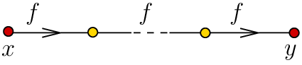

We now put:
| (11) |
where, go over all the trees as above and we only count elements in when the associated virtual dimension is (we will use the same convention in the other examples below). The relation is obtained by using the same type of moduli spaces but with virtual dimension equal to . Notice that if has a single maximum, , then, for degree reasons, is a cycle in the pearl complex (the point here is that the differential is defined over ).
We will omit , , , from the notation if they are clear from the context.
b. The quantum product. In this case with the three functions all defined on . The product is defined by:
| (12) |
where the sum is taken over all the -colored trees with marked points of symbol with , and which are -admissible with and as follows. First, the marking selector verifies: if is of valence at most then ; if is of valence at most , ; if is of valence , and is the -th entering edge (in the planar order) at the vertex (clearly, ), then . In other words, at a vertex of valence , the marked (or incidence) points are the roots of order three of the unity. Finally, the exit rule is , . The virtual dimension in this case is . Schematically, the trees used here and the associated configurations are depicted in Figure 1.
Similar moduli spaces but of virtual dimension are used to show that the linear map defined by (12) defines a chain morphism and thus descends to homology.
A useful remark here is that we can also use instead of the three functions , , only two function and with the same exit rule as above except that for the vertex of valence we require . It is easy to see that this definition provides a product
| (13) |
which coincides in homology with the product given before (see also the invariance properties described at point e). This is particularly useful in verifying the associativity of the product as described at point f below as it allows one to work in that verification with only three Morse functions. Another reason why this description of the product is useful is that, assuming that has a single maximum , we see that if a moduli space used to define (13) is of symbol and of dimension , then and consists of the unique Morse trajectory of joining to . Thus hence is a unity at the chain level for the product defined in (13).
c. The module structure. We now have with one Morse function and one Morse function . We let be the Morse complex of tensored with the ring (endowed with the Morse differential ). The module action is defined by:
| (14) |
where the sum is taken over all the -colored trees of symbol with and which are -admissible for and defined as follows: for all edges of type , , ; if is an edge of type (there can in fact be at most one such edge), then ; , . The virtual dimension in this case is .


The same type of moduli spaces but of virtual dimension serve to prove that this operation passes to homology. However, at this step a modification is needed and has to do with the proof of transversality: we need that in these moduli spaces if a vertex is of valence three, then the corresponding curve is not pseudo-holomorphic but rather it carries a small Hamiltonian perturbation of type:
| (15) |
with well chosen Hamiltonians and and the respective Hamiltonian vector fields (see [MS] and [BC7] for details). The reason why these perturbations are needed will be explained in the next section and we refer to [BC7] for the full construction.
d. The inclusion . In this case we use one Morse function and another Morse function and . The relevant -colored trees with marked points have symbol with , . The marking is chosen as follows: for all the edges of type , , ; for the edge of type , (it is easy to see that the stability condition iv in §3.1 together with the form of the symbol imply that there can only be a unique edge of type . The exit rule is , (notice that, this is the first place where the symbol in the definition of the exit rule at point v in §3.1 is of use; moreover, because the symbol is , the only disk type vertex with the exit edge of type is the one just before the end of the tree). The virtual dimension is in this case and the quantum inclusion is defined by
e. Invariance. Assume given two sets of data and so that the pearl complexes and are defined. We now need to construct a chain morphism:
which induces a canonical isomorphism in homology (we omit the ring from the notation). This morphism is associated to: , a smooth one parametric family of almost complex structures with , , a Morse homotopy (see [BC7] as well as [CR]) between and , a metric on with and . In other words, we use here a slight modification of our standard construction by taking and using trees as at point a, but with replacing , replacing and instead of . The symbol is with and . In particular, both the marked point selector and the exit rule are the same as at point a. The points a,b, c, in §3.1 B. are also modified as follows.
The set is now a subset of the product
where
The flow is replaced by the negative gradient flow, , of with respect to (which is a flow on ) and points a,b, c now apply without further modifications. In short, the curves which appear at the start (and respectively the end) of the edge are -holomorphic where is determined by the second coordinate of the starting point (respectively, end) of the flow line of which corresponds to . Notice that in our construction all intervening curves are genuinely -holomorphic for some in contrast to the continuation method familiar in Floer theory.
The virtual dimension is . The morphism is defined by:
An additional parameter is required to show that the morphism induced in homology is canonical - by constructing a chain homotopy between any two morphisms as above which is associated to a Morse homotopy of Morse homotopies. Perfectly similar constructions provide chain homotopies which proves the invariance of the quantum product and of the module structure.
f. The associativity type relations. The purpose here is to define the moduli spaces needed to prove the associativity of the quantum product as well as the other relations at point ii of Theorem A.
For the associativity of the quantum product we will use three functions , and the moduli spaces to be considered are modeled on trees of symbol with and ; the exit rule is . We will now define a particular family of marked point selectors consisting of one marked point selector for each . This is as in the definition of the quantum product for all vertices of valence and and in case one vertex is of valence then the first two edges arriving at (in the planar order) and the exit edge are attached at the roots of the unity of order - in the same way as for the vertices of valence . The third arriving edge verifies . The moduli spaces used to prove the associativity of the quantum product are
The resulting virtual dimension of this moduli space is (the comes from the additional parameter ).
Both and -dimensional such moduli spaces are needed to verify associativity: the dimensional moduli spaces are used to define a chain homotopy and the dimensional moduli spaces are used to prove the relation . More details appear in [BC7].
To prove the relation with and we use two functions and . The moduli spaces in question are modeled on trees of symbol with , , . The exit rule is . Again we will need to define a special family of marked point selectors, denoted in this case by for . The marked point selector is as at point c for all vertices of valence or . If a vertex is of valence 4 then the marked points are the same as at point c for the edges of type . At this vertex there are also two entering edges of type and the respective marked points are as follows: for the edge colored with , we put ; for the edge , colored with , we put . Finally the moduli spaces needed here are:
We will again need moduli spaces of this sort and of dimensions and . As at point c, to achieve transversality, some of the disks appearing in these moduli spaces will need to be perturbed by using perturbations as described by equation (15). More precisely, in the moduli spaces of dimension , if a vertex is of valence , then its corresponding curve is a perturbed -disk. In the moduli spaces of dimension , the disks of valence as well as the disk of valence (if present) need to be perturbed. Again, for more details see [BC7].
g. Comparison with Floer homology. The version of Floer homology that we need is defined in the presence of a generic Hamiltonian . Consider the path space and inside it the set of (contractible) orbits, or chords, of the Hamiltonian flow . Assuming to be generic we have that is a finite set. Fix a generic almost complex structure .
There is a natural epimorphism and we take be the regular, abelian cover associated to so that acts as the group of deck transformations for this covering. Consider all the lifts of the orbits and let be the set of these lifts. Fix a base point in and define the degree of each element by with being here the Viterbo-Maslov index. Let be a commutative -algebra (e.g. , or or itself but not or ).
The Floer complex is the -module:
The differential is given by where is the moduli space of solutions of Floer’s equation which verify and they lift in to paths relating and . Moreover, the sum is subject to the condition .
The comparison map from the pearl complex
is defined by the PSS method (see [PSS] and, in the Lagrangian case, [BC1], [CL1],[Alb1]) as well as the map in the opposite direction
In our language, the map is defined by counting elements in moduli spaces modeled on trees of symbol with , - thus notice a first modification of the “pearl” construction, the exit of the tree is labeled in this case by an orbit. There will be just one Morse function and the exit rule as well as the marked point selector are as at point a (in §3.2). However, the last vertex in the tree, the exit, will no longer correspond to a critical point but rather to a solution of the equation
| (16) |
so that is an appropriate increasing smooth function supported in the interval and which is constant equal to on . This solution has also to verify , , and so that condition c in §3.1 B which describes the geometric relation associated to the exit edge , is replaced by: “ so that ”. The map is given by using similar moduli spaces but with the first vertex being a perturbed one (the perturbation will use the function ) and starting from an element of . Proving that these maps are chain morphisms and that their compositions induce inverse maps in homology depends, in the first instance, on using one-dimensional moduli spaces as above and, in the second, on yet some other moduli spaces which will produce the needed chain homotopies. For these moduli spaces are again modeled on trees with a single entry and exit, as in the differential of the pearl complex, but both the exit and entry vertices are of the perturbed type as in (16) (with a perturbation for the entry and for the exit). In the case of one of the internal vertices satisfies a perturbed equation but a function with support in an interval of type is used instead of (see again [Alb1],[BC7] for details).
h. The augmentation. Fix a pearl complex where is a algebra (as in §2.1.2). Define
by for all critical points and for those critical points with . Notice that a (local) minimum can not appear in the differential of any critical point y except for and . Indeed, a moduli space modeled on a tree of symbol as at the point a in this section is of dimension and thus can only be of dimension if . Since for each critical point of index there are precisely two flow lines emanating from it, we deduce that and so is a chain map. The same type of argument, now applied to the comparison map constructed in the invariance argument at point e shows that, in homology, commutes with the canonical isomorphisms.
3.3. Transversality
As mentioned before we will not give here the full proof of transversality (we refer to [BC7] for that). However, we will review the main ideas.
Given an -colored tree with marked points as defined in §3.1 we discuss the proof of the fact that, for generic , the associated moduli space is a manifold of dimension equal to the virtual dimension . The finite family of Morse functions defined on or on is fixed throughout the section and it contains at most three functions defined on and two defined on . The only moduli spaces to be treated are those appearing in §3.2.
In the argument, slightly more general such moduli spaces will also be needed. As before, the numbers of entries will always be at most and there will be a single exit. However, we will not impose any particular restriction on the exit rule (in particular, all possible exit rules will be allowed in the inductive argument below). Secondly, we will need to prove the regularity of moduli spaces of type
where is a family of marked point selectors so that at most two of the marked points provided by (and which are associated to vertices of valence at least ) are allowed to take the values in the set . Here where both are connected submanifolds without boundary of dimension at most . These types of moduli spaces have already appeared in the discussion of associativity at the point f in §3.2 and some additional ones will appear in the transversality argument. More precisely, our allowed choices for these sets are as follows. If , then coincides with one of the marked points appearing in the description of the marked point selectors in §3.2 (in other words, is one of the points ); if , then is one of the following two choices or (both have been already used at point f in §3.2); finally, if , then . We will still refer to these moduli spaces by and refer to them as -colored moduli spaces with marked points and, by a slight abuse of notation, will still be referred to as a marked point selector. The virtual dimension of these moduli spaces is given by a formula similar to (10) to which is added another term depending on the dimension of the sets as above and on the valence of the vertices to which these marked points are associated. In view of this, we denote this virtual dimension by .
Let be the moduli spaces associated to -colored trees with marked points which satisfy the additional condition that all the -holomorphic curves corresponding to the internal vertexes have the property that they are simple and that they are absolutely distinct. We recall that a curve is simple if it is injective at almost all points in the sense that and . The curves are absolutely distinct if no single curve has its image included in the union of the images of the others, . By a straightforward adaptation of now standard techniques, as in [MS] Chapter 3 in particular Proposition 3.4.2, we obtain that is a manifold of dimension , in general non-compact, with a boundary consisting of configurations so that some edges in are represented by gradient flow lines of -length (recall that we allow the length of edges to be ). Notice that, in case some perturbed -holomorphic curves appear also in the elements of as at c in §3.2, there is no need to impose any similar condition to them: a choice of generic perturbations insures the needed transversality. To simplify the argument, we focus in the proof below on the case where just a single almost complex structure appears in the definition of our moduli spaces. However, if as for the invariance argument, point e in §3.2, we need to deal with a family of almost complex structures, then the “absolutely distinct” condition only needs to be verified for the disks that are -holomorphic for each at a time and by taking this remark into account the argument below adapts easily to this setting.
The key point is to show that as long as . In turn, the proof of this is by induction. To be more explicit, fix the symbol of the tree . Fix some . The combinatorial data used to define -colored trees with marked points so that is finite. Thus, up to isomorphism, there are only finitely many such trees. Suppose, by induction, that for all -colored trees with marked points of symbol of length at most and with and , we have
| (17) |
To prove identity (17) for it suffices to show that the following simplification step is true:
| (18) |
Indeed, if , the identity (17) together with the regularity of the moduli spaces consisting of simple, absolute distinct curves implies that and the conclusion follows by contradiction.
The key to prove (18) is a structural result concerning -holomorphic disks which is the disk counterpart of the multiply-covered almost everywhere injective dichotomy valid in the case of -holomorphic spheres. One such result is due to Lazzarini [Laz2][Laz1] (an alternative one is due to Kwon-Oh [KO]). Here are more details on this point.
Let be a non-constant -holomorphic disk. Put . Define a relation on pairs of points in the following way:
Denote by the closure of in . Note that is reflexive and symmetric but it may fail to be transitive (see [Laz1] for more details on this). Define the non-injectivity graph of to be:
It is proved in [Laz1, Laz2] that is indeed a graph and its complement has finitely many connected components. We use the following theorem due to Lazzarini (See Proposition 4.1 in [Laz1] as well as [Laz2]).
Theorem 3.3.1 (Decomposition of disks, [Laz1, Laz2]).
Let be a non-constant -holomorphic disk. Then for every connected component there exists a surjective map , holomorphic on and continuous on , and a simple -holomorphic disk such that . The map has a well defined degree and we have in :
where the sum is taken over all connected components .
Two Lemmas, 3.3.2 and 3.3.3, to be stated a bit later, are easy consequences of the theorem above and, as we will see, they reduce our problem to a sequence of combinatorial verifications.
Returning to the proof of (18) we proceed in two steps. First we discuss the argument insuring that all -curves involved are simple. The second step will show that they can also be assumed to be absolutely distinct. We focus here on the case and will comment on the case at the end.
Thus, suppose that is so that and for some internal vertex the corresponding -holomorphic curve is not simple.
In the trees used in this paper a sphere-type vertex does not carry more than three incidence points. Therefore, in case is a -sphere it can clearly be replaced by a simple one and the marked point selector is not modified. This means that we may take in this case to be topologically the same tree as except that the label of the vertex is now instead of . Thus we may now suppose that is a -disk. To deal with this case we will make use of the following consequence of Theorem 3.3.1. We refer to [BC7] for the proof.
Lemma 3.3.2.
Suppose . Then there exists a second category subset such that for every the following holds. For every non-constant, non-simple -holomorphic disk there exists a -holomorphic disk with the following properties:
- (1)
and .
- (2)
is simple.
- (3)
. In particular, if is monotone we also have .
We apply Lemma 3.3.2 to replace the -disk by the simple disk provided by the Lemma. Thus, to prove (18), the relevant tree that we are looking for is identified with except that the vertex will now be labeled by . A slightly delicate point needs to be made concerning the marked point selector corresponding to . The way this is constructed is the following: as , and , the points (where is an incident edge at ) can be lifted to the domain of and used as marked points there. Of course, this works only if all these points, , are distinct. If this is not the case some additional vertices need to be included in the tree so that they correspond to constant disks or spheres which are related to the vertex by edges colored by functions in and of -length.
We still need to verify that . Given that and so this inequality is automatic if because in this case . This is the case if carries two or three marked points all on . The same is true also if carries two marked points, one on the boundary and one in the interior of . Suppose now that carries two boundary marked points, and , and the interior marked point (as at point c in §3.2). In this case the marked point selector for can not be assumed to be the same as that for : the internal marked point for can not be assumed anymore to be as assigned by but can be anywhere inside - in other words in this case . In this situation we have and it is easy to see that . Thus, if we still have so that (17) remains true for the moduli spaces needed to define the module structure without the need to use any perturbations. However, to prove the fact that the operation defined there is a chain morphism we need to use moduli spaces as before but which verify . This is precisely why we use perturbed -holomorphic disks in this case: as mentioned before, the proof of the transversality of the relevant evaluation maps requires only the non-perturbed -holomorphic curves to be simple and absolutely distinct. The same issue appears for both the and -dimensional moduli spaces used to prove the associativity of the module action as in the second part of point f in §3.2 and this shows that the perturbations indicated there are necessary. Full details for these arguments are found in [BC7].
We now pass to the second step: showing that the -curves are absolutely distinct. The main tool is the next result which can be deduced too from Theorem 3.3.1.
Lemma 3.3.3.
Suppose . Then there exists a second category subset such that for every the following holds. If are simple -holomorphic disks such that is an infinite set, then:
- i.
either and ; or
- ii.
and .
This implies that if the -curves in are not absolutely distinct, then there exist two vertices and both corresponding to -holomorphic (unperturbed curves) so that and . The aim now is to show that we can “simplify” both and the tree by eliminating (as well as possibly other vertices and edges) and thus produce a new tree of lower Maslov number and with as well as a new element thus arriving at a contradiction.
There are three different cases to consider:
- i.
and are independent, in the sense that they are on different branches of the tree.
- ii.
is above in the tree, in the sense that by following the tree starting from we reach .
- iii.
is above in the tree.
In the first two cases we obtain the new tree by simply taking the branch in the tree above but containing and pasting it in with in the place of . Thus in the tree the vertex has disappeared and has been replaced with . To avoid confusion we denote this vertex in by . The corresponding pearly element will satisfy for every and . A similar construction can be performed in the third case. Here is a more precise description of this operation in each of the cases i-iii.
In case i we first remove from the branch of the tree lying above (and including ). Then we also remove from the path going from to the branch point below which is closest to . Denote the remaining tree by . We define by gluing to identifying with . This new vertex will be now denoted by . We label by the homology class of and we define at using the marked points of both and except of the exit marked point of which becomes irrelevant now and is hence dropped. See figure 4 for an example.

In case ii, if there is a branch point between and we define as follows. We delete from the branch as in case i above. We also delete from the path between and and denote the remaining tree by . We define as in case i by gluing to identifying with , calling the this new vertex . As in case i above, we label by the homology class of and define using the marked points of both and , excluding the exit marked point of . See figure 5 for an example.

To conclude case ii we need to describe in case there is no branch point between and . In that case, we just define by removing the path between and and identifying with . This new vertex is labeled by the label of and the marked points now are inherited from and except of the exiting marked point of and the corresponding entering marked point of which are now dropped.
Suppose we are now in case iii, i.e. is lower than in the tree. This case is dealt with similarly to ii. In this case, the tree is obtained as before but with the roles of the vertices and reversed: the branch above and containing is grafted to the tree in the place of and the branch leaving from and reaching the first branch point separating and (or the portion in the tree between and if no such branch point exists) is omitted. The new vertex (corresponding to and is now called . Again the -curves associated to the vertices of are the same as the corresponding curves associated to the vertices of except that .
There is yet another point at which care should be taken (in all cases i-iii). It may happen that some of the relevant marked points of and of coincide (again, we disregard those marked points that are dropped as above), and in this case the description given above for is incomplete. If such a coincidence of marked points occurs we need to insert some additional vertices, corresponding to constant -curves, carrying distinguished marked points as well as connecting edges. This modification is straightforward and we will not go into more detail about it.
It now easily follows that the resulting tree has a strictly lower Maslov index than . The dimension verification is also immediate except if carries some internal marked points. If there is a single such marked point and , then we take (because the internal marked point may now take any value inside ) and we still have, as in the reduction to simple disks, . If carries two internal incidence points or if it carries one but , then, by the particular choice of the moduli spaces in §3.2, corresponds to a perturbed -holomorphic disk in contradiction to our starting assumption.
The case is easily reduced to a number of combinatorial problems. The assumptions , and imply that the total number of -curves is relatively small (for example, there are at most two for the verifications involving the pearl complex) so that combinatorial arguments apply in many of these cases. In fact, it is not hard to use directly Theorem 3.3.1 to deal with trees in which the total Maslov index of the vertices represented by -disks is at most (even if there might be additional vertices corresponding to perturbed disks). This covers all the verifications involved with the pearl complex and its invariance, the product and its associativity and invariance, the definition of the module structure and its invariance. This also works for the proof of the relation for . Finally, the remaining case can also be dealt with combinatorially.
3.4. Compactness and the final step
The transversality arguments in the previous section show that our moduli spaces are manifolds. We will start here by describing the structure of the compactification of these moduli spaces. For this, besides the transversality results described before, we only need the Gromov compactness theorem (for disks see Frauenfelder [Fra]). We first remark that given an -colored tree with marked points and an associated moduli space - constructed as described in §3.1- there is a natural Gromov type topology on as well as a natural compactification .
In short, the elements of are modeled on the tree and the only modification with respect to our definition in §3.1 concerns the points a, b, c, at the end of that section. Specifically, the product is replaced by its compactification
where is the Gromov compactification of so that, for each internal vertex , the associated geometric object . The points a,b, and c, are then replaced by the following variants:
- a’.
For each internal edge , the points and are related by a possibly broken flow line (possibly of -length) of .
- b’.
For an entry edge, , let be the critical point labeling the vertex . The point is related to the point by a possibly broken flow line (possibly of -length) of
- c’.
For the exit edge so that the vertex is labeled by the critical point of , the point is related to by a possibly broken flow line (possibly of -length) of .
A remark is needed concerning the marked point selectors. The various marked points which correspond to the same vertex in the configurations described above are again required to be distinct and are given in the same way as that described in §3.2. In particular, each time two (or more) such incidence points “merge” a ghost curve needs to be introduced.
From now on we will only focus on -colored trees that are of virtual dimension and, in view of our transversality results, we may assume that (17) is satisfied so that (the role of the marked point selector is less crucial in this part and we will omit it from the notation). Under this hypothesis, the first key remark is that each element in contains exactly one configuration among the three types below:
- i.
a flow line broken exactly once.
- ii.
a vertex corresponds to a cusp curve with precisely two components (which can be ghosts).
- iii.
a flow line of length .
The reason for this is that if more than a single such configuration occurs we can extract from an object with which is impossible because such a moduli space of negative virtual dimension is regular and thus void.
The second important remark is that the condition insures that no “lateral” bubbling is possible. More explicitly, this means that if the element verifies condition ii, then the incidence points associated to the vertex are distributed among the two components of the cusp curve so that not all of them are in just one component. This happens because, otherwise, the component which does not carry any of these incidence points can be omitted thus giving rise to an object which belongs to a moduli space of virtual dimension lower by at least than which again is not possible.
The last step is to use the description of the compactification given above to verify the various relations required to establish the theorem (as described at the points a, b, c, d, e, f, g, and i in §3.2). The technical ingredient for this verification is gluing. Gluing procedures have already appeared for example in [FOOO] and for full details we refer again to [BC7]. This gluing procedure insures that, when , each element which is modeled on the tree and which verifies exactly one of the properties i, ii, iii above actually belongs to and appears as a boundary element of .
Finally, the verification of the relations mentioned involves in an essential way the fact that our algebraic operations are defined by using -admissible trees. The role of the exit rule (as described at point v in §3.1) is as follows: for a tree with , if verifies ii above, then, due to the fact that “lateral” bubbling is not possible, is also an element of where is the tree obtained from by replacing the vertex by two vertices (corresponding to the two components of the cusp curve associated to ) related by an edge of length whose type is uniquely determined by the exit rule. Moreover, by gluing, each verifying iii is an element in the boundary of a moduli space modeled on a tree obtained from by replacing the two vertices related by the edge of -length by a single vertex. Denote by the parts of the boundary of formed by the points verifying i. and fix the symbol of . When summing over all trees (of virtual dimension ) and of fixed symbol we see that the configurations of types ii and iii cancel (as we will see below, due to the presence of perturbations in some of our moduli spaces, an additional argument is sometimes needed at this point) and so we deduce:
The relations that need to be justified are then obtained by identifying each element of type i with precisely one element of the product where and are the two trees obtained as follows: first, introduce in an additional vertex on the edge which corresponds to the broken flow line and then let , be the two (sub)-trees which have in common only the vertex and whose union gives .
Clearly, in what concerns the comparison with Floer homology - point g in §3.2 - the argument above needs to be modified slightly. The required modification is however obvious and we will not discuss it further. However, a more substantial addition to the argument is needed in the case of the perturbations of type (15) which were introduced in the moduli spaces needed to verify that the module action is a chain map and to check some of the related associativity - as at points c and f in §3.2. This happens in precisely two cases. The first - concerning the fact that the module operation is a chain map - has to do with the identification of an element with an element of the product . The problem here is that, by the definition of the relevant -dimensional spaces at the end of c in §3.2 we see that such a can be viewed as as product of two configurations modeled on two trees and but one of these configurations contains a vertex of valence three which corresponds to a perturbed curve. At the same time both and are moduli spaces of virtual dimension and so, following the definition of the module action and the pearl differential, they do not contain perturbed curves.
The second case concerns the verification of the associativity type relations involving the module action and it arises if the initial curve leading by bubbling to an element is in fact a perturbed curve (verifying (15)), and carrying marked points, two of which are interior points and each of the two components of the resulting cusp curve carries one interior point. The problem in this case is that just one of the resulting cusp curves verifies the perturbed equation and the other one is a usual -holomorphic curve (the definition of the marked point selector in this case implies that the lower component in the tree is the perturbed one) and this configuration does not actually appear as an object of type iii. The reason is that in the relevant moduli spaces all the vertices of valence three correspond to perturbed curves and thus, the configurations of type iii in this case contain a cusp curve with both components being perturbed.
The solution to these two issues turns out to be simple: a further analysis of the moduli spaces involved in both cases shows that if the relevant perturbations are small enough - which can be obviously assumed - then the two types of configurations which are compared in each case are in bijection. This is proved by a cobordism argument which is possible because both the perturbed and the un-perturbed configurations are regular - see again [BC7] for more details.
4. Additional tools
In this section we introduce a number of additional tools which will be useful for the proof of the main theorems and in related computations.
4.1. Minimal pearls
As before, we assume here that is monotone. Suppose that for some almost complex structure and Morse function the pearl complex is defined. It is clear that if is a perfect Morse function, in the sense that the differential of its Morse complex is trivial, then the pearl complex is most efficient for computations. Clearly, not all manifolds admit perfect Morse functions. However, we will see that, algebraically, we can always reduce the pearl complex to such a minimal form (a similar construction in the cluster set-up has been sketched in [CL1]).
It is crucial to work here over a “positive” coefficient ring. We will use in this section . In the algebraic considerations below the fact hat plays an important role.
Let be a finite dimensional graded -vector space and let be a chain complex with a differential which is -linear - in other words is a -chain complex. For an element let with . In other words is obtained from by treating as a polynomial variable and putting . Clearly , . Similarly, for a chain morphism we denote by the -chain morphism obtained by making . Let be the homology of the complex . We refer to this homology as -homology in contrast to -homology which is denoted by .
Proposition 4.1.1.
With the notation above there exists a chain complex
and chain maps , so that: , and induce isomorphisms in -homology and and induce isomorphisms in -homology. Moreover, the properties above characterize up to (a generally non-canonical) isomorphism.
Concerning the the uniqueness part of the statement see also §4.1.1.
Here is an important consequence of Proposition 4.1.1:
Corollary 4.1.2.
There exists a complex , with and so that, for any such that is defined, there are chain morphisms and which both induce isomorphisms in quantum homology as well as in Morse homology and verify . The complex with these properties is unique up to (a generally non-canonical) isomorphism.
We call the complex provided by this corollary the minimal pearl complex and the maps , the structure maps associated to (or shorter, to ). This terminology originates in rational homotopy where a somewhat similar notion is central. There is a slight abuse in this notation as, while any two complexes as provided by the corollary are isomorphic this isomorphism is not canonical. Obviously, in case a perfect Morse function exists on any pearl complex associated to such a function is already minimal. As mentioned before, in the arguments below it is essential that the differential and morphisms are defined over (but the same constructions also work over ; see §2.1.2 for the various Novikov rings available). In case we need to work over we define .
Remark 4.1.3.
a. An important consequence of the existence of the chain morphisms and is that all the algebraic structures described before (product, module structure etc.) can be transported and computed on the minimal complex. For example, the product is the composition:
| (19) |
where are the structural maps given by Corollary 4.1.2 and which correspond to the complexes associated to . There is a cycle in equal to where is the maximum of any Morse function so that is defined and so that has a single maximum; are the associated structural maps. By degree reasons in dimension and and so this cycle is independent on the choice of and of that of the associated structural maps and it coincides with where is the fundamental class of . By a slight abuse of notation we will continue to denote by both the cycle as well as its quantum homology class. In homology, the product defined by (19) has as unity the fundamental class . Moreover, with the simplified description of the quantum product given in (13) - where we obtain a product so that is the unity at the chain level. It also follows from the fact that induce isomorphisms in Morse homology that the “minimal” product described above is a deformation of the intersection product.
b. A consequence of point a is that iff there is some so that . Indeed, suppose that . Then, as for degree reasons is a cycle in , we obtain that it has to be also a boundary. This means that there exists so that . Multiplying by a large enough positive power of gives an element which now lies in and such that . Conversely, if then is a boundary in . On the other hand the cycle represents the unity for the product on just mentioned at point a above. Thus the unity is , hence .
c. It is also useful to note that there is an isomorphism iff the differential in is identically zero.
We now proceed to the proof of the Proposition and of its Corollary.
Proof of Proposition 4.1.1. We start with a useful algebraic property.
Lemma 4.1.4.
Let and be two -chain complexes. If a chain morphism which is -linear is so that induces an isomorphism in -homology, then induces an isomorphism in -homology.
Proof.
Recall that the filtration induces a filtration, called the degree filtration, on any free - module. The resulting spectral sequence induced on any -chain complex is called the degree spectral sequence. Clearly, respects the degree filtration and thus it induces a morphism relating the degree spectral sequences of and . We notice that is identified with the morphism induced by in -homology. Therefore, this is an isomorphism. As we work over this implies that is an isomorphism. ∎
Remark 4.1.5.
a. Under the assumptions in Lemma 4.1.4, the same spectral sequence argument also shows that the chain morphism
induces an isomorphism in homology.
b. Let , be finite dimensional, graded -vector spaces. We claim that a -linear morphism
is an isomorphism if and only if is an isomorphism. Indeed, any such can be viewed as a morphism of chain complexes by assuming that the differentials in the domain and target are trivial. We deduce from Lemma 4.1.4 that, if is an isomorphism, then is an isomorphism. Conversely, if is an isomorphism, then is an isomorphism. As is identified with the quotient morphism
induced by , it follows that is an isomorphism.
We now return to the proof of Proposition 4.1.1. Start by choosing a basis for the complex as follows: so that , , , . For further use, we denote , , .
Clearly, and we will identify further these two vector spaces and denote where are of the same degree as the ’s (the differential on remains to be defined). We will construct and and so that , and . If and verify these properties, then, they induce an isomorphism in -homology and, by Remark 4.1.4, and induce isomorphisms in -homology.
The construction is by induction. We fix the following notation: . Similarly, we put . Notice that there are some generators in which are of degree , namely the ’s of that degree. With this notation we also see that is a sub-chain complex of (because and so , the same type of relation holds for and for we have ) . Assume that is the maximal degree of the generators in . For the generators of we let be equal to , we put on and we also let on . To see that is a chain morphism with these definitions it suffices to remark that if , , then and so .
We now assume defined on , so that are chain morphisms, they induce isomorphisms in homology and . We intend to extend these maps to , . We first define on the generators , which are of degree : , . We let ( when needed, we use the superscript to indicate the maps previously constructed by induction). Here it is important to note that, as , we have that . We consider now the generators which are of degree and we put . This makes sense because . We write and we first see so that, to make sure that is a chain morphism with these definitions, it remains to check that for all of degree . But and as is a chain morphism, we have which implies our identity because . Clearly, induces an isomorphism in -homology and hence in -homology too.
To conclude our induction step it remains to construct the map on the generators of degree . We now consider the difference and we want to show that there exists so that and . Assuming the existence of this we will put and we see that is a chain map and . To see that such a exists remark that and (because is a chain map). Moreover, because . Therefore is a cycle belonging to . But is a chain morphism which induces an isomorphism in homology and which is surjective. Therefore . Thus there exists so that and this concludes the induction step.
This construction concludes the first part of the statement and to finish the proof of the proposition we only need to prove the uniqueness result. For this, suppose and are chain morphisms so that with , and some graded, -vector space and , , , induce isomorphisms in the respective homologies. We want to show that there exists a chain map so that is an isomorphism. To this end we define , . Now and , , are all isomorphisms (in -homology). So is an isomorphism but as we deduce that is an isomorphism. By Remark 4.1.5 b, the map is an isomorphism. ∎
Proof of Corollary 4.1.2. Fix a triple and assume that is defined. Apply Proposition 4.1.1 to this complex. Denote by the resulting minimal complex and the chain morphisms as in the statement of 4.1.1. The only part of the statement which remains to be proved is that given a different set of data so that is defined, there are appropriate morphisms as in the statement. There are comparison morphisms: as well as so that, by construction, both and are inverse in homology and both induce isomorphisms in Morse homology (and these two isomorphisms are also inverse). Define , by and . It is clear that , , and induce isomorphisms in homology. Moreover, as and are inverse in homology and in it follows that . This means by Lemma 4.1.4 that is a chain isomorphism so that is the identity. We now put and this verifies all the needed properties. The uniqueness of now follows from the uniqueness part in Proposition 4.1.1. ∎
4.1.1. Further remarks on minimal models
While the minimal complex associated to -complex is unique (upto isomorphism), this is not the case for the structural maps and . For these maps we expect uniqueness in a weaker sense such as uniqueness upto chain homotopy, however we will not pursue this direction here. On the other hand, we will use minimal models in §5 quite frequently. In fact, in §5 we will have to use the specific choice of the morphisms , (as well as , ) that is constructed in the proof of Proposition 4.1.1. It seems plausible that this can be avoided by axiomatizing more the theory of minimal models, but we will not do this here since we view the minimal model as a purely computational tool.
4.2. Geometric criterion for the vanishing of
Let be a monotone Lagrangian submanifold. Remark 4.1.3 b provides a criterion for the vanishing of . We provide here a more geometric such criterion which is useful when which we will assume in this section.
Denote by the boundary homomorphism and by the composition of with the reduction mod , . Given and consider the evaluation map
where is the group of biholomorphisms of the disk.
For every let be the set of all classes with for which there exist -holomorphic disks with boundary on in the class :
Define:
Standard arguments show that:
- (1)
is a finite set for every .
- (2)
There exists a second category subset such that for every , . In other words, for generic , is independent of .
- (3)
For every and every the space is compact and all disks are simple.
- (4)
For and , the space is a compact smooth manifold without boundary. Its dimension is . In particular, for generic , the number of -holomorphic disks with is finite.
- (5)
For every and the manifolds and are cobordant via a compact cobordism. Moreover, the evaluation maps , extend to this cobordism, hence . In other words depends only on .
- (6)
In fact, the set above can be taken to be the set of all which are regular for all classes in the sense that the linearization of the operator is surjective at every .
Let and let be a generic point. Define a one dimensional -cycle to be the sum of the boundaries of all -holomorphic disks with whose boundaries pass through . Of course, if a disk meets along its boundary several times we take its boundary in the sum with appropriate multiplicity. Thus the precise definition is:
| (20) |
By the preceding discussion the homology class is independent of and . In fact
| (21) |
Proposition 4.2.1.
Let be a monotone Lagrangian submanifold with . If then .
Proof.
Choose a generic . Let be a generic Morse function with precisely one local maximum at a point and fix a generic Riemannian metric on . Denote by , the Morse and pearl complexes associated to , and the chosen Riemannian metric. As discussed in §3.2 b, is a cycle in the pearl complex of and its quantum homology class is the unity.
For degree reasons the restriction of to is given by , where counts pearly trajectories with holomorphic disks of Maslov index . Since is a maximum of , no trajectories can enter (i.e. ). Therefore for every we have
| (22) |
Assume now that . By Poincaré duality there exists an -dimensional cycle in such that
Let be a -cycle representing . Then
for some non-zero scalar . (Of course, is the same as here, since we work over . However we wrote to emphasize that the argument works over every field.) It follows that . But, as is the unity of , we deduce . ∎
4.3. Action of the symplectomorphism group
We now describe a property of our machinery which is very useful in computations when symmetry is present. In this section is any of the rings described in §2.1.2.
Proposition 4.3.1.
Let be a diffeomorphism which is the restriction to of an ambient symplectic diffeomorphism of . Let be so that the pearl complex is defined. There exists a chain map:
which respects the degree filtration, induces an isomorphism in homology, and so that the morphism induced by at the level of the degree spectral sequence coincides with (where is the isomorphism induced by on singular homology). The map induces a representation:
where are the ring automorphisms of preserving the augmentation and are the symplectomorphisms of which keep invariant. The restriction of to takes values in the automorphisms of as an algebra over (here is the component of the identity in ).
Proof.
To ease notation, we omit the ring in the writing of the pearl complexes below.
Assume that is a diffeomorphism which is the restriction to of the symplectomorphism and are such that the chain complex is defined. Let . There exists a basis preserving isomorphism
induced by for all where are obtained by the push-forward of by means of and the symplectomorphism . The isomorphism acts in fact as an identification of the two complexes.
Next, there is also the standard comparison chain morphism, canonical up to chain homotopy
We now consider the composition . It is clear that this map induces an isomorphism in homology and that it preserves the the ring structure and the augmentation (as each of its factors does so). We now inspect the Morse theoretic analogue of these morphisms - in the sense that we consider instead of the complexes the respective Morse complexes . It is easy to see that the Morse theoretic version of induces in Morse homology precisely . But this means that at the stage of the degree filtration the morphism induced by has the form .
We now denote and we need to verify that for any two elements we have . It is easy to see that this is implied by the commutativity of the following diagram:
for any two Morse function and so that the respective complexes are defined. To verify this commutativity, first we use some homotopy , joining to , to provide the comparison morphism and we then use the homotopy to define .
Finally, recall that the module structure of over is defined by using an additional Morse function . If we put we see easily that the external operations defined by using and are identified one to the other via the application (extended in the obvious way to the critical points of ). There is a usual comparison map relating the Morse complex of to that of . Together with the map identifies - in homology - the external product associated to and the external product associated to . At the level of the quantum homology of the composition induces . Therefore, if , it follows that this last map is the identity and proves the claim. ∎
Remark 4.3.2.
It results from the proof above that for to be an algebra automorphism it is sufficient that induce the identity at the level of the singular homology of , e.g. when is homotopic to the identity.
4.4. Duality
We start by fixing some algebraic notation and conventions. Let be a commutative algebra. Suppose that is a free -chain complex. Thus with some graded -vector space. We let
graded so that the degree of a morphism is if takes to for all .
Let be graded such that if is a basis element of , then its dual has degree . There is an obvious degree preserving isomorphism defined by where is a basis of and is the dual basis. We define the differential of , , as the adjoint of :
Clearly, continues to be a chain complex (and not a co-chain complex).
An additional algebraic notion will be useful: the co-chain complex associated to . To define it, for a graded -vector space let be the graded vector space obtained by reversing the degree of the elements in : if , then its degree is . Clearly, .
For the complex as above we let . The complex is obviously a co-chain complex and its differential is a -module map. The cohomology of is then defined as . Obviously, there is a canonical isomorphism: .
A particular case of interest here is when . In this case we denote:
Notice that the chain morphisms of degree are in correspondence with the chain morphisms of degree :
via the formula . Here the ring on the right hand-side is considered as a chain complex with trivial differential.
For and any chain complex as before we let be its -fold suspension. This is a chain complex which coincides with but its graded so that the degree of in is the degree of in . A particular useful case where both duality and suspension appear is in the following sequence of obvious isomorphisms: .
Proposition 4.4.1.
Let . There exists a degree preserving morphism of chain complexes:
which is a morphism of -modules and induces an isomorphism in homology. In particular, we have an isomorphism: . The corresponding (degree ) bilinear map
coincides with the product described at point ii of Theorem A composed with the augmentation . When the pairing is non-degenerate. Moreover, for any the induced pairing:
is non-degenerate.
Proof of Proposition 4.4.1. For any two pearl complexes and the construction at point §3.2 e. provides a comparison chain morphism relating them. There is an alternative way to construct a comparison map
in case and are in general position. In homology, this induces the same morphism as the one provided by the map constructed at point e in §3.2. This alternative comparison map is useful in the understanding of duality. The definition of this map is:
where the sum is taken over all the trees of symbol , , and . We put in this case and . The exit rule - point v in §3.1 B - needs to be slightly modified for these trees: in the tree there is one special vertex so that for all vertices above it the exit rule is , for all the vertices below it the exit rule is and at the exit rule is . Condition iv in §3.1 B is also slightly modified in the sense that the vertex is allowed to verify . The marked point selector is as at point §3.2 a. The duality map
is defined as the composition of two maps, the first is the canonical identification of chain complexes obtained by “reversing” the flow (which sends each critical point to ) and the second is where is a Morse homotopy between and so that . To prove the identity , let be another Morse function in generic position with . In homology where is a Morse homotopy from to and is a Morse homotopy from to . Thus we also have . The relation we want to justify follows by comparing the moduli spaces associated to the trees of symbol with , used in the definition of and the moduli spaces associated to trees of symbol (with , ) where , , used in the definition of the product at the point b in §3.2. Here is the unique minimum of the function . Indeed it is immediate to see that the -dimensional such moduli spaces are in bijection and this implies the claimed identity.
It remains to prove that the pairing (and thus ) is non-degenerate when . From now on we put and omit it from the notation.
Let be a finite rank free -chain complex (e.g. ). Consider the following pairing:
| (23) |
which is defined as follows. Given two classes , choose cycles representing them, , , and define . It is easy to see that is well defined. We will prove below the following.
Lemma 4.4.2.
The pairing is non-degenerate.
Note that in view of the canonical isomorphisms the non-degeneracy of (for ) implies that is non-degenerate.
We now proceed to prove Lemma 4.4.2. Given denote by the space of -linear morphisms that have degree . Consider now the following canonical map:
defined as follows. Given , choose a cycle that represents . Clearly, descends to a map which we define to be . It is easy to see that the map is well defined. Note also that we have
Lemma 4.4.3.
Let be as above. Then for every the map is an isomorphism.
Before proving this lemma that let us see how it implies the non-degeneracy of (hence that of ).
Proof that is non-degenerate.
Let . Choose a homomorphism with . Extend to a an -linear homomorphism (this extension can be done by linearity over in degrees and by in all other degrees). Clearly .
Assume now that . Then is a non-trivial homomorphism. This means that there exists and such that . As it follows that . Put . Clearly , which implies that . This concludes the proof of the non-degeneracy of , modulo the proof of Lemma 4.4.3. ∎
To prove Lemma 4.4.3 we need some more preparation. Let be a commutative graded ring and a graded -module. Denote by the projection on the ’th component of . Let be a submodule. We say that is a graded submodule if for every we have for every . In that case the grading of induces a grading on and becomes a graded -module by itself. Note that not every submodule of a graded module is graded. However:
Lemma 4.4.4.
- i.
A submodule is a graded submodule iff it is generated (over ) by a collection of homogeneous elements. In particular, if are graded submodules then so is .
- ii.
Let . Let be a free finite rank graded -module and a graded submodule. Then there exists a graded submodule which is a complement of , i.e. .
Proof.
The proof of statement i is straightforward, so we omit it.
We prove ii. Choose a homogeneous element (if there are no such elements clearly ). Put . We claim that . Indeed, assume that for some . As is homogeneous and is a graded submodule, all the homogeneous components of must lie in . In particular there exists such that . As is invertible it follows that . A contradiction.
We now continue the same construction inductively, namely we choose a homogeneous element . We claim that . The argument is similar to the preceding one (for ). The point is that is a graded submodule. Put . Clearly we have . Note also that and are both graded submodules of .
Continuing this inductive construction we obtain, after a finite number of steps , the desired complement which satisfies . It is important here that is free of finite rank and that is a PID. These two conditions assure that every submodule of is also free with rank the rank of . In particular the process of defining concludes in a finite number of steps. ∎
Remark 4.4.5.
We remark that the statement at point ii does not seem to hold if we replace by more general graded rings . In order for the proof above to work we need that every non-trivial element in each () is invertible. This obviously holds for , but not for for example.
Coming back to a finite rank free -chain complex , denote by the cycles and by the boundaries. Note that both and are graded -submodules of . The following Lemma is an immediate consequence of Lemma 4.4.4- ii.
Lemma 4.4.6.
There exist graded -submodules and such that and split as direct sums of graded -modules:
In particular, the restriction of to , is an isomorphism and . Moreover, is an acyclic complex and .
This decomposition is of course not canonical.
Proof of Lemma 4.4.3.
We first show that is injective. Suppose that . Choose a cycle representing . As we have and since is a cycle we also have . Define by and . Clearly we have which means that is a boundary, hence . This shows that is injective.
Remark 4.4.7.
a. The relation between the duality above and Poincaré duality is as follows: in case in the statement is replaced with the Morse complex of some Morse function (and we take ) we may define the morphism as a composition of two morphisms with the first being the usual comparison morphism and the second given by . We have the identifications and the morphism described above induces in homology the Poincaré duality map: .
b. Proposition 4.4.1 also shows that together with the bilinear map is a Frobenius algebra, though not necessarily commutative.
c. The quantum inclusion, , the duality map, , and the Lagrangian quantum product determine the module structure by the following formula (which extends (6)):
| (24) |
where , . Of course, here so that it can be evaluated on . As in formula (6), the pairing on the left side is the -linear extension of the standard Kronecker pairing.
4.5. Wide Lagrangians and identifications with singular homology
Let be a monotone wide Lagrangian. This means that there exists an isomorphism . However, in general there is no such canonical isomorphism!
To explain this better, denote by pairs of Morse data. For any two pairs and and any two choices of almost complex structures and denote by the canonical isomorphism between the pearl homologies (as described at point e in §3.2). Denote by the canonical isomorphism between the Morse homologies associated to and . From this point of view, is identified with the family of homologies related by the canonical isomorphisms mentioned above. Similarly, the quantum homology is identified with the family of homologies together with the canonical isomorphisms . Therefore, specifying a map is equivalent to having a family of maps indexed by regular pairs such that the following diagram commutes for every two such pairs , :
| (25) |
Of course, in order to define such a family of maps it is enough to choose a reference pair , define and then all the rest of the are uniquely determined.
The point is that, in general, these choices do not lead to a canonical map . To illustrate this, consider for simplicity the case when admits a perfect Morse function and consider only Morse data where is a perfect Morse function. Write the pearl differential as , where is the Morse differential. As is perfect we have , so that . Moreover, since we assume that is wide, a dimension comparison shows that must vanish too (for otherwise the rank of would be smaller than that of ). Thus for every pair as above. It follows that:
At first glance it seems that a natural isomorphism between the singular and quantum homologies can be defined by for every for every (with the Morse function in being perfect). A more careful inspection shows that if we define the isomorphisms in this way the diagram (25) might not commute. A close look at the definition of the comparison morphism from point e in §3.2 (see also an alternative description in the proof of Proposition 4.4.1) shows that might differ from by some quantum terms. In fact we have:
| (26) |
where the term maps to and is defined by counting elements in some moduli spaces involving and -holomorphic disks with total Maslov index . (See the precise description in the proof of Proposition 4.4.1 in §4.4.) It is not hard to write down examples where some of the quantum terms do not vanish (see [BC6, BC7]). In fact, this turns out to be the case for the Clifford torus (see §6.2).
Despite the above there are situations in which a canonical isomorphism exists, at least in some degrees.
Proposition 4.5.1.
Let be a monotone Lagrangian (not necessarily wide or narrow).
- i.
For every there exists a canonical isomorphism . Moreover, this isomorphism maps the fundamental class to the unity in .
- ii.
If is not narrow then the isomorphism from i exists also for .
- iii.
If is wide, the isomorphism induces a canonical embedding for every . In particular (for wide Lagrangians), if we have a canonical isomorphism .
Proof.
Let be a a pair formed by a Morse function and a Riemannian metric on and let be an almost complex structure on such that the pearl complex as well as the Morse complex are defined. Throughout the proof we will assume without loss of generality that has a unique maximum which we denote by .
Write the pearl differential on as
where is the Morse differential and is an operator acting as . For degree reasons we have:
| (27) |
Moreover, on and on , where .
Point i now easily follows since is a -cycle iff it is a -cycle and is a -boundary iff it is a -boundary. Therefore, the map
descends to an isomorphism in homology. As represents the fundamental class, clearly sends to the unity of . This completes the proof of i except of the canonicity of which will be proved soon.
We turn to point ii. We claim again that is a -cycle iff it is a -cycle and is a -boundary iff it is a -boundary. Indeed, the claim is obvious for boundaries since on . It remains to show that and -cycles coincide on . Let . We have . This implies that if is a -cycle then it is also a -cycle. Suppose now that is a -cycle. We then have . If then which implies that is a boundary hence and is narrow, contrary to our assumption. Thus and is a -cycle.
We can now extend the definition of to by , and as before descends to an isomorphism in homology.
To conclude the proofs of points i, ii it remains to show that is canonical in the sense discussed before the statement of the proposition. To see this, write the map as to denote the relation to the data . For degree reasons it follows that the maps in (26) vanish on for , hence the squares in (25) commute. This completes the proof of the first point of the proposition.
We now turn to the proof of iii. Consider the canonical map induced by the extension of coefficients . The embedding is induced by the map . So, the proof is reduced to showing that is an injection. To see this, let be a -cycle with non-trivial Morse homology class , where . By what we have just proved, is also a -cycle. We have to prove that , when viewed as an element in , is not a -boundary. Consider the minimal model together with the structural map as constructed in §4.1. Recall that by that construction , hence . On the other hand, by 4.1.3 c, the differential of vanishes because is wide. As is a chain map it follows that cannot be a -boundary. ∎
5. Proofs of the main theorems
This section is focused on proving the three main theorems of the introduction.
Before we go on with the proof we would like to make a small but useful algebraic observation which will be used many times in the sequel. Consider the graded vector space endowed with the grading coming from both factors. Let be a homogeneous element (of degree ). Then we can decompose in a unique way as:
Suppose now that for some . In that case we will say that contains . (Note that this can happen only if .) Then, as , , the decomposition of cannot contain terms with of higher order than , i.e.
We will abbreviate this by writing , where stands for terms of lower order in . Similarly, if a homogeneous element contains for some , then must have , where stands for terms of higher order in .
A similar discussion applies to homogeneous elements in the positive quantum homology , as well as in the positive pearl complex in case the function has a unique maximum and a unique minimum.
5.1. Proof of Theorem 1.2.2
The argument is based on the minimal model machinery from §4.1. Consider the pearl complex and recall from §4.1 that there exists a chain complex , unique up to isomorphism, and chain morphisms , so that , (where is obtained from by putting ) and , , , induce isomorphisms in quantum and Morse homologies. By Remark 4.1.3 the quantum product in can be transported by the morphisms and to a product which is a chain map and a quantum deformation of the singular intersection product and so that is the unity at the chain level (notice though that, as the maps and are not canonical, this product is not canonical either). As discussed before we put . As in the statement of the theorem we assume that is generated by . In view of Remark 4.1.3 b. the first point of the theorem reduces to the next lemma.
Lemma 5.1.1.
Suppose that . If , the differential of the minimal pearl complex, does not vanish, then is a boundary in , , and .
Proof.
There are two possibilities: either on , or on that homology.
Assume first that on . We claim that everywhere. To show this we will prove by induction that on for every .
Indeed, for this is true since implies that on , and moreover we have assumed that on . Assume now that the assertion is true for some and let . By the assumptions of Theorem 1.2.2 we can write where each is expressed as (classical) intersection products of elements from . We now claim that for every . To see this write with , where is the classical intersection product. We then have and we write . At the same time
| (28) |
with . (Recall that ). By the induction hypothesis we have , hence . The same argument shows that for every . It follows that . This proves that on and completes the induction.
We now turn to the second case: on . First note that we must have . Indeed, if then by degree reasons on and by what we have just proved we obtain everywhere, a contradiction. Thus . By degree reasons again it follows that sends non-trivially to . Thus there exists such that . This implies that is a boundary. As is the unity of we also obtain . ∎
We now pursue with the proof of the second point of Theorem 1.2.2. Thus we assume that is narrow and so is a boundary in and . Let be the constant in the statement of the theorem, when and when . Notice that the degree component of is one-dimensional. This implies that, despite the fact that the minimal pearl model is determined only up to a non-canonical isomorphism, the generator in degree is canonical. It will be denoted (as before) by .
In the following lemma we denote the differential of the complex by to distinguish it from its extension defined on . The main step is:
Lemma 5.1.2.
Either there exists some so that or there are so that , where in both cases .
Proof.
As is narrow, the first point of Theorem 1.2.2 implies that . Assume first that . Then by definition . In this case, as the proof of Lemma 5.1.1 shows, there exists such that . Thus satisfies the statement of our lemma with .
We will assume from now on that , and so . Let be an element of maximal degree so that contains for some . More precisely, denote by the generator (so that ). We require that is of minimal degree so that . (Here and in what follows we extend the Kronecker pairing to by linearity over .) Note that such a must exist, since is narrow hence must be a -boundary for some .
If , the statement of our lemma is verified with and because . Therefore we assume from now on that . We know that generates as an algebra. In particular, implies that is decomposable with respect to the intersection product. We now write
(Of course, can be a sum of such products but this does not make any difference in the argument and, in terms of notation, it is simpler to assume that just one such monomial appears.) Now
By the maximality of , and the fact that , we see that the second term on the left vanishes and we also get that for either or , say (the other case is similar) we have for some . We now write and we deduce that for some we have . Notice that . We put (clearly and we will show below that ). We now get:
Thus, and the statement of our lemma will be verified with and .
It remains only to check that . Assume by contradiction that , or equivalently that . This implies that . But for degree reasons this cannot happen since . A contradiction. ∎
To prove the second point of Theorem 1.2.2 we will use Lemma 5.1.2 to show that is uniruled of order . For this, we fix a generic almost complex structure as well as a point . Fix a Morse function and a Riemannian metric on so that the pair is Morse-Smale. Moreover, we choose so that is its unique maximum. We also pick a second Morse function so that the pair is also Morse-Smale, and and are in general position. We assume that is generically chosen so that and are both defined as well as the relevant product. As above, we let be the minimal pearl complex and we fix , the structure maps associated to and, respectively, to as constructed in the proof of Proposition 4.1.1 in §4.1.
The following technical result is an easy consequence of the proof of Proposition 4.1.1 and is valid independently of whether is narrow or not.
Lemma 5.1.3.
- i.
If there exists so that , , then there exists so that with .
- ii.
Let be a homogeneous element such that , . Then there exists such that with .
Proof.
We begin with point i. As in the proof of Proposition 4.1.1, change the basis in so that the generators forming the new basis are of three types and so that and are in bijection and (where is the Morse differential). For we denote by the element so that . As we have . The map is defined so that for , ( is the Morse homology class of ), for , and for , . Let be a generator of the highest degree among the the elements of with the property that there exists with (since for , for and with , there must be such a ). Write
We now have:
Note that and therefore by the maximality of none of the terms can contribute an , to that sum. Moreover, none of the terms can contribute to that sum since of an element in is divisible by . It follows that there exists such that the term contributes the element . As it follows that and . As the degree part of is , and , do not contain elements of degree , it follows that . As is a linear combination of pure critical points (it doesn’t involve ’s) we now obtain that (we work here over so ). Finally, there must be a critical point participating in (which is a linear combination of critical points) so that . This completes the proof of point i.
We turn to the proof of ii. Write
| (29) |
with . Note that and that by the construction of and in the proof of Proposition 4.1.1 in §4.1 we also have . Recall also that . Using this, and applying to both sides of (29) we obtain:
Clearly not all of can vanish (where, as before, is the generator). Let be an index such that . We then have . By point i just proved, there exists and such that . ∎
We continue with the proof of point ii of Theorem 1.2.2. We begin by analyzing the first possibility resulting from Lemma 5.1.2: for some with .
Consider the map . As the degree part of consists of only, we have . By the definition of there exists such that . Write . We have: . Thus there exists such that . There are two possibilities: either or . In case we must have hence and it follows that . The element might not be a single critical point of but a linear combination of such. However there must be a critical point participating in the linear combination such that . In case we obtain and as we deduce from 5.1.3 that there exists so that with . Summarizing, we see that in both cases ( and ) that there is so that with . This implies that there exists a non-constant -disk through of Maslov index at most .
It remains to discuss the second case: . The argument is similar. By definition . Write , , with , being homogeneous elements. The equality implies that there exist such that . Write . We get that there exists such that . Now there are two possibilities: either or .
In the first case () we get and so by Lemma 5.1.3-i there exists such that with . It follows that there exists a non-constant -disk through with Maslov index .
In the second case () we have hence and . If there exists a non-constant -disk through with Maslov index . In case we have hence for degree reasons (and , where is the maximum of ). It follows that . We have , for otherwise so which is impossible in view of our starting equality with and . Thus with . By Lemma 5.1.3- ii there exists with with and it follows that there exists a non-constant -disk through with Maslov index . This concludes the proof of Theorem 1.2.2. ∎
5.2. Proof of Theorem 1.2.3
Recall that we now suppose that is point invertible of order . This means that in the quantum homology of with coefficients in there exists , with and so that . Recall that here . Denote . Clearly, we also have in , .
We start with the point i. of the theorem. We first notice that the relation implies and as we have and so . We now use the module structure
to write:
| (30) |
We need to analyze equation (30) at the chain level. For this, we fix a Morse function with a single maximum as well as a Morse function with a single maximum and a single minimum . We also fix Riemannian metrics and on and . The Morse complex of tensored with will be denoted by . We also fix a minimal pearl complex for , , together with the two associated structural maps and as in §4.1. We use the module operation (on the chain level) in the form:
by transporting the module operation via the structural maps , , i.e. for , we define .
We write
| (31) |
Note that there are no classical terms here (i.e. ) for degree reasons, since .
Lemma 5.2.1.
There exists such that .
Proof.
We write as a sum of three terms: with
and . Notice that because , , .
Choose a cycle which represents . We have:
and thus, .
We now claim that . To see this, first note that . Write , with . We have , hence for every . Thus . Assume by contradiction that . Then and so , hence and . This is impossible in view of our assumption that . This proves that .
We now have:
| (32) |
From this equality we deduce and the statement of the Lemma. Indeed, if , then is a boundary in which implies that is narrow, contradicting our assumption. ∎
We continue with the proof of point i of Theorem 1.2.3. In view of Lemma 5.2.1 choose the minimal index such that . We have . ( stands for higher order terms in .) We now have: . But , hence . Note that the classical term in vanishes and so where and . As it follows that . By the definition of the moduli spaces giving the module action (in §3.2), this implies the claim at point i of our theorem: for a generic there exists a non-constant -disk with and such that . In particular
| (33) |
This completes the proof of point i of our theorem.
We now turn to the proof of the point ii of the theorem. Recall that and that . By assumption is wide so , hence by (32) we get . Expending this equality gives:
where we have written (with ). The key remark is that:
| (34) |
This means that . Write , where . It follows that there exists such that . Finally, writing we deduce that there exists such that
Put . There are two main cases to be considered: (i.e. ) and (i.e. ). Before considering each case it is important to note that as we always have .
Case 1: . We have with and we deduce from Lemma 5.1.3 that there exists a critical point such that with . It follows that there exists a non-constant -disk through with Maslov index , which proves the desired uniruling property of . In view of (33) we also have
Case 2: . This means that , hence . Therefore
| (35) |
There are again two cases: and .
Case 2-i: . We obtain from (35) that there exists a non-constant -disk through with Maslov index . As in case 1 above we also have
Case 2-ii: . We will show now that this case is impossible. To see this, first note that by (35) we have that , hence , . This implies that . Write , where are homogeneous elements. Recall that . Therefore
It follows that there exists such that , hence . Clearly this equality takes place in the image of the inclusion defined by , therefore we actually have in :
| (36) |
Note also that by the definition of we have . We will now show that such a relation is impossible in quantum homology. To see this note that since would give which is possible only if which is not the case. As , the relation (36) implies that there exists a homology class with such that . In particular, for generic , the moduli space of (simple) -holomorphic rational curves in the class which pass through a given point in and intersect a cycle representing is not empty. To estimate the dimension of this space denote by the space of simple rational curves in the class and by the group of biholomorphisms of . Consider the evaluation map
The moduli space in question is , where recall that is a Morse cycle representing and stands for the unstable submanifolds associated to the critical points in . By transversality we obtain the following dimension formula:
On the other hand, from (36) we have . Putting this into the dimension formula we get , contradicting the fact that this space is not empty. This rules out Case 2-ii and concludes the proof of Theorem 1.2.3.
∎
5.3. Proof of Theorem 1.2.7
We first recall the definition of the spectral invariants as well as some other basic facts and we fix some conventions.
Consider a generic pair consisting of a -periodic Hamiltonian and an almost complex structure so that the Floer complex is well defined. (Here, is the Floer complex for periodic orbits Floer homology.) Let where is a contractible -periodic orbit of the Hamiltonian flow of , is a disk-capping of (i.e. ) and the equivalence relation is if and . Notice that is a -module (we recall that ), the elements of acting by changing the capping: , where . As is a -module we will define the Floer complex of interest here as: endowed with the usual Floer differential.
Fix also a Morse function as well as a Riemannian metric on so that the pearl complex is well defined.
We need to provide a Floer-theoretic description of our module operation which involves the two complexes above. This is based on moduli spaces similar to the ones used in §3.2 c except that the vertex of valence three in the string of pearls is now replaced by a half-tube with boundary on and with the end on an element . The symbol of the tree is . The total homotopy class of the configuration obtained in this way is computed by using the capping associated to to close the semi-tube to a disk and adding up the homotopy class of this disk to the homotopy classes of the other disks in the string of pearls. More explicitly, a half tube as before is a solution
of Floer’s equation
| (37) |
with the boundary conditions
The marked points on the “exceptional” vertex which corresponds to are so that the point is an exit point for a flow line and is the entry point. Both compactification and bubbling analysis for these moduli spaces are similar to what has been discussed before to which is added the study of transversality and bubbling for the spaces of half-tubes as described by Albers in [Alb2]. As described in [Alb2], an additional assumption is needed for this part: is assumed to be such that no periodic orbit of is completely included in .

Counting elements in these moduli spaces defines an operation:
Fix a Morse-Smale pair on and let be the corresponding Morse complex tensored with . Recall the module action defined in §3.2 c:
There are maps induced by the inclusion :
which we will denote in both cases by .
We will now use the Hamiltonian version of the Piunikin-Salamon-Schwarz homomorphism [PSS]: . Standard arguments show that there is a chain homotopy which verifies:
| (38) |
for every , .
The Floer complex is filtered by the values of the action functional
where , with a contractible -loop in and a cap of this loop. This action is compatible with the action of and we extend it on the generators of by: (where is the monotonicity constant). The filtration of order of the Floer complex, , is the graded -vector space generated by all the elements of action at most .
We emphasize that all the homology and co-homology classes to be considered below are homogeneous. We now recall the definition of spectral invariants following Schwarz [Sch] and Oh [Oh7]. Fix and define the spectral invariant of by:
| (39) |
where is the morphism induced in homology by . Notice that by convention we have . Assuming that is normalized, it is well known that depends only on the class and on , and is therefore denoted by . We refer the reader to [Oh7, Oh5, Oh6, Oh1, Sch, MS] for the foundations of the theory of spectral invariants. See also [Vit] for an earlier approach to the subject.
Let be a monotone Lagrangian submanifold. Theorem 1.2.7 is an immediate consequence of the first part of Lemma 5.3.1 below. To state it we fix some more notation. As discussed before, the inclusion induces a map which is canonical in homology. We continue to denote the induced map in homology by too. Denote by the image of and notice that is a module so that it makes sense to say whether a class is divisible by in : this means that there is some so that .
Lemma 5.3.1.
- i.
Assume that , are so that is not divisible by in and . Then we have the following inequality for every :
- ii.
The second point of the lemma is an extension of a result of Albers [Alb2].
Before proving Lemma 5.3.1, we show how it implies Theorem 1.2.7. Indeed, if is not narrow, then is not trivial and we have which implies the first point of Theorem 1.2.7 because, for degree reasons, is not divisible by in . Moreover, if is point invertible of order , then there is so that . Therefore, setting we get and by applying the lemma for , , we deduce Theorem 1.2.7 ii. ∎
Proof of Lemma 5.3.1.
i. We fix . By inspecting the definition of depth in §1.2.3 we see that the inequality we need to prove is reduced to showing that for every normalized Hamiltonian with there exists a loop such that:
| (40) |
By a small perturbation of we may assume that no closed orbit of is contained in .
Given any , in view of the definition of , we may find in a cycle with . Write where are generators of and , . Represent also as a cycle in , with , . Similarly, represent also by a cycle in . From equation (38) we deduce that , where is the differential in . Write with , (note that here we cannot assume anymore that only). The fact that is not divisible by in implies that there is some with . But this means that there are and so that (where stands for other terms). This means that there are critical points (participating in and ) so that the moduli space (described at the beginning of the section), of symbol and with , is not void. We now consider an element and we focus on the corresponding half-tube (which is part of ). The usual energy estimate for this half-tube gives:
hence:
We now claim that:
| (41) |
Indeed, equals the symplectic area of all the disks in the area of the tube the area of the cap corresponding to . The inequality (41) now follows because the disks in are -holomorphic hence their area is non-negative. But now and as , we obtain:
so that by taking we deduce inequality (40).
ii. Given a Hamiltonian with , a Morse function , a generic metric and a generic almost complex structure we will define a chain map
so that the maps induced in homology by and by are equal. To describe this map, fix a particular capping for each contractible -periodic, orbit of the Hamiltonian vector field of . We denote these pairs by .
For a critical point we define
| (42) |
where the moduli spaces are similar to the ones used in §3.2 d except that the last (exceptional) vertex there as well as its exiting edge are replaced here by a Floer semi-tube; the Maslov index is the sum of the Maslov indices of the disks in the chain of pearls summed with the Maslov index of the tube glued to the disk with reversed orientation. More precisely, the moduli spaces used here correspond to trees of symbol . An element consists of a pair where is a Floer semi-tube
verifying Floer’s equation (37) with the boundary conditions
and is a string of pearls in associated to , starting at the critical point and so that the last incidence condition is
In other words, is an element as of a moduli space as those considered in the construction of the pearl differential §3.2 a except that the end point is not but . The Maslov index is given by where is the disk with the opposed orientation compared to , and indicates the surface obtained by gluing the tube and the capping disk along . The sum in (42) is taken over all such that . It is easy to see that the definition of does not depend on the specific choice of the cappings associated to each .
The regularity issues for the moduli spaces are similar to those discussed before. Finally, standard arguments show that by extending this definition by linearity over we obtain a chain map and that, the map induced in homology by coincides with .
The next step is to establish an action estimate for the configurations considered above. We recall that if is a capped orbit as above, the element is a generator of and its action is . The energy estimate associated to gives:
and so
Clearly, and as we deduce
| (43) |
Let , and let , be a pearl cycle that represents . Write . Consider any of the terms in this sum, say . There exists and a critical point participating in , so that contains . As is -linear this means that contains . From (43) we now obtain
Finally, since and coincide in homology we can represent as a linear combination of of generators of each of action at most which implies our claim. ∎
Remark 5.3.2.
- a.
Sometimes the point ii of Lemma 5.3.1 can be used to estimate from above spectral invariants of homology classes . For example, it is easy to see that , where is the map induced by the inclusion . Therefore whenever we obtain for any .
- b.
In a point invertible manifold the first part of Lemma 5.3.1 provides an estimate from below of and so, in view of the proofs of the intersection results discussed in Corollaries 2.4.1 and 1.2.8, it is particularly important to get also an estimate from the above. The natural idea is to write for some class . However, there are cases when is not in the image of this map - see for example the case of the quadric described in §6.3.3.
- c.
In case we have , where is the set of contractible -periodic orbits of together with all possible cappings (modulo the usual identifications) . In this case the map can be written as where the moduli space contains configurations as those in but with the additional condition that . Indeed, as any element can be written uniquely as some .
If additionally, we have , then a dimension count shows that for the configurations used to define we have and so there are no -disks present in the definition of . Under these assumptions coincides with a map introduced by Albers in [Alb2].
- d.
It is possible to define a pseudo-valuation as follows. Notice first that for any there exists so that . Define
It is easy to see that is well defined, and that it verifies iff , iff , , , and . A similar function to has already been considered by Entov-Polterovich [EP2] in the context of ambient quantum homology. The inequality at point i of Lemma 5.3.1 can now be reformulated as:
5.4. Proof of Theorem 2.4.1
Recall the setting of this theorem. Given , monotone Lagrangian submanifolds we have the two associated rings , be the associated rings, graded by and as well as the ring where , . Recall also the two canonical maps: the quantum inclusion and , defined by . The claim of the theorem is that if the composition:
does not vanish, then and intersect.
We start the proof with a little more preparation. First note that since is a -module we can naturally extend the definition of periodic orbit Floer homology to coefficients in as the homology of the complex . We denote this homology by . Moreover, the PSS isomorphism naturally extends to this case and we get an isomorphism . Similarly, we can extend the action functional to the generators of by defining: . Here , , are the monotonicity constants of the Lagrangians. (Clearly, , unless in which case we anyway have , hence .) It is easy to see that this extension of the action is well defined. With these conventions we have as before a filtration on by action and we can define spectral numbers for every , , in a standard way. A straightforward algebraic argument shows that for classes (as well as , ) these “new” spectral numbers coincide with the usual ones, i.e. . (The point is that is a free module over .) We will also need the ring . As before we have
Next we remark that Lemma 5.3.1 continues to hold if we replace by one of the ’s, say , replace by , by and the condition that “ is not divisible by in ” by “ is not divisible by in the image of the map ” with the canonical “change of coefficients” map . The proof of the lemma carries out to this case without any essential modifications.
Since there exists so that . From the modified version of Lemma 5.3.1 discussed above, we deduce that for some constant depending only on and for any we have
Now assume by contradiction that . Pick a normalized Hamiltonian which is constant equal to on and constant equal to on with . This immediately leads to a contradiction and concludes the proof of Theorem 2.4.1 ∎
We now pass to the proof of Corollary 2.4.3. Put and let be a non-narrow monotone Lagrangian. The claim follows if we show that if is not divisible by in , then . We first fix a Morse function and a metric on as well as an almost complex structure on so that the pearl complex is defined. We assume that has a unique minimum . To simplify the notation, we put .
By the non-degeneracy part in Proposition 4.4.1 there exists a class which is non-zero and is represented by a pearl cycle of the form with . A priori this cycle belongs to , but as and all the the powers of in this cycle must be non-negative. Thus, in fact this cycle is in and . In view of the coefficients extension morphisms we will view from now on as an element of the image of these maps i.e. . Here we have used again the ring and the coefficients extension morphisms induced by the obvious inclusions .
As extends (at the chain level) the inclusion in singular homology we can write with . Notice that because and is a free -module. Taking this into account, we now apply to and we obtain:
| (44) |
where we have denoted and . It is important to notice that in fact . Now suppose by contradiction that . As identity (44) implies that the second term on its right-hand side belongs to . This can only happen if for every with we have , so that . It now follows that is divisible by , and obviously this divisibility property continues to hold also in . A contradiction. ∎
6. Various examples and computations.
The first three subsections below contain the proofs of the computational theorems in §2.3 and of their corollaries from §1.2.5. The last subsection contains the justification of Example 1.2.10.
6.1. Lagrangians in with .
We recall our notation: we denote by the class of a hyperplane so that in the quantum homology we have:
We will use quantum homology with coefficients in and so we recall that , where , , and becomes a -module by . Obviously, is invertible in so that the existence of the module action claimed in Theorem A directly implies the first part of:
Lemma 6.1.1.
Let be a monotone Lagrangian with . Then is -periodic, i.e. for every and the homomorphism given by is an isomorphism for every . Moreover, .
Proof.
The only part that still needs to be justified is that . But if , then and by Theorem 1.2.2 i we deduce that is wide (take in that theorem). The first part of the lemma implies in this case that is -periodic which is impossible by degree reasons. Indeed, but as we have . ∎
Remark 6.1.2.
The first part of Lemma 6.1.1 was proved before by Seidel using the theory of graded Lagrangian submanifolds [Sei2]. The -periodicity in [Sei2] follows from the fact that admits a Hamiltonian circle action which induces a shift by on graded Lagrangian submanifolds. Note that this is compatible with our perspective since that -action gives rise to an invertible element in (the Seidel element [Sei1, MS]) whose degree is exactly minus the shift induced by the -action. In our case the Seidel element turns out to be .
We now focus on our main object of interest in the subsection.
Lemma 6.1.3.
Let be a Lagrangian submanifold in . If then is monotone, , is wide and as a graded vector space we have . Moreover, for every .
Proof.
Since it is easy to see that is monotone. Moreover, a simple computation shows that the minimal Maslov number of is with . We already know from Lemma 6.1.1 that so that is generated as an algebra by . Thus, by Theorem 1.2.2 i, is wide so that, again by Lemma 6.1.1, we deduce that is -periodic. This -periodicity implies (for degree reasons) that cannot be , hence and . Moreover the -periodicity implies that for every . Similarly we have: . Applying the -periodicity again we obtain for every . Summing up we see that for every .
As for the last statement regarding , we have:
∎
Lemma 6.1.4.
There is a map inducing an isomorphism in -singular homology. In particular is isomorphic to as an algebra. Moreover, the isomorphism identifies the classical external product with the corresponding action for .
Proof.
Let be the generator. In view of the canonical isomorphism we have for every . Therefore we will view , , also as elements of .
We first claim that (where is the classical intersection product). For degree reasons this is equivalent to . In turn, this is equivalent to showing that in where is the generator (and so is Poincaré dual to ). From the fact that and is -torsion we obtain that the Bockstein homomorphism, , associated to the exact sequence is not trivial. But , the first Steenrod square, which in this degree coincides with the square cup-product, so that . This proves that .
In view of the first part of Lemma 6.1.1 we know that for all . As it follows that the -singular homology of coincides as an algebra with that of . Let be the classifying map associated to . As we deduce that factors via a map and as the induced map in cohomology is an isomorphism it follows that induces an isomorphism in homology in all degrees. Moreover, using the relation again, we deduce that the classical external product coincides with that for . ∎
We now turn to the proof of Theorem 2.3.1. Point ii has already been proved (in the proof of Lemma 6.1.4). Before we go on, recall that we have denoted by is the generator. Clearly we have for every .
Another important fact we will need below is the following. By Theorem A the quantum inclusion is determined by the module action and the augmentation via the formula
| (45) |
We are now ready to prove points iii and iv of Theorem 2.3.1. Assume first that is even, . Denote by the generator, so that and for every . Fix . For degree reasons we have for some . Applying (45) with and we obtain:
Now fix . For degree reasons, for some . Applying (45) with , we obtain
hence . This concludes the proof for even . The case odd is very similar, so we omit the details.
It remains to prove point i of Theorem 2.3.1. For this end, first notice that since we have . As both and are invertible (each in its respective ring) it follows that is invertible too. By the proof of Lemma 6.1.4 we have , hence is invertible too. It follows that , hence . As this is true for every the claim at point i of Theorem 2.3.1 readily follows. This concludes the proof of all the statements of Theorem 2.3.1 ∎
We now turn to proving Corollary 1.2.11. We begin with point iv. This follows easily from points iii and iv of Theorem 2.3.1 by looking at the classical part of the quantum inclusion . Point iii follows in a similar way from the fact that .
As point i and ii of Corollary 1.2.11 has already been proved it now remains to prove points v, vi and vii of that corollary. We group these in the next lemma.
Lemma 6.1.5.
For a Lagrangian in with we have:
- i.
is -uniruled of order .
- ii.
is -uniruled of order . Moreover, given two distinct points , for a generic there is an even but non-vanishing number of disks of Maslov index whose boundary passes through these two points.
- iii.
For , is -uniruled of order .
Proof.
Fix a Morse function with a single minimum and a single maximum and fix also a perfect Morse function . Fix also Riemannian metrics on and on as well as an almost complex structure so that the pearl complex and the Morse complex (tensored with ) are defined as well as the module product:
Let be a second Morse function (again with a single minimum and maximum) and assume that the pearl complex is defined as well as the quantum product:
We now prove point i. We have the relation
| (46) |
where, as before, is the generator. Denote by the maximum of and by the minimum of . The critical point is a cycle in and . Thus, in view of relation (46) we have . As (the last equality being true for degree reasons) we obtain that has a summand which is of the type , where . Given the definition of the module action in §3.2 c this means that there is a -disk of Maslov index through the point . As we may choose so that the point is anywhere desired in this implies point i.
For the point ii. we will use the relation
| (47) |
To exploit this we denote by the minimum of and we let be a cycle in which represents . Because is wide, is a Morse cycle and , we deduce that is also a cycle in so that . Thus we have, at the chain level, . In view of the definition of the quantum product in §3.2 b, we deduce that for generic there exists a -disk of Maslov index through both and . To finish with this point we need now to remark that the number of such disks is even. Indeed, if is the differential of the pearl complex , notice that for degree reasons the differential of has the form where is the parity of . But, as mentioned above, is wide and so .
For the third point we use the relation:
| (48) |
and the fact that, when , . At the chain level (48) becomes . By interpreting this relation in terms of the moduli spaces used in §3.2 c to define the module product we deduce that there is a “chain of pearls” of one of the following types:
- a.
two disks , joined by a flow line of so that , , and belongs to the image of one of the ’s.
- b.
a single disk of Maslov index whose interior goes through and with
Notice that given two points , and , for a generic , there is no disk of Maslov index passing through both and because the virtual dimension of the moduli spaces of such disks equals . Thus generically, case a is not possible and so we are left with case b which proves claim iii of the lemma. ∎
6.2. The Clifford torus.
This subsection consists a sequence of results in which we prove all the properties claimed in Theorem 2.3.2 and Corollary 1.2.12.
Lemma 6.2.1.
The Clifford torus is wide and .
This Lemma was first proved by Cho [Cho1] by a direct computation. Below we give a somewhat different proof.
Proof.
We first notice that by Theorem 1.2.2 any Lagrangian torus is narrow or wide and if , then it is wide. In the case of the Clifford torus, , a simple computation shows that it is monotone and that . Moreover (see [Cho1]), with the standard complex structure on there are exactly families of disks of Maslov index with boundary on , so that for any point there is precisely one disk from the family passing through . In fact we can describe these disks explicitly as follows. Write with for every . Then the disk is given by .
For the -dimensional Clifford torus we now pass to verifying the properties of the quantum product as stated in Theorem 2.3.2. Before we go into these computations recall from §4.5 that although is wide there might not be a canonical isomorphism . This turns out to be indeed the case (see [BC6, BC7]). However, by Proposition 4.5.1 we have canonical embeddings and . This implies, for degree reasons, that:
| (49) |
where the first isomorphism is canonical and the second isomorphism is not canonical but the second summand on its right-hand side (involving the fundamental class ) is canonical.
In view of (49), let be the fundamental class and let . By the preceding discussion , , can be viewed as well defined elements of .
Lemma 6.2.2.
There is an element which together with generates so that we have , , , .
Proof.
We consider a perfect Morse function and, by a slight abuse in notation, we denote its minimum by . Similarly, we denote its maximum by and we let the two critical points of index be denoted by and . We pick so that the closure of the unstable manifold of represents and the unstable manifold of the critical point represents .
To simplify notation we denote the disk by . See figure 7.

By possibly perturbing the function slightly we may assume that the unstable manifold of intersects and in a single point and is disjoint from . Similarly, we may assume that the unstable manifold of intersects and at a single point and that this unstable manifold is disjoint from . With these choices the pearl complex is well defined. Here we take to be the standard complex structure of , or a generic small perturbation of it and a generic small perturbation of the flat metric on . As is perfect and is wide, the differential in vanishes. From now on we will view as generators (over ) of . Recall that depends on the choice of in the sense that if we take another perfect Morse function with minimum , then might give an element of which is different than . On the other hand are canonical.
In order to compute the various products of and we use another perfect Morse function with critical points , , , . We may choose to be a small perturbation of so that the unstable and stable manifolds of , become “parallel” copies of those of the corresponding points of (see figure 8). Moreover, by taking to be close enough to (and keeping and fixed) we may assume that the comparison chain map coincides with the Morse comparison chain map , namely:
See point e in §3.2 as well as the proof of Proposition 4.4.1 for various descriptions of the comparison map (this map was denoted in the proof of Proposition 4.4.1 by ).

We now compute the product (on the chain level):
For degree reasons we have:
By the definition of the quantum product, is the number modulo of -disks with going - in clockwise order ! - through the following points: one point in the unstable manifold of then and, finally one point in the unstable manifold of . Similarly, is the number modulo of disks with going in order through a point in the unstable manifold of , and then a point in the unstable manifold of . There is a single disk through which also intersects both the unstable manifolds of and - the disk . However, the order in which the three types of points appear on the boundary of this disk implies that precisely one of and is non-zero. Looking at figure 8 we see that for our choices of Morse data and we actually have , . Thus , , hence in we have and .
Next we compute and via and . To this end first note that with (the classical term vanishes here since in singular homology we have ). There are precisely two pseudo-holomorphic disks that go through as well as through both unstable manifolds of and of : the disks and . It is at this point that we use the fact that , . Indeed, this means that the order in which these three points lie on the boundary of each of these two disks is opposite. Thus, exactly one of these disks will contribute to and so . (In fact, looking at figure 8 we see that the relevant disk is .) A similar argument shows . The formula for follows now from the associativity of the product. Indeed:
(Recall that we are working over .) ∎
Remark 6.2.3.
For the -dimensional Clifford torus, , let be a basis of dual to the basis , with respect to the (classical) intersection product. The same argument as that giving the product , in the proof of the lemma above shows that for , where represents the fundamental class.
We now turn to determining the quantum module structure (points ii and iii in Theorem 2.3.2). We recall that is the class of a hyperplane, hence in this case of a projective line .
Lemma 6.2.4.
With the notations above we have:
- i.
, , , .
- ii.
, .
Proof.
We will make use of a second geometric fact concerning the Clifford torus: there is a symplectomorphism homotopic to the identity, , whose restriction to is the permutation of the two factors in . We now determine what is the map
which is induced by . For degree reasons we have , , and, by Proposition 4.3.1, we know that is a morphism of algebras (from this it also follows immediately that ).
We now compute and . We have, . Now with which implies that . As in Corollary 6.1.1 we also have that is an isomorphism. This implies that precisely one of is non zero. Assume first that and . Then , and which is not possible because (where, denotes the fundamental class of ) and . Thus we are left with , as claimed.
To compute write . Similarly .
Finally, we need to justify the uniruling properties of the Clifford torus as described in Corollary 1.2.12.
Lemma 6.2.5.
For , is -uniruled of order and is uniruled of order . For , is -uniruled of order .
Proof.
As is wide of minimal Maslov number and is point invertible of order we deduce from Theorem 1.2.3 that is uniruled of order (at most) . The fact that is uniruled of order follows immediately from the relation from Remark 6.2.3. Indeed, this relation implies the existence of a disk of Maslov index through (for generic ). There is also a direct proof of this, based on the fact that the families of -disks are regular and thus, being of minimal possible area, they persist under generic deformations of . Finally, for , with the notation in Lemma 6.2.4 we have the relation where . We consider a Morse function which is perfect and we denote its minimum by . The previous relation gives (at the chain level): where is the minimum of a perfect Morse function (so that the respective pearl complex and all the relevant operations are defined). This means that there is a configuration consisting of one of the following:
- a.
one -disk with through , whose boundary is on and contains .
- b.
two -disks, each with , related by a negative gradient flow line of so that one of these two disks goes through and the boundary of the other contains .
To prove our claim we only have to notice that possibility b can not arise for a generic . Indeed, generically, the set of points in which lie in the image of some -disk of Maslov index is only -dimensional and so, generically, these disks avoid . ∎
6.3. Lagrangians in the quadric
Let be a smooth complex -dimensional quadric, where . More specifically we can write as the zero locus of a homogeneous quadratic polynomial in the variables , where defines a quadratic form of maximal rank. We endow with the symplectic structure induced from . (Recall that we use the normalization that the symplectic structure of satisfies .) When we have by Lefschetz theorem , therefore by Moser argument all Kähler forms on are symplectically equivalent up to a constant factor. When , is symplectomorphic to . Also note that the symplectic structure on (in any dimension) does not depend (up to symplectomorphism) on the specific choice of the defining polynomial (this follows from Moser argument too since the space of smooth quadrics is connected).
6.3.1. Topology of the quadric
The quadric has the following homology:
Moreover, when even, . To see the generators of , write . There exist two families of complex -dimensional planes lying on (see [GH]). Let , be two such planes belonging to different families. Put , . Then and . Moreover, we have:
| (50) | |||||
Here and in what follows we have denoted by the intersection product in singular homology.
6.3.2. Quantum homology of the quadric
Let be the class of a hyperplane section (coming from the embedding ), the class of a point and the fundamental class. We will first describe the quantum cohomology over . Define where . Here is the minimal Maslov number of a Lagrangian submanifold that will appear later on. Note that that , hence . Let be the quantum homology endowed with the quantum product .
Proposition 6.3.1 (See [Bea]).
The quantum product satisfies the following identities:
When even we have the following additional identities:
- i.
.
- ii.
If odd then , .
- iii.
If even then , .
Proof.
The first three identities and the fact that are proved in [Bea]. To prove the remaining two identities write . Recall from [Bea] that
Substituting (50) in this we obtain:
| (51) |
On the other hand we have , hence
| (52) |
Next we claim that . Indeed . The desired identities follow from this together with (51), (52). ∎
6.3.3. Quantum structures for Lagrangian submanifolds of the quadric.
The quadric has Lagrangian spheres. To see this write as . Then is a Lagrangian sphere. We assume from now on that .
Lemma 6.3.2.
Let be a Lagrangian submanifold with . Then, , is wide and there is a canonical isomorphism . Moreover, if we denote by the class of a point, by the fundamental class and similarly by the class of the point and by the fundamental class, then we have:
- i.
, .
- ii.
.
- iii.
If is even then .
Remark 6.3.3.
Suppose that is a monotone Lagrangian which is orientable and relative spin (see [FOOO] for the definition). In that case, it is possible to coherently orient the moduli spaces of pseudo-holomorphic disks with boundary on using the theory of [FOOO]. It seems very likely that these orientations are compatible with the quantum operations based on our pearly moduli spaces, hence we expect our theory to work over . Assuming this, let be a Lagrangian as in Lemma 6.3.2 and suppose in addition that is relative spin ( automatically implies orientability). Then we expect the formulae in i and ii to become:
- i’.
, .
- ii’.
.
Proofs of Lemma 6.3.2 and Remark 6.3.3.
Following Remark 6.3.3 we will carry out the proof over the ring which is either or . In the latter case the proof is not 100% rigurous in the sense that it depends on the verification that our theory indeed works over . We remark that for the proof below is completely rigorous (and in this case we may also drop the assumptions that is orientable and relative spin). We will use the ring with the same grading as before, i.e. .
Due to and we see that . By Theorem 1.2.2 we deduce that is wide. Moreover, by Proposition 4.5.1 there is a canonical isomorphism .
We first prove the lemma and the remark under the additional assumption that . The case will be treated separately at the end of the proof.
We start with the statement at point ii’. It easily follows from the definition of the quantum inclusion map that , for some . Clearly since belongs to (since ). Therefore we have
On the other hand a simple computation based on the identities of Proposition 6.3.1 gives . It follows that . This proves point ii’.
We turn to proving point i’. By Proposition 6.3.1 is an invertible element, hence is an isomorphism for every . But and . Therefore , where . It remains to determine the precise sign of . Using the formula in ii’ we obtain
| (53) |
On the other hand we have
Comparing this to (53) immediately shows that . The proof of the identity is similar. This concludes the proof of point i’.
We now turn to the proof in case . In this case endowed with the split symplectic form with both factors having the same area. Put , and denote by the (classical) map induced by the inclusion . Note that must be a Lagrangian sphere, hence and . It follows that . Finally, in this dimension the hyperplane class satisfies .
As we have and so . As before, since is invertible we can write , where , and with . It follows that
On the other hand we also have:
It follows that , hence . This proves formulas i and ii over (that follows immediately from the fact that is invertible).
It remains to determine the sign of and , so we now work over . For this end write with . Note that so
(Here we have used the fact that for the fundamental class we have .) On the other hand
It follows that . This implies , hence . The proof of formulae i, i’, ii, ii’ is now complete for every .
Finally, we prove iii (only over ). By Proposition 6.3.1 when even the element is invertible (even if we work with coefficients in ). Therefore and . It follows that
∎
The following result shows that for even, at least homologically, spheres are the only type of Lagrangian in with .
Theorem 6.3.4.
Assume even. Let be a Lagrangian submanifold with . Then .
Proof.
We are not aware of the existence of any Lagrangian submanifolds in with which are not diffeomorphic to a sphere, and it is tempting to conjecture that spheres are indeed the only examples.
Remark 6.3.5.
Theorem 6.3.4 can be also proved by Seidel’s method of graded Lagrangian submanifolds [Sei2]. Indeed for even the quadric has a Hamiltonian -action which induces a shift by on . To see this write and write as . Then acts by . A simple computation of the weights of the action at a fixed point gives a shift of on graded Lagrangian submanifolds in the sense of [Sei2].
Denote the space of almost complex structures compatible with the symplectic structure of . The next result is a straightforward consequence of Lemma 6.3.2 and it concludes the proofs of the properties claimed in Theorem 2.3.4 and Corollary 1.2.13.
Lemma 6.3.6.
Let be a Lagrangian submanifold with . Assume . Then the following holds:
- i.
Let and . Then for every there exists a -holomorphic disk with , and .
- ii.
Assume that even. Let . Then for every there exists a -holomorphic disk with , , and .
Proof.
The first point follows as usual by considering a Morse function with a single maximum and a single minimum as well as a perfect Morse function . We let the minimum of be denoted by (by a slight abuse in notation we identify the critical points of and the corresponding singular homology classes) and we denote the minimum of by and its maximum by . As is wide both and are cycles in the associated pearl complex.
6.4. Narrow Lagrangians in
The purpose of this section is to construct the monotone narrow Lagrangians mentioned in Example 1.2.10. The construction is based on the decomposition technique developed in [Bir1] and on the Lagrangian circle bundle construction from [Bir2].
Let be a symplectic manifold for which admits an integral lift in . Fix such a lift . Let be a symplectic hyperplane section in the sense that is a symplectic submanifold whose homology class is dual to a positive multiple of , i.e. for some integer . By rescaling we will assume from now on, without loss of generality, that .
Assume further that is a complex manifold, that is a Kähler form and that is a complex submanifold (so that is a smooth ample divisor). Put and . Let be a circle bundle with Euler class and a connection -form on normalized so that . Denote by the associated unit disk bundle, , where iff . We endow with the following symplectic structure: , where is the second coordinate on . Note that with our normalization and the area of each fibre of with respect to is .
By the results of [Bir1] there exists a compact isotropic CW-complex and a symplectomorphism . Moreover, for every we have . In most cases is a Lagrangian CW-complex, i.e. – this is called the critical case. In special situations it may happen that , which we call the subcritical case. The dimension of is in fact determined by the critical points of a plurisubharmonic function canonically determined by and the complex structure of . The CW-complex is called the isotropic (or sometimes Lagrangian) skeleton. We refer the reader to [Bir1] for more details on this type of decompositions. See also [EG, Eli] for the foundations of symplectic geometry of Stein manifolds, as well as [BC3, BC4, Bir2] for applications of these concepts to questions on Lagrangian submanifolds. We will identify from now on with via the map .
Let be a Lagrangian submanifold. Fix . Put
Note that is a circle bundle isomorphic to the restriction of to . A simple computation shows that is Lagrangian with respect to . We will view as a Lagrangian submanifold of , but it is important to note that is disjoint from . We remark also that depends on the value of . In fact, different values of give rise to Lagrangians with different area classes. Below we will make a specific choice of and call the Lagrangian circle bundle over . We refer the reader to [Bir2] for more details on the subject.
Suppose now that is monotone with proportionality constant .
Proposition 6.4.1.
Assume that , or that and is subcritical. Let . Then the Lagrangian is monotone. It has minimal Maslov number and proportionality constant .
Proof.
Fix and let be a representative of . As we may assume by transversality that the image of is disjoint from , hence lies in . Denote by the intersection points of with and assume that they are all transverse. Moreover, we may assume that each corresponds to a single interior point , so that . After a suitable homotopy of (rel ) we may assume that the points all lie in . Denote by the disk of radius lying in the fibre over (i.e. ). Note that the boundary of lies in . After a further homotopy of we may assume that there exists small disks around each such that maps each to . Here, stands for the two possible orientations on , according to whether preserves or reverses orientation. Put . Put . Clearly the image of is disjoint from and moreover maps the boundary of to . After another homotopy of , rel we may also assume that the image of lies in . Note that
hence we have:
Denote by the intersection index of with . We have:
| (55) | ||||
Denote by the Maslov index of . A simple computation shows that (see Proposition 4.1.A in [Bir2] and its proof.) Next, note that in fact lies in the image of . By the monotonicity of we now get: . Using this and (55) we deduce that will be monotone if . Solving this equation gives . ∎
Remark.
The Lagrangian , when viewed as a submanifold of , is obviously monotone too (in fact, for every value of ). Its minimal Maslov number (as a Lagrangian in ), , satisfies . See [Bir2] for more details.
Based on the above we can construct examples of narrow Lagrangians in .
6.4.1. Narrow Lagrangians in
Consider , , endowed with the following normalization of the standard symplectic structure . (The normalization here is made so that is times the generator.) Let be the smooth complex quadric hypersurface, given for example by . The Lagrangian skeleton in this case is . See [Bir1] for the computation.
Let be any monotone Lagrangian (e.g. a Lagrangian sphere), and consider constructed as above. By construction, . By Corollary 1.2.11 is wide. It follows from Corollary 1.2.8 that is narrow.
The same construction actually works also for , although is not subcritical. In this case and we can take to be a circle which divides into two disks of equal areas. The corresponding Lagrangian circle bundle is a -dimensional torus in . The fact that is monotone follows from a direct computation of Maslov indices and areas for each of the three generators of . Thus we obtain a narrow Lagrangian torus . We remark that is not symplectically equivalent to the Clifford torus since the latter is wide. On the other hand, these two tori, and turn out to be Lagrangian isotopic one to the other. It would be interesting to understand the relation of this example with Chekanov’s exotic torus [Che] as well as with the works [EP1, BP].
6.4.2. More examples
One can iterate the Lagrangian circle bundle construction by looking at hyperplane sections of hyperplane sections etc. (with different choices of ’s as well as different choices of ’s) and obtain many examples of narrow monotone tori in . It would be interesting to figure out how many of them are symplectically non-equivalent. It would also be interesting to understand the relation of these tori to the recent series of pairwise non-equivalent Lagrangian tori constructed in [CS].
7. Open questions.
Traditionally, the class of monotone Lagrangians has been of interest because it provides a context in which Floer homology remains reasonably simple to define and, simultaneously, is sufficiently rich so as to provide a wide variety of examples. However, the structural rigidity properties discussed in this paper indicate that this class is also interesting in itself. We remark that wide monotone Lagrangians also satisfy a form of numerical (or arithmetic) rigidity (some results on this can be found in [BC7]).
Of course, many questions remain open at this time. An obvious issue is whether higher order operations - beyond the module and product structures, in particular - can be used to produce further extensions of the results proved here. A considerable amount of additional technical complications are involved in setting up the machinery needed to deal with that degree of generality so we have not pursued this avenue here. In a different direction, it is clearly possible to further pursue relative packing computations as well as various Gromov radius estimates.
Another obvious problem is to establish the theory described here with coefficients in . As already mentioned in §6.3.3 Remark 6.3.3, we expect our theory to work over however we have not rigorously checked the needed compatibility with orientations. Still, it is instructive to see an example showing that this issue is important for certain applications.
Let be a smooth complex quadric hypersurface endowed with the symplectic structure induced from . The following corollary shows that the composition introduced in §2.4 does not vanish for a class of Lagrangians in the quadric, provided that we work with (rather than ) as the ground ring of coefficients and so - by Theorem 2.4.1 (again with -coefficients) - any two Lagrangians in this class intersect. We mark the Corollary with a ∗ to indicate that its proof is not 100% rigorous.
Corollary∗ 7.0.1.
Let be two Lagrangians with , and assume in addition that are relative spin (see [FOOO] for the definition). (e.g. and are two Lagrangian spheres). Then, over , the composition does not vanish. In particular .
Proof ∗.
As , the Lagrangians are orientable, hence in view of the relative spin condition we can orient all the moduli spaces of disks following [FOOO].
The condition implies that . Therefore in the ring (from §2.4 ) we have or in other words , with . (Note again, we are using as the ground ring.)
We will now use the notation from §6.3.3, Lemma 6.3.2 and Remark 6.3.3. Recall that by this Lemma and this Remark we have , where is the generator, is the class of a point and is the fundamental class. Denoting by the fundamental class we now have by the same lemma and remark (now applied to ):
By Theorem 2.4.1, . ∎
We conclude with two conjectures which, we believe, have a significant structural significance for the understanding of the subject so that we want to make them explicit here. We recall that here, as all along the paper, we include in the definition of a monotone Lagrangian submanifold the condition .
Conjecture 1.
Any monotone Lagrangian submanifold is either narrow or wide.
Conjecture 2.
In a point invertible manifold, if two monotone Lagrangian submanifolds do not intersect, then at least one of them is narrow.
Remark.
a. As shown in Theorem 1.2.2 the dichotomy narrow - wide can be established in many relevant cases and we can prove it in a few more. It is true, for example, for (at least when admits a perfect Morse function).
There is an equivalent statement of the conjecture which is worth indicating here. Recall the map induced by the change of coefficients and that we denote by its image. It is easy to see that the kernel of consists precisely of the torsion ideal of ,
It is a simple exercise to see that is wide iff and is narrow iff . Thus the wide - narrow conjecture is equivalent to showing that the torsion ideal of any monotone Lagrangian can only be or coincide with the entire ring.
b. The difficulty in proving the second conjecture is caused by the following phenomenon (see also Theorem 2.4.1). First, notice that the result immediately follows if one can show that there is a constant and a class (with the ambient symplectic manifold) so that for any monotone, non-narrow Lagrangian and any one has:
| (56) |
By Lemma 5.3.1 i, if is invertible (for example, for a point invertible manifold) the left inequality (56) follows because acts non-trivially on . The second inequality is implied by the second point of the same Lemma if one can show . Finding a class which satisfies both properties is however quite non-trivial. Notice that in a point-invertible manifold not only is the left inequality in (56) satisfied for but we can also deduce the estimate where , is the Novikov variable in , and is by definition the infimum given above (this notation is justified because it coincides with the co-homological spectral invariant of the class ). It is clear from the “triangle inequality” that but it is in general not easy to show that .
References
- [Alb1]
P. Albers.
A Lagrangian Piunikhin-Salamon-Schwarz morphism and two
comparison homomorphisms in Floer homology.
Preprint (2005), can be found at
http://lanl.arxiv.org/pdf/math/0512037. - [Alb2] P. Albers. On the extrinsic topology of Lagrangian submanifolds. Int. Math. Res. Not., 2005(38):2341–2371, 2005.
- [ALP] M. Audin, F. Lalonde, and L. Polterovich. Symplectic rigidity: Lagrangian submanifolds. In M. Audin and J. Lafontaine, editors, Holomorphic curves in symplectic geometry, volume 117 of Progr. Math., pages 271–321, Basel, 1994. Birkhäuser Verlag.
- [BC1] J.-F. Barraud and O. Cornea. Homotopic dynamics in symplectic topology. In P. Biran, O. Cornea, and F. Lalonde, editors, Morse theoretic methods in nonlinear analysis and in symplectic topology, volume 217 of NATO Sci. Ser. II Math. Phys. Chem., pages 109–148, Dordrecht, 2006. Springer.
- [BC2] J.-F. Barraud and O. Cornea. Lagrangian intersections and the Serre spectral sequence. Annals of Mathematics, 166:657–722, 2007.
- [BC3] P. Biran and K. Cieliebak. Lagrangian embeddings into subcritical Stein manifolds. Israel J. Math., 127:221–244, 2002.
- [BC4] P. Biran and K. Cieliebak. Symplectic topology on subcritical manifolds. Commentarii Mathematici Helvetici, 76:712–753, 2002.
- [BC5] P. Biran and O. Cornea. In preparation.
- [BC6] P. Biran and O. Cornea. Lagrangian quantum homology. Preprint (2008).
- [BC7]
P. Biran and O. Cornea.
Quantum structures for Lagrangian submanifolds.
Preprint (2007). Can be found at
http://arxiv.org/pdf/0708.4221. - [Bea] A. Beauville. Quantum cohomology of complete intersections. Mat. Fiz. Anal. Geom., 2(3-4):384–398, 1995.
- [Bir1] P. Biran. Lagrangian barriers and symplectic embeddings. Geom. Funct. Anal., 11(3):407–464, 2001.
- [Bir2] P. Biran. Lagrangian non-intersections. Geom. Funct. Anal., 16(2):279–326, 2006.
- [BP] L. Blechman and L. Polterovich. In preparation.
- [Buh1] L. Buhovsky. Multiplicative structures in lagrangian floer homology. Preprint, can be found at math.SG/0608063.
- [Buh2] L. Buhovsky. One explicit construction of a relative packing. Preprint, can be found at arXiv:0803.2774v3 [math.SG].
- [Buh3] L. Buhovsky. Homology of Lagrangian submanifolds in cotangent bundles. Israel J. Math., 143:181–187, 2004.
- [Che] Y. Chekanov. Lagrangian tori in a symplectic vector space and global symplectomorphisms. Math. Z., 223(4):547–559, 1996.
- [Chi] R. Chiang. New Lagrangian submanifolds of . Int. Math. Res. Not., 2004(45):2437–2441, 2004.
- [Cho1] C.-H Cho. Holomorphic discs, spin structures, and floer cohomology of the Clifford torus. Int. Math. Res. Not., 2004(35):1803–1843, 2004.
- [Cho2] C.-H Cho. Products of Floer cohomology of torus fibers in toric Fano manifolds. Comm. Math. Phys., 260(3):613–640, 2005.
- [CL1]
O. Cornea and F. Lalonde.
Cluster homology.
Preprint (2005), can be found at
http://xxx.lanl.gov/pdf/math/0508345. - [CL2] O. Cornea and F. Lalonde. Cluster homology: an overview of the construction and results. Electron. Res. Announc. Amer. Math. Soc., 12:1–12, 2006.
- [CO] C.-H Cho and Y.-G. Oh. Floer cohomology and disc instantons of Lagrangian torus fibers in Fano toric manifolds. Asian J. Math., 10(4):773–814, 2006.
- [CR] O. Cornea and A. Ranicki. Rigidity and gluing for Morse and Novikov complexes. J. Eur. Math. Soc., 5(4):343–394, 2003.
- [CS] Y. Chekanov and F. Schlenk. Monotone lagrangian tori in , and products of spheres. In preparation.
- [EG] Y. Eliashberg and M. Gromov. Convex symplectic manifolds. In Several complex variables and complex geometry Part 2 (Santa Cruz, CA, 1989), volume 52 of Proc. Sympos. Pure Math., pages 135–162, Providence, RI, 1991. Amer. Math. Soc.
- [Eli] Y. Eliashberg. Topological characterization of Stein manifolds of dimension . Internat. J. Math., 1(1):29–46, 1990.
- [EP1] Y. Eliashberg and L. Polterovich. The problem of Lagrangian knots in four-manifolds. In Geometric topology (Athens, GA, 1993), volume 2 of AMS/IP Stud. Adv. Math., pages 313–327. Amer. Math. Soc., Providence, RI, 1997.
- [EP2]
M. Entov and L. Polterovich.
Rigid subsets of symplectic manifolds.
Preprint (2007), can be found at
http://arxiv.org/pdf/0704.0105. - [FOOO] K. Fukaya, Y.-G. Oh, H. Ohta, and K. Ono. Lagrangian intersection Floer theory - anomaly and obstruction. Preprint.
- [Fra] U. Frauenfelder. Gromov convergence of pseudo-holomorphic disks. Journal of Fixed Point Theory and its Applications, (3):??–??, 2008.
- [Fuk] K. Fukaya. Morse homotopy and its quantization. In Geometric topology (Athens, GA, 1993), volume 2.1 of AMS/IP Stud. Adv. Math., pages 409–440, Providence, RI, 1997. Amer. Math. Soc., Amer. Math. Soc.
- [GH] P. Griffiths and J. Harris. Principles of algebraic geometry. Pure and Applied Mathematics. John Wiley & Sons, Inc., New York, 1978.
- [Gro] M. Gromov. Pseudoholomorphic curves in symplectic manifolds. Invent. Math., 82(2):307–347, 1985.
- [KO] D. Kwon and Y.-G. Oh. Structure of the image of (pseudo)-holomorphic discs with totally real boundary condition. With an appendix by Jean-Pierre Rosay. Comm. Anal. Geom., 8(1):31–82, 2000.
- [Laz1]
L. Lazzarini.
Decompostion of a -holomorphic curve.
Preprint. Can be downloaded at
http://www.math.jussieu.fr/~lazzarin/articles.html. - [Laz2] L. Lazzarini. Existence of a somewhere injective pseudo-holomorphic disc. Geom. Funct. Anal., 10(4):829–862, 2000.
- [McD] D. McDuff. Hamiltonian -manifolds are uniruled. Preprint, can be found at arXiv:0706.0675v2 [math.SG].
- [MS] D. McDuff and D. Salamon. -holomorphic curves and symplectic topology, volume 52 of American Mathematical Society Colloquium Publications. American Mathematical Society, Providence, RI, 2004.
- [Oh1]
Y.-G. Oh.
Mini-max theory, spectral invariants and geometry of the
Hamiltonian diffeomorphism group.
Preprint (2002), can be found at
http://xxx.lanl.gov/pdf/math/0206092. - [Oh2] Y.-G. Oh. Floer cohomology of Lagrangian intersections and pseudo-holomorphic disks. I. Comm. Pure Appl. Math., 46(7):949–993, 1993.
- [Oh3] Y.-G. Oh. Floer cohomology, spectral sequences, and the Maslov class of Lagrangian embeddings. Internat. Math. Res. Notices, 1996(7):305–346, 1996.
- [Oh4] Y.-G. Oh. Relative floer and quantum cohomology and the symplectic topology of lagrangian submanifolds. In C. B. Thomas, editor, Contact and symplectic geometry, volume 8 of Publications of the Newton Institute, pages 201–267. Cambridge Univ. Press, Cambridge, 1996.
- [Oh5] Y.-G. Oh. Construction of spectral invariants of Hamiltonian paths on closed symplectic manifolds. In J. Marsden and T. Ratiu, editors, The breadth of symplectic and Poisson geometry. Festschrift in honor of Alan Weinstein, volume 232 of Progr. Math., pages 525–570, Boston, MA, 2005. Birkhäuser Boston.
- [Oh6] Y.-G. Oh. Spectral invariants, analysis of the Floer moduli space, and geometry of the Hamiltonian diffeomorphism group. Duke Math. J., 130(2):199–295, 2005.
- [Oh7] Y.-G. Oh. Lectures on Floer theory and spectral invariants of Hamiltonian flows. In P. Biran, O. Cornea, and F. Lalonde, editors, Morse theoretic methods in nonlinear analysis and in symplectic topology, volume 217 of NATO Sci. Ser. II Math. Phys. Chem., pages 321–416, Dordrecht, 2006. Springer.
- [PSS] S. Piunikhin, D. Salamon, and M. Schwarz. Symplectic Floer-Donaldson theory and quantum cohomology. In C. B. Thomas, editor, Contact and symplectic geometry, volume 8 of Publications of the Newton Institute, pages 171–200. Cambridge Univ. Press, Cambridge, 1996.
- [Sch] M. Schwarz. On the action spectrum for closed symplectically aspherical manifolds. Pacific J. Math., 193(2):419–461, 2000.
- [Sei1] P. Seidel. of symplectic automorphism groups and invertibles in quantum homology rings. Geom. Funct. Anal., 7(6):1046–1095, 1997.
- [Sei2] P. Seidel. Graded Lagrangian submanifolds. Bull. Soc. Math. France, 128(1):103–149, 2000.
- [Sei3] P. Seidel. Exact Lagrangian submanifolds of and the graded Kronecker quiver. In Y. Eliashberg S. Donaldson and M. Gromov, editors, Different faces of geometry, Int. Math. Ser. (N. Y.), pages 349–364. Kluwer/Plenum, New York, 2004.
- [Vit] C. Viterbo. Symplectic topology as the geometry of generating functions. Math. Ann., 292(4):685–710, 1992.